17
Code Red Worm Propagation Modeling and Analysis Cliff Changchun Zou, Weibo Gong, Don Towsley Univ. Massachusetts, Amherst
| Date post: | 01-Jan-2016 |
| Category: |
Documents |
| Upload: | grant-marsh |
| View: | 220 times |
| Download: | 0 times |

Code Red Worm Propagation Modeling and Analysis
Cliff Changchun Zou, Weibo Gong, Don TowsleyUniv. Massachusetts, Amherst

Motivation
Code Red worm incident of July 19th, 2001: Showed how fast a worm can spread.
more than 350,000 infected in less than one day. A friendly worm?
No real damage to compromised computers. Did not send out flooding traffic.
A good model can: Predict worm propagation and damage. Understand the worm spreading characteristics. Help to find effective mitigation technique.

Code Red worm background
Sent HTTP Get request to buffer overflow Win IIS server.
It generated 100 threads to scan simultaneously One reason for its fast spreading. Huge scan traffic might have caused
congestion.
Characteristics: Uniformly picked IP addresses to send scan
packets.
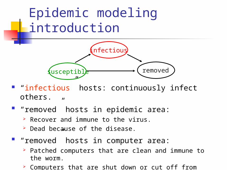
Epidemic modeling introduction
“infectious” hosts: continuously infect others. “removed” hosts in epidemic area:
Recover and immune to the virus. Dead because of the disease.
“removed” hosts in computer area: Patched computers that are clean and immune to the
worm. Computers that are shut down or cut off from worm’s
circulation.
susceptible
infectious
removed

Epidemic modeling introduction
Homogeneous assumption: Any host has the equal probability to contact any other hosts in the system. Number of contacts I S
Code Red propagation has homogeneous property: Direct connect via IP Uniformly IP scanInfectious
ISusceptible
Scontact
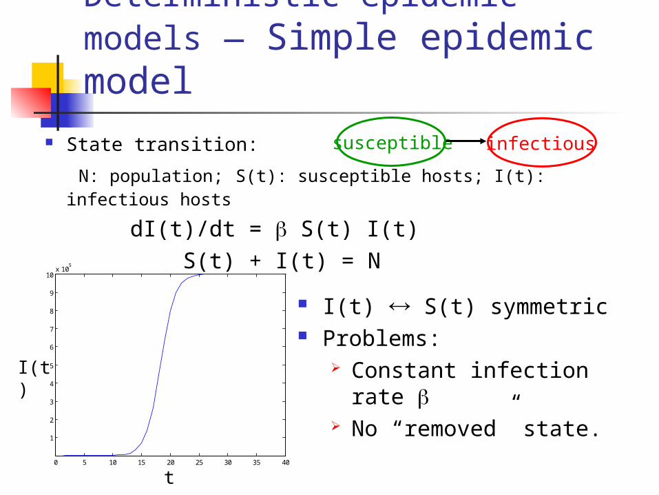
Deterministic epidemic models — Simple epidemic model
State transition:
N: population; S(t): susceptible hosts; I(t): infectious hosts
dI(t)/dt = S(t) I(t) S(t) + I(t) = N
I(t) S(t) symmetric Problems:
Constant infection rate
No “removed” state.
susceptible infectious
0 5 10 15 20 25 30 35 40
1
2
3
4
5
6
7
8
9
10x 10
5
t
I(t)
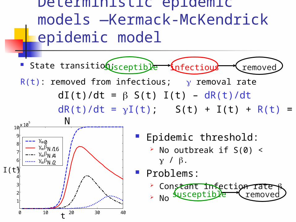
Deterministic epidemic models —Kermack-McKendrick epidemic model
State transition:
R(t): removed from infectious; removal rate
dI(t)/dt = S(t) I(t) – dR(t)/dtdR(t)/dt = I(t); S(t) + I(t) + R(t) = N
Epidemic threshold: No outbreak if S(0) < / .
Problems: Constant infection rate No
susceptible infectious removed
0 10 20 30 40
1
2
3
4
5
6
7
8
9
10x 10
5
=0=N/16=N/4=N/2
I(t)
t
susceptible removed
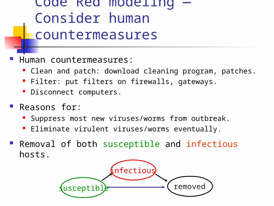
Code Red modeling — Consider human countermeasures
Human countermeasures: Clean and patch: download cleaning program, patches. Filter: put filters on firewalls, gateways. Disconnect computers.
Reasons for: Suppress most new viruses/worms from outbreak. Eliminate virulent viruses/worms eventually.
Removal of both susceptible and infectious hosts.
susceptible
infectious
removed

Code Red modeling — Consider human countermeasures
Model (extended from KM model): Q(t): removal from susceptible hosts. R(t): removal from infectious hosts. I(t): infectious hosts. J(t) I(t)+R(t): Number of infected hosts
hosts that have ever been infected
dS(t)/dt = - S(t) I(t) - dQ(t)/dtdR(t)/dt = I(t)dQ(t)/dt = S(t)J(t) S(t) + I(t) + R(t) + Q(t) = N
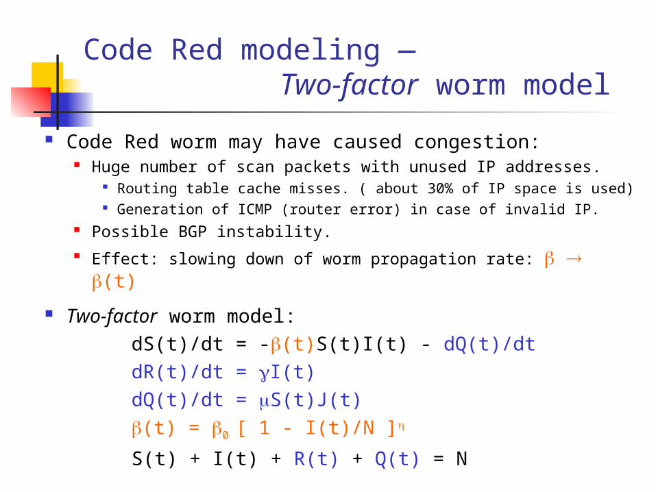
Code Red modeling — Two-factor worm model
Code Red worm may have caused congestion: Huge number of scan packets with unused IP addresses.
Routing table cache misses. ( about 30% of IP space is used) Generation of ICMP (router error) in case of invalid IP.
Possible BGP instability. Effect: slowing down of worm propagation rate: (t)
Two-factor worm model:
dS(t)/dt = -(t)S(t)I(t) - dQ(t)/dtdR(t)/dt = I(t) dQ(t)/dt = S(t)J(t) (t) = 0 [ 1 - I(t)/N ]
S(t) + I(t) + R(t) + Q(t) = N

Validation of observed data on Code Red
Network monitor: record Code Red scan traffic into the local
network. Code Red worm uniformly picked IP to scan.
# of scans a cite received Size of the IP space of the cite. # of scans a cite received at time t Overall scans in
Internet at t. # of infectious hosts sent scans to a cite at time t Overall
infectious hosts in Internet at t.
B
A
Internet
Local observation preserves global worm propagation pattern.

Observed data on Code Red worm
Two independent Class B networks: x.x.0.0/16 (1/65536 of IP space)
Count # of Code Red scan packets and source IPs for each hour.
Corresponding to infectious hosts I(t) at each hour, not infected hosts J(t)=I(t)+R(t).
Uniformly scan IP Two networks, same results.
04:00 09:00 14:00 19:00 00:00 04:000
1
2
3
4
5
6x 10
5
Dave GoldsmithKen Eichman
# scan
UTC hours (July 19-20)04:00 09:00 14:00 19:00 00:00 04:00
0
2
4
6
8
10
12x 10
4
Dave GoldsmithKen Eichman
# IP
UTC hours (July 19-20)

Code Red worm modeling — Simple epidemic
modeling
Staniford et al. used simple epidemic model approach. Conclusion from this model:
At around 20:00UTC (16:00 EDT), Code Red infected almost all susceptible hosts.
On average, a worm infected 1.8 susceptible hosts per hour.
04:00 09:00 14:00 19:00 00:00 04:000
1
2
3
4
5
6x 10
5
Dave GoldsmithKen Eichman
# scan
UTC hours (July 19-20)
0
100000
200000
300000
400000
500000
600000
2 4 6 8 10 12 14 16 18
# of Scans( Eichman)
Model
EDT hours (July 19)

Code Red worm modeling — Simple epidemic
modeling
Possible overestimation?
Issues on using simple epidemic for Code Red: Constant infection rate — No considering of the
impact of worm traffic No recovery — removal from infectious hosts No patching before infection — removal from
susceptible hosts

Code Red modeling numerical analysis —
Two-factor model
Two-factor model
12:00 14:00 16:00 18:00 20:00 22:00 24:000
2
4
6
8
10
12x 10
4
UTC hours (July 19 - 20)
I(t)
Observed DataTwo-factor model
Conclusions: At 20:00UTC (16:00 EDT), 60% ~ 70% have ever
been infected. Simple epidemic model overestimates worm spreading.
= 0.14: 14% infectious hosts would be removed after an hour.
2 4 6 8 10 12 14 16 18 200
2
4
6
8
10x 10
5
Hours
Num
ber
Infected hosts: J(t)Infectious hosts: I(t)Removal vulnerable: Q(t)

Code Red Modeling — If no congestion is
considered
If no congestion considered
12:00 14:00 16:00 18:00 20:00 22:00 24:000
2
4
6
8
10
12x 10
4
UTC hours (July 19 - 20)
I(t)
Observed DataTwo-factor model
2 4 6 8 10 12 14 16 18 200
2
4
6
8
10x 10
5
Hours
Num
ber
I(t)+R(t) I(t) Q(t)
The congestion assumption is reasonable.

Summary
We must consider the changing environment when we model virus/worm propagation. Human countermeasures/changing of behaviors. Virus/worm impact on Internet infrastructure.
Worm modeling limitation: Modeling worm continuously spreading part. Homogeneous systems.
Future work: how to predict before worm’s outbreak? Determine parameters of a virus/worm model.


