Page 1
Collaborative Adaptation of Cognitive Radio Parameters Using
Ontology and Policy Based Approach
A Dissertation Presented
by
Shujun Li
to
The Department of Electrical and Computer Engineering
in partial fulfillment of the requirements
for the degree of
Doctor of Philosophy
in the field of
Computer Engineering
Northeastern University
Boston, Massachusetts
August, 2011
Page 2
c© Copyright 2011 by Shujun Li
All Rights Reserved
i
Page 3
NORTHEASTERN UNIVERSITY
Graduate School of Engineering
Dissertation Title: Collaborative Adaptation of Cognitive Radio Parameters Using On-
tology and Policy Based Approach
Author: Shujun Li
Department: Electrical and Computer Engineering
Approved for Dissertation Requirement for the Doctor of Philosophy Degree
Dissertation Adviser: Prof. Mieczyslaw Kokar Date
Dissertation Reader: Prof. Kenneth P. Baclawski Date
Dissertation Reader: Prof. Kaushik R. Chowdhury Date
Department Chair: Ali Abur Date
ii
Page 4
Graduate School Notified of Acceptance:
Associate Dean and Director: Sara Wadia-Fascetti Date
iii
Page 5
Abstract
Cognitive radio technology has attracted an increasing interest in academic and industrial
communities. One of the motivations of cognitive radio is to enable opportunistic spec-
trum access through sensing the environment, detecting the underutilized spectrum at a
specific time and location, and adjusting the radio’s transmission parameters to conform
to spectrum utilization regulations and policies. In general, cognitive radio is expected to
have the capabilities to (1) sense the environment and collect information of the environ-
ment; (2) be aware of the external situation, the internal state and its own capabilities;
(3) automatically adapt its parameters and optimize multiple objectives; (4) reason about
communications situations, objectives and radio configurations. Some of these capabili-
ties, such as spectrum sensing and opportunistic utilization, are currently actively pursued
by various wireless research projects. The conceptual architecture that incorporates the
capabilities of awareness, reasoning and adaptation has been previously considered under
the name of Ontology Based Radio (OBR). This thesis presents a continuation of this
line of research. In particular, this dissertation focuses on using a combined approach of
ontology and policy-based control to enable collaborative adaptation of cognitive radio
parameters and thus improving the link performance. First, we developed a cognitive
radio ontology that covers the basic terms of wireless communications from the PHY and
MAC layers. Second, we selected a use case of collaborative link adaptation. Third, we
developed a set of policies that are needed for this use case. The whole framework was
implemented on the USRP/GNU Radio platform. The validity, cost and benefits of the
ontology and policy based approach to collaborative radio control was assessed using both
Matlab simulations and the implementation on the GNU radio platform.
Page 6
Contents
Abstract i
List of Tables v
List of Figures vii
1 Introduction 1
1.1 Foundation of Cognitive Radio: Software-Defined Radio . . . . . . . . . . 2
1.2 Definition of Cognitive Radio . . . . . . . . . . . . . . . . . . . . . . . . . 5
1.3 Expected Capabilities of Cognitive Radio . . . . . . . . . . . . . . . . . . 6
1.3.1 Sensing . . . . . . . . . . . . . . . . . . . . . . . . . . . . . . . . . 6
1.3.2 Awareness and Reasoning . . . . . . . . . . . . . . . . . . . . . . . 7
1.3.3 Automatic Adaptation/Optimization . . . . . . . . . . . . . . . . . 8
1.4 Architecture of Cognitive Radio . . . . . . . . . . . . . . . . . . . . . . . . 9
1.5 Cognitive Radio Agent . . . . . . . . . . . . . . . . . . . . . . . . . . . . . 13
1.5.1 Knobs and Meters . . . . . . . . . . . . . . . . . . . . . . . . . . . 14
1.5.2 Control Model . . . . . . . . . . . . . . . . . . . . . . . . . . . . . 19
1.6 Dissertation Organization . . . . . . . . . . . . . . . . . . . . . . . . . . . 20
2 Link Adaptation: Problem Formulation 21
2.1 Description of Communications Parameters . . . . . . . . . . . . . . . . . 21
i
Page 7
2.1.1 Channel Parameters . . . . . . . . . . . . . . . . . . . . . . . . . . 22
2.1.2 Transmitter Parameters . . . . . . . . . . . . . . . . . . . . . . . . 23
2.1.3 Receiver Parameters . . . . . . . . . . . . . . . . . . . . . . . . . . 24
2.1.4 Parameters Summary . . . . . . . . . . . . . . . . . . . . . . . . . 25
2.2 Objective Function . . . . . . . . . . . . . . . . . . . . . . . . . . . . . . . 27
2.3 Constraints . . . . . . . . . . . . . . . . . . . . . . . . . . . . . . . . . . . 28
2.4 Formal Description of Link Adaptation Process . . . . . . . . . . . . . . . 32
3 Literature Review 34
3.1 Exhaustive Search . . . . . . . . . . . . . . . . . . . . . . . . . . . . . . . 34
3.2 Genetic Algorithms . . . . . . . . . . . . . . . . . . . . . . . . . . . . . . . 35
3.3 Case-based Reasoning . . . . . . . . . . . . . . . . . . . . . . . . . . . . . 36
3.4 Game Theory . . . . . . . . . . . . . . . . . . . . . . . . . . . . . . . . . . 37
3.5 Expert Systems . . . . . . . . . . . . . . . . . . . . . . . . . . . . . . . . . 38
3.6 Ontology Based Radio . . . . . . . . . . . . . . . . . . . . . . . . . . . . . 39
4 Design Options and Proposed Solution 41
4.1 Knowledge-less vs. Knowledge-based Approaches . . . . . . . . . . . . . . 41
4.2 Language Selection for Ontology-Based Radio . . . . . . . . . . . . . . . 44
4.2.1 Imperative Language vs. Declarative Language . . . . . . . . . . . 47
4.2.2 Ontology Language . . . . . . . . . . . . . . . . . . . . . . . . . . 50
4.2.3 Policy Language . . . . . . . . . . . . . . . . . . . . . . . . . . . . 52
4.3 Non-Collaborative Adaptation vs. Collaborative Adaptation . . . . . . . 54
4.4 Fixed Protocol vs. Flexible Signaling . . . . . . . . . . . . . . . . . . . . . 57
4.5 Summary of the Proposed Solution . . . . . . . . . . . . . . . . . . . . . . 58
5 Cognitive Radio Ontology 61
5.1 Overview . . . . . . . . . . . . . . . . . . . . . . . . . . . . . . . . . . . . 61
5.2 Principles of Modeling . . . . . . . . . . . . . . . . . . . . . . . . . . . . . 62
ii
Page 8
5.2.1 Top-Level Classes . . . . . . . . . . . . . . . . . . . . . . . . . . . 62
5.2.2 Further Distinction: Object and Process . . . . . . . . . . . . . . . 65
5.2.3 Part-Whole Relationship . . . . . . . . . . . . . . . . . . . . . . . . 68
5.2.4 Attribute, Properties, Parameters and Arguments . . . . . . . . . 73
5.3 Object . . . . . . . . . . . . . . . . . . . . . . . . . . . . . . . . . . . . . . 76
5.3.1 Alphabet and AlphabetTableEntry . . . . . . . . . . . . . . . . . . 76
5.3.2 Channel . . . . . . . . . . . . . . . . . . . . . . . . . . . . . . . . . 76
5.3.3 ChannelModel . . . . . . . . . . . . . . . . . . . . . . . . . . . . . 78
5.3.4 Packet and Packet Field . . . . . . . . . . . . . . . . . . . . . . . . 79
5.3.5 Signal . . . . . . . . . . . . . . . . . . . . . . . . . . . . . . . . . . 81
5.3.6 Burst . . . . . . . . . . . . . . . . . . . . . . . . . . . . . . . . . . 85
5.3.7 Sample . . . . . . . . . . . . . . . . . . . . . . . . . . . . . . . . . 86
5.3.8 Symbol . . . . . . . . . . . . . . . . . . . . . . . . . . . . . . . . . 87
5.3.9 PNCode . . . . . . . . . . . . . . . . . . . . . . . . . . . . . . . . . 89
5.3.10 Component . . . . . . . . . . . . . . . . . . . . . . . . . . . . . . . 90
5.3.11 TransceiverPreset, Transfer Functions and Constraints of Transfer
Functions . . . . . . . . . . . . . . . . . . . . . . . . . . . . . . . . 104
5.3.12 Detector and DetectionEvidence . . . . . . . . . . . . . . . . . . . 108
5.3.13 Network, Network Membership and Role . . . . . . . . . . . . . . . 110
5.3.14 Agent and Goal . . . . . . . . . . . . . . . . . . . . . . . . . . . . . 111
5.4 Process . . . . . . . . . . . . . . . . . . . . . . . . . . . . . . . . . . . . . 113
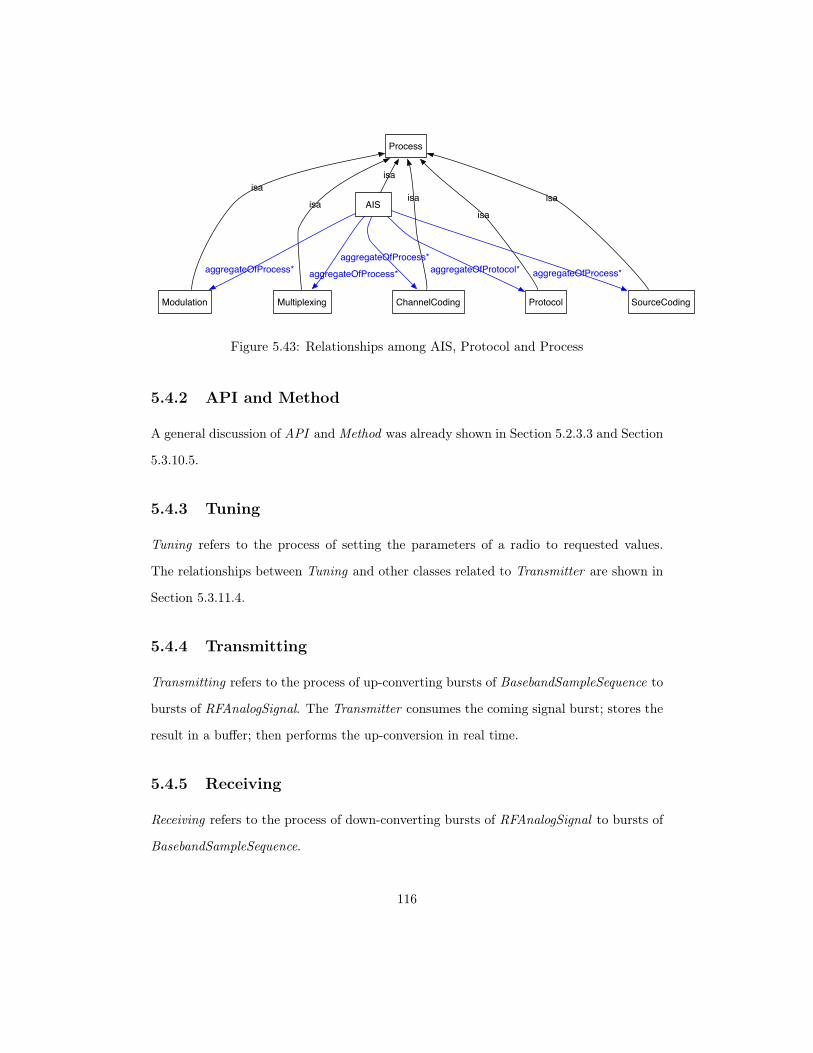
5.4.1 AIS and Protocol . . . . . . . . . . . . . . . . . . . . . . . . . . . . 113
5.4.2 API and Method . . . . . . . . . . . . . . . . . . . . . . . . . . . . 116
5.4.3 Tuning . . . . . . . . . . . . . . . . . . . . . . . . . . . . . . . . . . 116
5.4.4 Transmitting . . . . . . . . . . . . . . . . . . . . . . . . . . . . . . 116
5.4.5 Receiving . . . . . . . . . . . . . . . . . . . . . . . . . . . . . . . . 116
5.4.6 SourceCoding . . . . . . . . . . . . . . . . . . . . . . . . . . . . . . 117
5.4.7 ChannelCoding . . . . . . . . . . . . . . . . . . . . . . . . . . . . . 117
iii
Page 9
5.4.8 Modulation . . . . . . . . . . . . . . . . . . . . . . . . . . . . . . . 117
5.4.9 Multiplexing . . . . . . . . . . . . . . . . . . . . . . . . . . . . . . 117
5.4.10 PNSequenceGeneration . . . . . . . . . . . . . . . . . . . . . . . . 117
5.4.11 BehaviorModel . . . . . . . . . . . . . . . . . . . . . . . . . . . . . 117
5.5 Value . . . . . . . . . . . . . . . . . . . . . . . . . . . . . . . . . . . . . . 121
5.6 Quantity and UnitOfMeasure . . . . . . . . . . . . . . . . . . . . . . . . . 123
5.7 Summary and Future Work . . . . . . . . . . . . . . . . . . . . . . . . . . 124
6 Policy-based Radio Control 125
6.1 Policies for Link Establishment . . . . . . . . . . . . . . . . . . . . . . . . 127
6.2 Policies for Link Adaptation . . . . . . . . . . . . . . . . . . . . . . . . . . 130
7 Simulation in MATLAB 132
8 Implementation on GNU/USRP 134
8.1 Implementation Architecture . . . . . . . . . . . . . . . . . . . . . . . . . 134
8.2 Message Structure . . . . . . . . . . . . . . . . . . . . . . . . . . . . . . . 136
8.3 State Machine . . . . . . . . . . . . . . . . . . . . . . . . . . . . . . . . . . 139
8.4 Policy Execution Results . . . . . . . . . . . . . . . . . . . . . . . . . . . . 143
9 Evaluation 145
9.1 Performance Improvement . . . . . . . . . . . . . . . . . . . . . . . . . . . 146
9.2 Processing Delay . . . . . . . . . . . . . . . . . . . . . . . . . . . . . . . . 149
9.3 Control Message Overhead . . . . . . . . . . . . . . . . . . . . . . . . . . . 151
9.4 Inference Capability . . . . . . . . . . . . . . . . . . . . . . . . . . . . . . 153
9.5 Flexibility . . . . . . . . . . . . . . . . . . . . . . . . . . . . . . . . . . . . 157
10 Summary 164
iv
Page 10
List of Tables
2.1 Parameters Summary . . . . . . . . . . . . . . . . . . . . . . . . . . . . . 26
2.2 Constraints of the Link Adaptation Problem . . . . . . . . . . . . . . . . . 33
4.1 Imperative Language vs. Declarative Language (1) . . . . . . . . . . . . . 48
4.2 The Description of the Percepts, Actions, Goals and Environment for the
Radio Agent in the Link adaptation Problem . . . . . . . . . . . . . . . . 56
5.1 Examples of Objects and Process . . . . . . . . . . . . . . . . . . . . . . . 65
5.2 Example of Alphabet Table . . . . . . . . . . . . . . . . . . . . . . . . . . 76
5.3 Properties of PacketField . . . . . . . . . . . . . . . . . . . . . . . . . . . 81
5.4 Properties of Signal . . . . . . . . . . . . . . . . . . . . . . . . . . . . . . . 84
5.5 Properties of Burst . . . . . . . . . . . . . . . . . . . . . . . . . . . . . . . 86
5.6 Subclasses of Component . . . . . . . . . . . . . . . . . . . . . . . . . . . 91
5.7 Transmitter API (1): TransmitControl . . . . . . . . . . . . . . . . . . . . 102
5.8 Transmit API (2): TransmitDataPush . . . . . . . . . . . . . . . . . . . . 102
5.9 Properties of ChannelMask, SpectrumMask and GroupDelayMask . . . . 106
5.10 Properties of Transmitter . . . . . . . . . . . . . . . . . . . . . . . . . . . 108
5.11 Properties of Detector and its Subclasses . . . . . . . . . . . . . . . . . . . 109
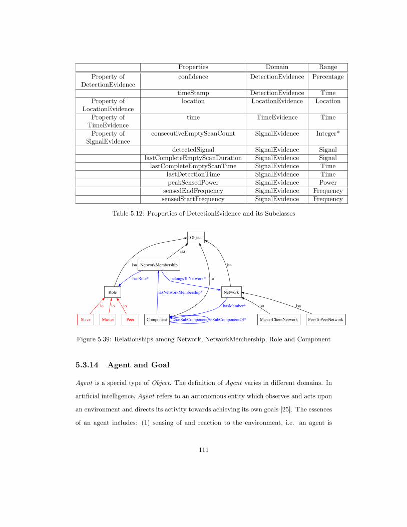
5.12 Properties of DetectionEvidence and its Subclasses . . . . . . . . . . . . . 111
5.13 Properties of Value . . . . . . . . . . . . . . . . . . . . . . . . . . . . . . . 123
5.14 Overview of Quantity and UnitOfMeasure . . . . . . . . . . . . . . . . . . 124
v
Page 11
8.1 Types of Control Message . . . . . . . . . . . . . . . . . . . . . . . . . . . 137
9.1 Flexibility Comparison . . . . . . . . . . . . . . . . . . . . . . . . . . . . 160
9.2 Expressiveness Comparison . . . . . . . . . . . . . . . . . . . . . . . . . . 162
vi
Page 12
List of Figures
1.1 Architecture of Cognitive Radio . . . . . . . . . . . . . . . . . . . . . . . . 11
1.2 Agent Interacts with the Environment . . . . . . . . . . . . . . . . . . . . 14
1.3 Architecture of Two Cognitive Radios . . . . . . . . . . . . . . . . . . . . 19
1.4 Example of Cognitive Radio Control Model . . . . . . . . . . . . . . . . . 20
4.1 Actors, issues and standard languages: a conceptual view (Source: [66]) . 46
4.2 Imperative Language vs. Declarative Language (2) . . . . . . . . . . . . . 50
4.3 Sequence Diagram of Collaborative Link Adaptation . . . . . . . . . . . . 56
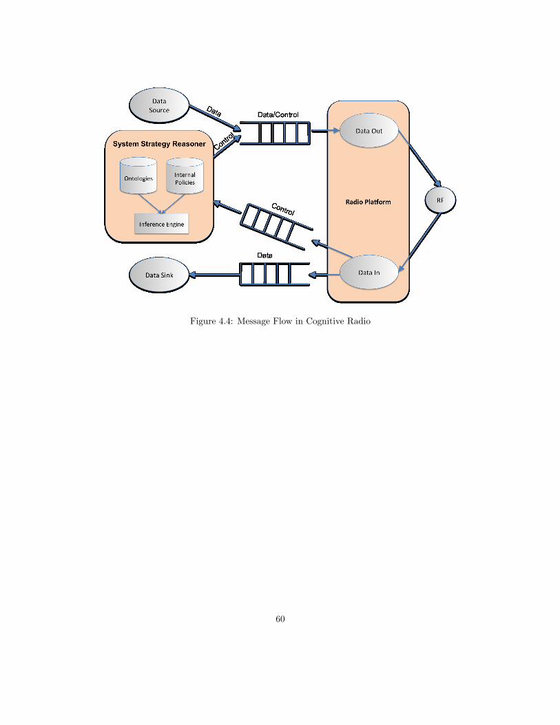
4.4 Message Flow in Cognitive Radio . . . . . . . . . . . . . . . . . . . . . . . 60
5.1 Top-Level Classes of CRO . . . . . . . . . . . . . . . . . . . . . . . . . . . 63
5.2 Naming Schemes for Aggregation and Composition . . . . . . . . . . . . . 69
5.3 Packet Frame Structure . . . . . . . . . . . . . . . . . . . . . . . . . . . . 70
5.4 Example of Part-Whole Relationship (1): Alphabet and AlphabetTableEntry 70
5.5 Example of Part-Whole Relationship (2): API and Method . . . . . . . . 71
5.6 Example of Part-Whole Relationship (3): Radio and RadioComponent . . 72
5.7 Example of Part-Whole Relationship (4): Signal . . . . . . . . . . . . . . 73
5.8 Representation of Properties and Attributes: Example of Transceiver . . . 75
5.9 Subclasses of Channel . . . . . . . . . . . . . . . . . . . . . . . . . . . . . 77
5.10 Relationships among Channel, ChannelModel, Multiplexing and Modulation 78
5.11 Subclasses of Channel Model . . . . . . . . . . . . . . . . . . . . . . . . . 79
vii
Page 13
5.12 Relationships among Packet, Packefield and Protocol . . . . . . . . . . . . 80
5.13 Subclasses of Packet Class . . . . . . . . . . . . . . . . . . . . . . . . . . . 80
5.14 subclasses of PacketField . . . . . . . . . . . . . . . . . . . . . . . . . . . . 81
5.15 Signal Processing in SDR . . . . . . . . . . . . . . . . . . . . . . . . . . . 82
5.16 Subclasses of Signal Class . . . . . . . . . . . . . . . . . . . . . . . . . . . 84
5.17 Illustration of BasebandBurst and RFBurst (Source: [54]) . . . . . . . . . 85
5.18 Relationships among Burst, Signal and Packet . . . . . . . . . . . . . . . . 86
5.19 Properties of Sample . . . . . . . . . . . . . . . . . . . . . . . . . . . . . . 87
5.20 Properties of Symbol . . . . . . . . . . . . . . . . . . . . . . . . . . . . . . 88
5.21 Illustration of InformationBitsPerSymbol (Source: [56, 50]) . . . . . . . . 88
5.22 Relationships among Signal, Sample and Symbol . . . . . . . . . . . . . . 89
5.23 Subclasses of PNCode . . . . . . . . . . . . . . . . . . . . . . . . . . . . . 89
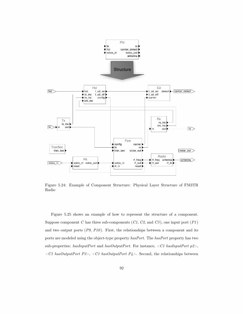
5.24 Example of Component Structure: Physical Layer Structure of FM3TR
Radio . . . . . . . . . . . . . . . . . . . . . . . . . . . . . . . . . . . . . . 92
5.25 Representation of Component Structure . . . . . . . . . . . . . . . . . . . 93
5.26 Relationships between Component and Port . . . . . . . . . . . . . . . . . 93
5.27 Top-Level Component Structure of FM3TR Radio . . . . . . . . . . . . . 95
5.28 OWL Representation of FM3TR Radio . . . . . . . . . . . . . . . . . . . . 96
5.29 Structures and Behavior Model of FM3TR Physical Layer Component . . 98
5.30 Relationships between Component and BehaviorModel . . . . . . . . . . . 99
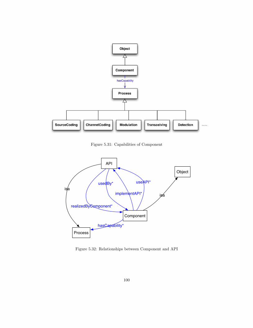
5.31 Capabilities of Component . . . . . . . . . . . . . . . . . . . . . . . . . . . 100
5.32 Relationships between Component and API . . . . . . . . . . . . . . . . . 100
5.33 Overview of Transmitter API . . . . . . . . . . . . . . . . . . . . . . . . . 101
5.34 OWL Representation of Transmitter API . . . . . . . . . . . . . . . . . . 103
5.35 Characteristics of Spectrum Mask (Source: [54]) . . . . . . . . . . . . . . 105
5.36 Characteristics of GroupDelayMask (Source: [54]) . . . . . . . . . . . . . 105
5.37 Characteristics of Transceiver . . . . . . . . . . . . . . . . . . . . . . . . . 107
5.38 Relationships between Detector and DetectionEvidence . . . . . . . . . . 110
viii
Page 14
5.39 Relationships among Network, NetworkMembership, Role and Component 111
5.40 Relationships between Agent and Goal . . . . . . . . . . . . . . . . . . . . 113
5.41 Air Interface Layering Architecture (Source: [24]) . . . . . . . . . . . . . . 114
5.42 Default Protocols of cdma2000 1xEV-DO (Source: [24] . . . . . . . . . . . 115
5.43 Relationships among AIS, Protocol and Process . . . . . . . . . . . . . . . 116
5.44 Subclasses of BehaviorModel . . . . . . . . . . . . . . . . . . . . . . . . . 118
5.45 State Transition Table . . . . . . . . . . . . . . . . . . . . . . . . . . . . . 119
5.46 OWL Representation of State Transition Diagram . . . . . . . . . . . . . 120
5.47 Physical Layer FSM Specification of a FM3TR Radio . . . . . . . . . . . 121
5.48 OWL Representation of the Physical Layer FSM of FM3TR Radio . . . . 122
6.1 Example Rule in BaseVISor Format . . . . . . . . . . . . . . . . . . . . . 126
6.2 Example of Procedural Attachment . . . . . . . . . . . . . . . . . . . . . . 127
6.3 Illustration of Policy-based Radio Control . . . . . . . . . . . . . . . . . . 128
6.4 Sequence Diagram of Link Adaptation (1) : Query and Request . . . . . . 129
7.1 MATLAB Simulation Results: Comparison of Policy 1, Policy 2, Policy 3 133
8.1 Implementation Architecture . . . . . . . . . . . . . . . . . . . . . . . . . 135
8.2 Example of Request Message . . . . . . . . . . . . . . . . . . . . . . . . . 138
8.3 Example of Agree Message . . . . . . . . . . . . . . . . . . . . . . . . . . . 138
8.4 Sequence Diagram of Link Adaptation (2): Call-For-Proposal . . . . . . . 140
8.5 Finite-State-Machine of Call-For-Proposal . . . . . . . . . . . . . . . . . . 141
8.6 Finite-State-Machine of Query . . . . . . . . . . . . . . . . . . . . . . . . 142
8.7 Finite-State-Machine of Request . . . . . . . . . . . . . . . . . . . . . . . 142
8.8 Policy Execution Results . . . . . . . . . . . . . . . . . . . . . . . . . . . . 144
9.1 Performance Evaluation (1): Mean Signal-to-Noise-Ratio . . . . . . . . . . 147
9.2 Performance Evaluation (2): Power Efficiency . . . . . . . . . . . . . . . . 147
9.3 Performance Evaluation (3): Corrupted Packet Rate . . . . . . . . . . . . 148
ix
Page 15
9.4 Performance Evaluation (4): Overall Performance . . . . . . . . . . . . . . 149
9.5 Response Time of Each Control Message . . . . . . . . . . . . . . . . . . . 150
9.6 Control Message Overhead . . . . . . . . . . . . . . . . . . . . . . . . . . . 152
9.7 Extend CRO with Configuration Class . . . . . . . . . . . . . . . . . . . . 153
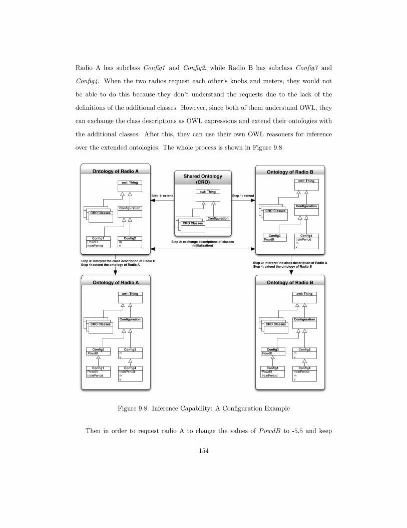
9.8 Inference Capability: A Configuration Example . . . . . . . . . . . . . . . 154
9.9 Instance of Config3 . . . . . . . . . . . . . . . . . . . . . . . . . . . . . . . 155
9.10 Inference Capability of OWL Ontology . . . . . . . . . . . . . . . . . . . . 156
9.11 Implementation of Control Information . . . . . . . . . . . . . . . . . . . . 159
9.12 Examples of Control Messages Between Radios . . . . . . . . . . . . . . . 163
x
Page 16
Chapter 1
Introduction
In recent years, cognitive radio technology has attracted an increasing interest in aca-
demic and industrial communities. One of the motivating factors for introducing cog-
nitive radio comes from the underutilization of radio spectrum. Evidence shows that
on average, less than 5%, and possibly as little as 1%, of the spectrum below 3GHz, as
measured in frequency-space-time, is used [4]. There is spectrum that is never accessed
or accessed only for a fraction of time. Since radio spectrum is a precious and expen-
sive resource ($200M/MHz in the most recent US auction), a more efficient utilization of
free spectrum, also called the “white spaces”, is of huge economic value. Cognitive radio
technology enables opportunistic spectrum access that senses the environment, detects
the underutilized spectrum at a specific time and location, and then adjusts the radio’s
transmission parameters to conform to the opportunity without harmful degradation to
the primary user [4].
From the user’s perspective, the essential desirable capabilities of cognitive radio could
include the following aspects [4]:
• Spectrum management and optimization. Currently, the allocation and uti-
lization of spectrum follows a “command and control” structure which is dominated
by long planning cycles, exclusivity assumptions, conservative worst case analysis
1
Page 17
and litigious regulatory proceedings. Using spectrum-aware radios, the management
of spectrum could be transitioned into a new structure that is embedded within each
individual radio. Collectively, implicitly or explicitly, the radios would cooperate to
optimize the allocation of the spectrum to meet RF devices’ needs.
• Intelligent interaction with the network. Cognitive radio could provide stan-
dardized interfaces to access heterogeneous networks and support the management
and optimization of network resources.
• Intelligent interaction with the user. Cognitive radio could support vision
and speech perception. For example, it could use vision algorithms, machine learn-
ing techniques, reinforcement learning and case-based reasoning to understand the
world around the user and detect opportunities to assist the user using this infor-
mation. Also, it could use speech recognition technology to perceive conversations,
retrieve and analyze the content of conversations.
1.1 Foundation of Cognitive Radio: Software-Defined
Radio
Cognitive radio is most efficiently built on Software-Defined Radio (SDR). The definition
of SDR is given by IEEE SCC41-P1900.1 as the “radio in which some or all the physical
layer functions are software defined”. The properties defined by software include carrier
frequency, signal bandwidth, modulation, network access, cryptography, channel coding
(e.g. forward error correction coding) and source coding (voice, video and data). SDR is
a general-purpose device with the platform that can adapt to a wide range of waveforms,
applications and products. Different kinds of waveforms at different frequencies can be
implemented on the same SDR processor. Thus SDR is cost effective, versatile and easy
to upgrade (reduced development cycle time).
Typically, an SDR is decomposed into a stack of hardware and software functions,
2
Page 18
each with open standard interfaces. The SDR hardware architecture usually consists of
the RF Front End, A/D converter, and the Digital Back End. First, the RF Front End
amplifies the received signal, and then converts the carrier frequency of the signal to a
low intermediate frequency. Second, the A/D converter converts the analog signal to a
digital signal proportional to the magnitude of the analog signal. Third, the digital signal
is further processed by a digital signal processor (in the Digital Back End) to perform the
modem (modulation-demodulation) functions [4].
The RF Front End usually consists of receiver and transmitter analog functions such
as frequency up-converters and down-converters, filters, and amplifiers. In the full-duplex
mode, there will be some filtering to keep the high-power transmitted signal from inter-
fering with the low-power received signal [4].
The Digital Back End consists of General-Purpose Processors (GPP), Field-Programmable
Gate Arrays (FPGAs) and Digital Signal Processors (DSP). A GPP usually performs the
user applications and high-level communications protocols, whereas a DSP is more effi-
cient in terms of signal processing but less capable to process high-level communications
protocols. For example, speech and video applications usually run on a DSP, whereas
text and web browsing typically run on a GPP. On the other hand, an FPGA comple-
ments DSPs in that it provides timing logic to synthesize clocks, baud rate, chip rate,
time slot and frame timing, resulting in a more compact waveform implementation. In
general, the SDR hardware design is a mixture of GPPs, FPGAs and DSPs to provide
flexible platform to implement various waveforms and applications. Dedicated-purpose
Application-Specific Integrated Circuits (ASIC) are not suitable for SDR hardware due
to their lack of flexibility [4].
The Digital Back End is used to implement functions such as modem, Forward Error
Correction (FEC), Medium Access Control (MAC) and user applications. The modem
converts symbols to bits by a sequence of operations. First, the digital down-converter
(DDC) converts the digitized real signal centered at an intermediate frequency to a base-
band complex signal at a lower sampling rate. Second, the signal is filtered to the desired
3
Page 19
bandwidth. Next, the signal is time-aligned, despreaded and re-filtered. Then, a symbol
detector is used to time-align signal to symbols. An equalizer is also used to correct for
channel multipath effect and filter delay distortions. Finally, the symbol is mapped to
bits using the modulation alphabet. Due to interference, the signal may be received with
errors. FEC uses the redundancy introduced in the channel coding process to detect and
correct the errors. FEC can be integrated with the demodulator or the MAC processing.
After the MAC layer processing and network layer processing, the data is passed to the
application layer that performs user functions and interfaces such as speaker/microphone,
GUI, and other human-computer interfaces. The user application layer usually includes
vocoder, video coder, data coder and web browser functions. Typically, voice applica-
tions are implemented in DSP or GPP. Video applications are usually implemented on
special-purpose processors due to the extensive cross-correlation required to calculate the
motion vectors of the video image objects. Text and web browsing usually run on GPP
[4].
On top of the hardware, several layers of software are installed, including the operating
system, boot loader, board support package and the Hardware Abstraction Layer (HAL).
It is essential to present a set of highly standardized interfaces between the hardware
platform and the software, and between the software modules so that the waveform and
applications can be installed, used and replaced flexibly to achieve the user’s goals [4].
There are two open SDR architectures – Software Communication Architecture (SCA)
and GNU radio [6]. SCA is a standardized software architecture sponsored by the Joint
Program Office (JPO) of the US Department of Defense (DoD) for secure signal-processing
applications on heterogeneous, distributed hardware. It is a core framework to provide the
infrastructure to create, install and manage various waveforms, as well as to control and
manage the hardware. In addition, it provides a set of standardized interfaces to enable
the interaction with external services. GNU radio is a Python-based architecture that
provides a collection of signal processing components to build and deploy SDR systems.
It is designed to run on general-purpose computers on the Linux operating system [4].
4
Page 20
1.2 Definition of Cognitive Radio
Cognitive radio (CR) is a collection of applications that are built on top of SDR. In order
to evolve SDR to cognitive radio, many technologies must converge to enable cognitive
radio to adapt for the spectrum regulator, the network operator and the user objectives.
The definition of cognitive radio was first introduced by Mitola in the late 1990’s [2],
and then refined to the following (as reported in [34]):
“A really smart radio that would be self, RF- and User-aware, and that
would include language technology and machine vision along with a lot of
high-fidelity knowledge of the radio environment.”
Since then, the definition of cognitive radio has been offered by a number of industry
leaders, academia and others. Here are some of the CR definitions [16]:
Intel Corporation (in early 2004):
“Radios that automatically find and access unused spectrum across different
networks (licensed and un-licensed including the features of optimization and
adaption) [36].
Optimization: Find the best link (in space, time) based on user require-
ments, e.g., cost per unit throughput, latency.
Continuously Adapt: Seamlessly roam across the networks always main-
taining the ‘best link’ possible” [35].
ITU Radio Communication Study Group:
“A radio or system that senses, and is aware of, its operational environment
and can dynamically and autonomously adjust its radio operating parameters
accordingly.” [37]
5
Page 21
Dr. Simon Haykin (Professor of McMaster University) [38]:
“Cognitive radio is an intelligent wireless communication system that is
aware of its surrounding environment (i.e., outside world), and uses the method-
ology of understanding-by-building to learn from the environment and adapt
its internal states to statistical variations in the incoming RF stimuli by mak-
ing corresponding changes in certain operational parameters (e.g., transmit
power, carrier frequency, and modulation strategy) in real-time, with two pri-
mary objectives in mind:
• Highly reliable communications whenever and wherever needed;
• Efficient utilization of the radio spectrum.
In this thesis, we use the definition of cognitive radio given by SDR Forum [15]:
1. “Radio in which communications systems are aware of their environ-
ment and internal state, and can make decisions about their radio operating
behavior based on that information and predefined objectives. The environ-
mental information may or may not include location information related to
communication systems.
2. Radio that uses SDR, adaptive radio and other technologies to automat-
ically adjust its behavior or operations to achieve desired objectives.”
1.3 Expected Capabilities of Cognitive Radio
Based on the definition provided in [15], the Wireless Innovation Forum has identified the
capabilities that are essential to cognitive radios [16].
1.3.1 Sensing
Sensing refers to the ability to collect the information regarding its awareness of its
environment. Sensing can be locally performed and self contained in a radio or can be
6
Page 22
remotely performed elsewhere in the network. As one of the most important sensing
abilities, spectrum sensing measures the characteristics of received signals and RF energy
levels in order to determine whether a particular section of spectrum is occupied [16].
On the other hand, the radio can also sense its internal status by using, for instance,
Java reflection [29]. Java reflection provides a means to query the internal parameters,
such as the signal-to-noise ratio, frequency offset, timing offset or equalizer taps without
hard-coding. By examining these parameters, the receiver can determine what change at
the receiver can improve the performance of the communication link. Then the receiver
can negotiate with the transmitter on how to adjust these parameters in order to achieve
the goals.
1.3.2 Awareness and Reasoning
According to [16], awareness is the ability to interpret and derive understanding from the
input information. For example, the cognitive radio should be able to interpret that the
received radio frequency energy indicates how much a section of spectrum is occupied at
a point in space.
Situation Awareness and self-awareness have been identified as one of the most impor-
tant features in cognitive radio [12]. For example, the radio can collect the information
from the user and the environment and store it in its memory. However, this information
does not guarantee that the radio is aware of the situation of its user. Situation Awareness
is the awareness with respect to the surrounding environment, including the perception of
the elements in the environment, the comprehension of their meaning, and the projection
of their status in the near future [39].
In other words, the agent needs to know not only about the status of the objects of
interest, but also the relationship between themselves, as well as the future of the object
states and the relationships. Therefore, to predict the future states and derive rules for
determining the relationships, models and dynamics of the objects are required [12].
One example of the relevant relationship is that based on the source and destination
7
Page 23
information provided by the user, the radio can derive the path from the source to the
destination.
Self-awareness refers to the ability of the radio to understand its own capabilities, i.e.,
to understand what it does and does not know, as well as the limits of its capabilities.
In this way, the radio can determine whether a task is within its capabilities. In the case
of a basic self-aware radio, it should know its current performance such as bit-error rate,
signal-to-interference and noise ratio and multipath interference, etc. A more advanced
agent has the capability to reflect on its previous actions and their results, e.g., extracting
parameters from logs. Another example is that for a self-aware radio to decide whether it
should search for the specific entries in the log and then perform appropriate calculations
(or simply guess), it needs more information about the task, such as the effort required
to perform such a task and the required accuracy of the estimate [12].
As was explain above, real awareness can be achieved only if the agent can reason about
the facts it gets from the environment or from other agents. Reasoning refers to the ability
to infer implicit knowledge from the explicitly represented knowledge. Reasoning requires
(1) a proper language to represent the knowledge and policies, and (2) a reasoning engine
that can process the knowledge and rules. This issue will be discussed in more detail in
Section 4.2.
1.3.3 Automatic Adaptation/Optimization
A radio may have different levels of adaptation/optimization [7].
(1) At a low level, the adaptation algorithm is built into hardware. For instance, in
802.11a, radios are able to sense the bit error rate and then adapt the modulation to
a data rate and then forward error correction (FEC) such that the bit error rate can
be controlled at an acceptable low level. This algorithm is implemented in application-
specific integrated circuits (ASIC) chips.
(2) At an intermediate level, the adaptation is software-defined. One way to achieve it
is to hard code the adaptation algorithm into the radio. The shortcoming of this approach
8
Page 24
is that the algorithm is hard-coded into the radio and forms an inseparable part of the
radio’s firmware. Another way is to write the adaptation algorithm into a set of policies
that control the radio behavior. This approach separates the adaptation policies from the
implementation and thus exhibits more flexibility on the modification of the adaptation
algorithm.
(3) At the high level, the radio is able to learn from its experience and adapt its param-
eters without human interventions. Learning means that when the system is presented
with a set of environmental test stimuli, the decisions it arrives at are not constant, but
improve with time and experience. A typical example of learning is the case-based rea-
soning. The radio records the perception, the action and the result of each case from its
past experience. In this way, the radio will gradually learn more about the environment,
and better adapt to the environment. A critical difference between policy-based radio
and cognitive radio is that a cognitive radio has the learning capability while the policy-
based radio does not. By learning we mean that if presented with the same set of input
conditions, a policy-based radio should always arrive at the same conclusion regarding
how the radio should operate, while a cognitive radio may react differently depending on
how it perceives the environment [16].
1.4 Architecture of Cognitive Radio
The core of a cognitive radio includes endogenous components and exogenous components
[8]. An exogenous component executes and enforces external policies. It addresses the
radio’s impact on the external environment, and ensures that the behaviors of the radio
satisfy the constraints imposed by external regulations and policies. For example, an ex-
ogenous component can assist the radio in avoiding spectrum interference while searching
for spectrum opportunities. Conversely, an endogenous component internally optimizes
the performance of the radio through selection of operating mode and other parameters.
Based on the above perspective, the basic architecture of a cognitive radio that ad-
9
Page 25
dresses the distinction between endogenous and exogenous components can be viewed
[14, 17, 79] as in Figure 1.1. The abstract architecture of a cognitive radio comprises
eight components:
1. Sensors. In a cognitive radio, sensors are used to collect the information from the
external environment and discover available spectrum and transmission opportuni-
ties.
2. Radio Frequency (RF). The RF component is used to transmit and receive signal.
3. Radio Platform. The radio platform includes the digital signal processing and the
software control. It provides interfaces to communicate with the RF, sensors, infor-
mation source and sink, and the policy reasoners.
4. System Strategy Reasoner (SSR). The SSR is an endogenous component of the cog-
nitive radio. It forms strategies to control the operation of the radio. The strategies
reflects the spectral opportunities, the capabilities of the radio and waveform, and
the needs of the network and the users.
5. Policy Conformance Reasoner (PCR). The PCR is the exogenous component of the
cognitive radio. It executes the active policy set to ensure that the radio transmis-
sion conforms to the policy.
6. Policy Enforcer (PE). The PE acts as a gateway between the SSR and the Radio
Platform. It ensures that all the transmission strategy sent from SSR to the Radio
Platform complies with the active policy.
7. Global Policy Repository. The Global Policy Repository stores all the policies and
specific subsets configured for specific networks. The Global Policy Repository is
shared across the network.
8. Local Policy Repository. The Local Policy Repository is within the SSR. It can
download the policies from the Global Policy Repository through an interface. A
10
Page 26
radio node can store multiple sets of policies, but only one set of policy is active at
any time.
RF
Global Policy Repository
Policy Conformance Reasoner
Local Policy Repository
System Strategy Reasoner
Policy Enforcer
Radio Platform
Sensor
RequestOpportunities
Allow/Deny
Data Source/Sink
Figure 1.1: Architecture of Cognitive Radio
The SSR is the most important component in this architecture. The interactions
between SSR and other components are shown as follows:
SSR and PCR The SSR sends query/request to the PCR when the radio needs to
change its transmission strategy, or at the end of the validity time period for a permitted
transmission opportunity[17, 14].
In the former case, the SSR sends the following types of message to the PCR:
11
Page 27
• Unbounded transmission request. The SSR asks PCR to assist in identifying trans-
mission parameters that are policy compliant. The request may not have values
specified for all transmission parameters. For example, the SSE may ask: "I want
to send a packet to Radio_B at time_T and at place_P, which waveform should I
use?" The PCR will identify the transmission parameters that meet both the needs
of the SSR’s request and comply with the active policy set. Then, the PCR sends
a reply back to the SSE. The reply includes the transmission parameters such as
transmission power, frequency, data rate, modulation, and so on.
• Bounded transmission request. The SSR sends a fully bounded transmission request
to the PCR. The PCR evaluates the request to confirm that whether it complies
with the active policy set and passes the result to both the policy enforcer (PE)
and the SSR. The results can one of three types: (1) the transmission request
is allowed; (2) the transmission is not allowed; (3) the transmission is allowed if
specified additional constraints are added. The constraints may be acceptable values
of the underspecified request parameters.
• Policy update command. The SSR sends a policy update command to the PCR, to
update the local policy repository by adding or deleting policies and activating or
deactivating policies.
• Policy information request. The SSR sends a request to the PCR for the information
of the policy base, e.g. which policy set is active, or what policy sets are loaded
into the local policy repository.
In the last case, the SSR needs to verify with the PCR that the spectrum opportunity is
still available, and request to extend the validity time.
SSR and RF All the incoming messages from the RF first go to the Radio Platform.
Then, the data message goes to the information sink, whereas the control message ends
up in the SSR. Similarly, all the outgoing control messages are generated by the SSR
12
Page 28
and passed through the Policy Enforcer to ensure all the control messages conform to the
policy. Then, the Policy Enforcer forwards the control message to the Radio Platform.
The outgoing data message and control message will be merged in the Radio Platform,
and then sent out through the RF.
SSR and Sensor The sensor collects the information of the environment, discovers the
spectrum and transmission opportunities. The analysis of the sensed data can occur in
the sensor or the SSR. The SSR can also send control message to the Sensor.
1.5 Cognitive Radio Agent
From the perspective of artificial intelligence (AI), cognitive radio can be interpreted as
a cognitive agent. An agent is an entity that perceives its environment through sensors
and acts upon that environment through actuators [25].
For instance, a taxi driver agent perceives the road environment through sensors such
as the cameras, speedometer, GPS, or microphone. Based on the information collected
from the sensors, the driver then maps the perception to a sequences of actions. The
available actions include controlling the engine through the gas pedal and controlling the
car via steering and braking. The mapping from the perception to the actions specifies
which action an agent ought to take in response to a given perception. For example, the
driver agent ought to brake when it perceives a red light. This mapping describes the
behavior of the agent. However, in some of the cases, knowing the current state of the
environment is not enough to decide which action to take. For example, the taxi can turn
left or right at a road junction, depending on to which destination the taxi is going. That
is, besides the current state of the environment, some goal information must be provided
to the agent in order to make the decision. The goal information describes the desirable
state, such as the passenger’s destination. Once the goal changes, the actions may change
accordingly. The interaction between the agent and the environment is shown in Figure
13
Page 29
1.2 [25].
Environment Agent
percepts
actions
Goals
Figure 1.2: Agent Interacts with the Environment
1.5.1 Knobs and Meters
If the cognitive radio can be interpreted as a cognitive agent as described in Figure 1.2,
then the first question is (1) what can a radio perceive (observe), and (2) what actions a
radio can take?
We can think of the radio as having adjustable knobs that can affect the performance
of the radio [3]. The performance of the radio can be observed by certain meters. Knobs
refer to adjustable parameters that controls the radio’s operation and thereby affect the
radio performance. Meters refers to the utility or cost functions that is intended to be
maximized or minimized in order to achieve optimum radio operation. The performance
or the QoS of the radio can be measured by meter readings. The way to assess QoS
varies depending on the application. For example, based on the same meter reading, the
calculation of QoS is different for voice communication, web browsing, or video conference.
Besides, knobs and meters in the radio have complicated dependency relationships,
i.e. knobs affect certain meters in different ways. For example, increasing the order of
the modulation scheme will increase the data rate, but decrease the BER. [3] provides a
detailed analysis of the dependency relationship between different meters.
14
Page 30
The commonly used meters of the cognitive radio include [16]:
Link quality measurements in the physical layer:
• Bit-Error Rate (BER)
• Frame-Error Rate (FER)
• Signal-to-Noise Ratio (SNR)
• Received-Signal Strength (RSS)
• Signal-to-Noise-plus-Interference Ratio (SINR)
Channel selectivity measures in the physical layer:
• Time selectivity of channel (Doppler spread)
• Frequency selectivity of the channel (Delay spread)
• Space selectivity of the channel (Angle spread)
• Loss of Sight (LOS) and NLOS measure of the channel
Radio channel parameters (including path loss, long and short term fading):
• Noise Power
• Noise plus Interference Power
• Peak-to-Average Power Ratio (PAPR)
• Error-Vector Magnitude (EVM)
• Cyclostationary features
15
Page 31
Link Quality measurements in the MAC layer:
• Frame error rate (CRC check)
• ARQ request rate (for data communication)
Other possible measures in the networking layer:
• Mean and peak packet delay (for data communication)
• Routing table or routing path change rate (for ad-hoc and sensor networks)
• Absolute and relative location of nodes (location awareness), velocity of nodes,
direction of movement
The Cognitive Radio Working Group in the Wireless Innovation Forum provides an
example list of operational parameters (knobs) that can be adapted and optimized [16]:
Link and network adaptation:
Physical layer writable parameters
• Transmitted power
• Channel coding rate and type
• Modulation order
• Carrier frequency
• Cyclic prefix size (in OFDM based systems)
• FFT size, or number of carriers (in OFDM based systems)
• Number of pulses per bit (in impulse radio based Ultra-Wideband (UWB) systems)
• Pulse-to-pulse interval, i.e. Duty cycle (in UWB systems)
16
Page 32
• Antenna parameters in multi-antenna systems (such as antenna power, switching
antenna elements, antenna selection and beam-forming coefficients, etc.)
• RF impairment compensation parameters, etc. (including many other system-
specific and writable parameters)
Mac layer writable parameters
• Channel coding rate and type
• Packet size and type
• Interleaving length and type
• Channel/slot/code allocation
• Bandwidth (such as the number of slots, codes, carriers, and frequency bands, etc.)
• Carrier allocation in multi-carrier systems; band allocation in multi-band systems
Other writable parameters
• Cell assignment (in hierarchical cellular)
• Routing path/algorithm (for multi-hop networks)
• Source coding rate and type
• Scheduling algorithm
• Clustering parameters (for clustering based routing and network topology)
Related to context awareness:
• Service personalization (to adapt services to the context such as user preferences,
user location, network and terminal capabilities)
17
Page 33
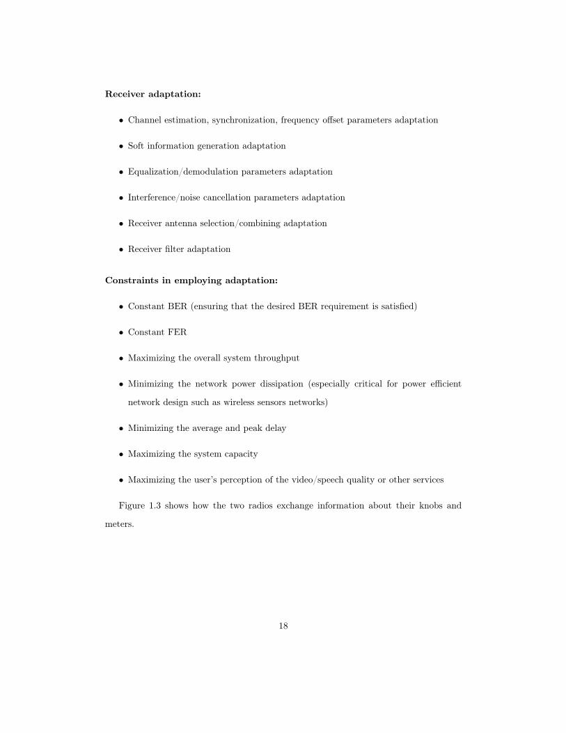
Receiver adaptation:
• Channel estimation, synchronization, frequency offset parameters adaptation
• Soft information generation adaptation
• Equalization/demodulation parameters adaptation
• Interference/noise cancellation parameters adaptation
• Receiver antenna selection/combining adaptation
• Receiver filter adaptation
Constraints in employing adaptation:
• Constant BER (ensuring that the desired BER requirement is satisfied)
• Constant FER
• Maximizing the overall system throughput
• Minimizing the network power dissipation (especially critical for power efficient
network design such as wireless sensors networks)
• Minimizing the average and peak delay
• Maximizing the system capacity
• Maximizing the user’s perception of the video/speech quality or other services
Figure 1.3 shows how the two radios exchange information about their knobs and
meters.
18
Page 34
RF
Global Policy Repository
Policy Conformance Reasoner
Local Policy Repository
System Strategy Reasoner
Policy Enforcer
Radio Platform
Sensor
RequestOpportunities
Allow/Deny
Data Source/Sink
RF
Global Policy Repository
Policy Conformance Reasoner
Local Policy Repository
System Strategy Reasoner
Policy Enforcer
Radio Platform
Sensor
RequestOpportunities
Allow/Deny
Data Source/Sink
Transmitter Receiver
Knobs & Meters of Tx
Meters of Rx
Knobs of RxKnobs of Tx
Knobs & Meters of Rx
Meters of Tx
Figure 1.3: Architecture of Two Cognitive Radios
1.5.2 Control Model
There are different control models to describe the control mechanism of the cognitive
radio. Figure 1.4 shows an example of the closed-loop feedback control model. In this
model, the system is split into a controller, a plant and a QoS subsystem. Recalling the
cognitive radio architecture in Figure 1.1, we can think of the SSR as a controller. The
controller calculates the knobs as a function of the goal and the observed meters. Then,
the plant, being the actual operational part of the radio, takes the knobs and other sensed
information from the environment. The observed meters from the plant are collected by
the QoS subsystem. Based on the goal of the application, the QoS subsystem calculates
the QoS based on the meters. The QoS reflects the overall performance of system and
goes to the controller as a feedback. The controller then evaluate whether the goal is
achieved. If not, then the controller will change its input (knobs) to the plant to achieve
the control goal [18].
19
Page 35
Controller(SSR)
Plant(Radio Platform) QoS
Goal Knobs Meters QoS
EnvironmentEnvironment
Figure 1.4: Example of Cognitive Radio Control Model
1.6 Dissertation Organization
This dissertation is organized as follows. In Chapter 2, we formulate the link adaptation
problem. Chapter 3 reviews the pertinent literature. In Chapter 4, we discuss the design
options to solve the link adaptation problem and then propose an ontology and policy
based approach. Chapters 5 - 6 present the ontology radio ontology and the policies
in details. In Chapters 7 - 8, we show the results of the MATLAB simulation and the
implementations on GNURadio. At the end, we evaluate the benefits and costs of the
ontology and policy based approach in Chapter 9.
20
Page 36
Chapter 2
Link Adaptation: Problem
Formulation
As was stated in Section 1.3, a cognitive radio is expected to have a number of capabili-
ties. Some of these capabilities, like spectrum sensing, are currently actively pursued by
various SDR projects. However, the capabilities of reasoning, especially combined with
adaptation, has not been reported in the literature. For this purpose, this thesis focuses
on the adaptation of communications link.
A wireless communications link consists of a transmitter-receiver pair, and the wire-
less medium via which information is transferred. The general goal of link adaptation is
to maximize the information bit rate per transmitted watt of power subject to a set of
constraints. This is attained by fine-tuning the parameters in the transmitter and the re-
ceiver, while the channel parameters are assigned with approximate values by estimation.
2.1 Description of Communications Parameters
Before introducing the of the adaptation problem we are going to solve, we will first take
a look at the parameters associated with the transmitter, the receiver and the channel.
21
Page 37
For each parameter, its symbol and its default value is shown. Some of these parameters
are constant throughout a communications session, while some others may be either used
in the estimation of other parameters or for controlling the communications link. These
parameters are used in the MATLAB simulation code [49].
2.1.1 Channel Parameters
• fd = 0.0001
This variable is the Doppler frequency and corresponds to the frequency offset between
the receiver and the transmitter. It has units of cycles per sample period.
• mdp = [10, 0.20, 0.010, 0.001]
This row vector contains the multipath information for the link. Each component rep-
resents the variance of each path’s quadrature component. The delay between paths is
equal to the channel symbol period divided by the transmitter variable fracSpacing. The
default value of fracSpacing is equal to 2. Each path is a complex Gaussian random pro-
cess, each quadrature component of which has an exponential covariance function. mdp
is estimated at the receiver, using previous packet transmissions from the transmitter.
• varnoise = 0.01
This is twice the variance of each quadrature noise component, per sample.
• distortflag = 0
This is a flag: 1 denotes the existence of distortion via noise and multipath, while 0
denotes no distortion.
• cohtime = 10, 0000
Coherence time is the time over which a propagation wave (the signal) may be considered
coherent (constant). This is approximately 5 times the 3dB channel coherence time (aka
Memory) in samples, and controls the rate of change of the channel taps. cohtime is
estimated at the receiver using previous packet transmissions from the transmitter.
22
Page 38
2.1.2 Transmitter Parameters
• maxmsglen = 100
This parameter controls the maximum size of an ASCII message, in characters.
• payloadsize = 128
This is the size of message field plus control field. This is referred to as the payload, and
is passed to the CRC encoding routine.
• m = 3
This is the integer index for the (2m−1, 2m−1−m) Hamming code. That is, the number
of information bits per codeword is 2m − 1−m, and the codeword length is 2m − 1. The
index must be 2 or higher. Note that the coding overhead is given by: m/(2m− 1). Since
a Hamming decoder can only correct a single error in 2m−1 received bits, as m increases,
the ratio between the size of overhead and the size of the whole packet decreases. There
is no natural upper bound of m.
• trainPeriod = 100
This is the length of the training sequence, in channel symbols.
• fracSpacing = 2
This is the number of samples per channel symbol. It is usually not changed.
• v = 1
This is the positive integer which controls the size of the QAM constellation, which is 4v.
The number of coded bits per symbol is 2v.
• packetid = 2
This is the packet ID, which is incremented by units.
• nextACKid = 1
23
Page 39
This is the ID of the packet to be acknowledged in the current transmission. The ARQ-
policy is stop-and-wait, so the other radio will retransmit packet nextACKid if it is not
acknowledged.
• PowdB = 0
This is the transmission power measured in dBm.
2.1.3 Receiver Parameters
• M = 2
This the positive integer number of feedback taps in the equalizer.
• N1 = 1
This is the positive integer number of precursor feedforward taps.
• N2 = 1
This is the positive number of postcursor feedforward taps. The general rule for specifying
M , N1, and N2 are:
N1 +N2 = length(mdp) (2.1)
M =N1 +N2
fracSpacing(2.2)
Larger values are also acceptable, but the length of the shortest training sequence is
approximately 5 ∗ (N1 +N2 +M).
• fracSpacing = 2
This is the number of (receiver) samples per symbol. It is usually set to 2.
• Memory = 100
This is the number of samples over which the channel is assumed to be constant. It is
used to train the equalizer coefficients. It should never exceed cohtime5 (if known), as the
24
Page 40
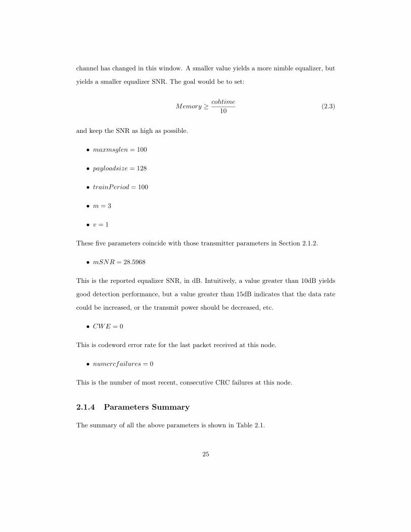
channel has changed in this window. A smaller value yields a more nimble equalizer, but
yields a smaller equalizer SNR. The goal would be to set:
Memory ≥ cohtime
10(2.3)
and keep the SNR as high as possible.
• maxmsglen = 100
• payloadsize = 128
• trainPeriod = 100
• m = 3
• v = 1
These five parameters coincide with those transmitter parameters in Section 2.1.2.
• mSNR = 28.5968
This is the reported equalizer SNR, in dB. Intuitively, a value greater than 10dB yields
good detection performance, but a value greater than 15dB indicates that the data rate
could be increased, or the transmit power should be decreased, etc.
• CWE = 0
This is codeword error rate for the last packet received at this node.
• numcrcfailures = 0
This is the number of most recent, consecutive CRC failures at this node.
2.1.4 Parameters Summary
The summary of all the above parameters is shown in Table 2.1.
25
Page 41
No. Transmitter
Parameters
Receiver
Parameters
Channel
Parameters
Notes Fixed/ Estimated/
Measured/
Negotiable
1 fd=0.0001 (cycles
per sample period)
Estimated
2 mdp=[10, 0.20,
0.010, 0.001]
Estimated
3 varnoise=0.01 Estimated
4 distorflag=0 Measured
5 cohtime=10,0000
(sample)
Estimated
6 maxmsglen=100
(character)
maxmsglen=100
(character)
maximum size of an
ASCII message
Fixed (=100)
7 payloadsize=128
(byte)
payloadsize=128
(byte)
payload = message
field + control field
Fixed (=128)
8 m=3 m=3 (2^m-1, 2^m-1-m)
hamming code
Negotiable
9 trainPeriod=100
(channel symbol)
trainPeriod=100
(channel symbol)
Negotiable
10 fracSpacing=2
(number of samples
per channel
symbol)
fracSpacing=2
(number of samples
per channel
symbol)
Fixed (=2)
11 v=1 v=1 4^v is the size of
QAM constellation
Negotiable
12 packetid=2
13 nextACKid=1
14 PowdB=0 (dB) Negotiable
15 M=2 number of feedback
taps in equalizer
Negotiable
16 N1=1 number of
precursor
feedforward taps
Negotiable
17 N2=1 number of
postcursor
feedforward taps
Negotiable
18 memory=100
(sample)
Negotiable
19 mSNR=28.5968
(dB)
Measured
20 CWE=0 codeword error rate Measured
21 numcrcfailures number of most
recent, consecutive
CRC failures at
this node
Measured
+
Table 2.1: Parameters Summary
26
Page 42
2.2 Objective Function
In this link adaptation problem, the goal is to maximize the information bit rate per
transmitted watt of power. The computation of information bit rate is shown as follows.
The payload size is fixed per packet to be payloadsize·8 information bits. “Information
bits” means the bits comprising the message, the control field, and any padding. These
bits are passed into a CRC32 checker which postpends 32 bits. The result is then coded
in the following way:
• (32 + payloadsize · 8) is padded so that the number of bits is evenly divided by
2m −m− 1. We neglect this in the calculation.
• The bit stream is coded to yield approximately
(32 + payloadsize · 8)(1 +m
2m −m− 1) (2.4)
coded bits.
• The coded bit stream is QAM modulated to form
(32 + payloadsize · 8)(1 + m2m−m−1 )
2 · v(2.5)
• QAM channel symbols. Again, a few additional bits are postpended to make the
new length divisible by 2v.
• QAM symbols are prepended to form the training sequence. The total number of
QAM symbols in the packet is
trainPeriod+(32 + payload · 8)(1 + m
2m−m−1 )
2 · v(2.6)
• The transmitter uses
10PowdB
10
1000 · [trainPeriod+(32+payload·8)(1+ m
2m−m−1 )
2·v ] · fracSpacingsampleRate
(2.7)
Joules of energy to send payloadsize · 8bits.
27
Page 43
• The goal is to maximize the information bit rate per transmitted watt of power,
hence the metric to maximize is
payload · 8 · sampleRate10
PowdB10
1000 · [trainPeriod+(32+payload·8)(1+ m
2m−m−1 )
2·v ] · fracSpacing(2.8)
• Suppose sampleRate, payloadsize and fracSpacing are fixed, we can minimize
10PowdB
10 · [trainPeriod+(32 + payload · 8)(1 + m
2m−m−1 )
2 · v] (2.9)
• Assume that payload is fixed to 128 bytes, the objective function can be further
simplified to
10PowdB
10 · [trainPeriod+528 · (1 + m
2m−m−1 )
v(2.10)
There are four variables in the objective function: PowdB, trainPeriod, m and v.
The increase of PowdB or trainPeriod will produce an increase of the objective function.
The increase of v or m will yield to a decrease of the objective function. Also, PowdB,
trainPeriod, and v affect the value of another variable mSNR, which will be discussed
in the following section. The range of mSNR must be from 10 to 15.
2.3 Constraints
Suppose for the nth transmission, PowdBn, mSNRn and vn are the transmission power,
signal-to-noise ratio, and the size of the QAM constellation, respectively.
1. The reported equalizer SNRn must be between 10dB and 15dB. Intuitively, a
value greater than 10dB yields good detection performance, but a value greater
than 15dB indicates that the data rate could be increased, or the transmit power
should be decreased. Hence, the constraints for mSNRn is:
10 ≤ mSNRn ≤ 15 (2.11)
28
Page 44
2. PowdB is the transmit power in dB. Here, we set the upper bound of PowdB as:
PowdB ≤ 0dB (2.12)
3. Suppose
∆PowdBn = PowdBn − PowdBn−1 (2.13)
and
∆mSNRn = mSNRn −mSNRn−1 (2.14)
Since both PowdB and mSNR are in dB, a drop of PowdB results in an equal
drop in mSNR. Thus
∆PowdBn = ∆mSNRn (2.15)
To guarantee Eq.2.11, ∆mSNRn must not exceed 15−mSNRn−1 and not be less
than 10−mSNRn−1 . Hence,
10−mSNRn−1 ≤ ∆PowdBn ≤ 15−mSNRn−1 (2.16)
that is:
10−mSNRn−1 + PowdBn−1 ≤ PowdBn ≤ 15−mSNRn−1 + PowdBn−1 (2.17)
4. The parameter m is the integer index for the (2m − 1, 2m − 1−m) Hamming code.
That is, the number of information bits per codeword is 2m − 1 − m, and the
codeword length is 2m − 1. The index must be 2 or higher. Thus the lower bound
of m is 2. The parameter m does not effect the equalizer’s SNR, as it controls the
coding overhead. There is no natural upper bound of m. However, since the length
of the overhead must be larger than zero, we can compute an approximate upper
bound ofm by assuming length of the payload is fixed. In the MATLAB simulation,
29
Page 45
payload is fixed to 128 bits, according to the discussion in Section 2.2, the length
of the Hamming code overhead equals to:
(payload · 8 + 32) · m
2m − 1−m= 1056 · m
2m − 1−m(2.18)
Here we set
m ≤ 10 (2.19)
Hence the lowerbound of the length of the Hamming code overhead approximately
equals to 10.
5. The parameter v controls the size of the QAM constellation, the natural lower bound
of v is:
v ≥ 1 (2.20)
Parameter v does affect equalizer performance, in the following way. For a given
value of v, the QAM constellation has a maximum magnitude of unity, achieved at
the corners. There are 4v points uniformly in a rectangular grid, and the minimum
distance between distinct constellation points is 1√2(2v−1) . Consequently, a possible
increase in v by 1 unit would drop the SNR by the factor ( 2v−12v+1 − 1)2, or approxi-
mately by 14v , which is 6dB 1. In short, increasing v by one unit drops the equalizer
SNR by approximately 6dB. Suppose
∆vn = vn − vn−1 (2.21)
then
∆vn = −∆mSNRn
6(2.22)
Again, to guarantee Eq.2.11, ∆mSNRn must not exceed 15−mSNRn−1 and not1In fact, since 10log4v = 6 + 10logv, the drop is 6 + 10logvdb.
30
Page 46
be less than 10−mSNRn−1. Hence,
mSNRn−1 − 15
6≤ ∆vn ≤
mSNRn−1 − 10
6(2.23)
This constraint can be further simplified to
dmSNRn−1 − 15
6e+ vn−1 ≤ vn ≤ b
mSNRn−1 − 10
6c+ vn−1 (2.24)
6. The parameter trainPeriod affects the equalizer performance in a less clear way.
If trainPeriod is less than 5 ∗ (M + N1 + N2), then the equalizer does not fully
converge. The QAM symbol detection may fail completely, or recover after an
initial burst symbol errors. Recall that our coding cannot handle error bursts, so if
trainPeriod is reduced below that critical value, CRC errors may suddenly appear.
On the other hand, making trainPeriod greater than twice the critical value will
have little effect on equalizer performance, but will work against the minimization
of the metric. Hence, the constraint of parameter trainPeriod is:
5 · (Mn +N1n +N2n) ≤ trainPeriodn ≤ 10 · (Mn +N1n +N2n) (2.25)
7. Clearly,M , N1, N2 have a threshold influence on equalizer performance: the equal-
izer SNR will increase with M , N1, or N2, until a sufficiently large equalizer for
the multipath is achieved. After that point, increasing the equalizer dimensions will
have no effect, except to increase the shortest possible training sequence.
8. The equalizer SNR will increase with the parameterMemory. Then, it flattens out,
and decrease as Memory exceeds cohtime5 as mentioned earlier. On the other hand,
a smaller value yields a more nimble equalizer. Here, the range of Memory is set
to:cohtime
10≤Memory ≤ cohtime
5(2.26)
31
Page 47
2.4 Formal Description of Link Adaptation Process
The basic adaptation process for this link adaptation problem has the following steps.
1. In the n− 1 th transmission, the values of the tunable transmitter parameters are
{PowdBn−1, trainPeriodn−1, mn−1, vn−1}, and the values of the tunable receiver
parameters are {mSNRn−1, Mn−1, N1n−1, N2n−1, Memoryn−1}. Using this set
of parameters, the transmitter sends a data packet to the receiver.
2. The receiver receives the data packet, and then run an adaptation algorithm to com-
pute the optimized values of the transmitter parameters and the receiver parameters
for the n+ 1 th transmission, i.e. {PowdBn, trainPeriodn, mn, vn, mSNRn, Mn,
N1n, N2n, Memoryn}.
3. Then the receiver sends the suggested parameters values {PowdBn, trainPeriodn,
mn, vn, mSNRn, Mn, N1n , N2n, Memoryn } to the transmitter.
4. If the transmitter accepts these suggested values, it will change its transmission
parameters accordingly. Otherwise, the transmitter will negotiate with the receiver
and repeat step 1 to 3 until they both agree on a new set of parameters values.
Basically, the link adaptation problem stated above requires that the transmitter and
receiver coordinate and negotiate with each other to find an optimized solution of the
transmission parameters. The issues regarding how they negotiate with each other and
which algorithm is used to find a optimized solution will be discussed in Section 4.3. In
this section, we are trying to deduce a formal description of the adaptation problem, i.e.
the objective function and the constraints.
Objective Function and Constraints: Suppose {PowdBn−1, trainPeriodn−1,mn−1,
vn−1 , mSNRn−1, Mn−1, N1n−1, N2n−1, Memoryn−1 } are known knobs and meters
obtained from the n−1 th transmission. {PowdBn, trainPeriodn, mn, vn, mSNRn,Mn,
N1n, N2n,Memoryn } are tunable knobs that will be optimized for the n th transmission.
32
Page 48
• Objective Function
Minimize
f = 10PowdBn
10 · [trainPeriodn +528 · (1 + mn
2mn−mn−1 )
vn(2.27)
• Subject to the following constraints:
Constraints1 10 ≤ mSNRn ≤ 152 PowdBn ≤ 03 10−mSNRn−1+PowdBn−1 ≤ PowdBn ≤ 15−mSNRn−1+PowdBn−14 N1n +N2n ≥ 4
5 Mn ≥ N1n+N2n2
6 5 ∗ (Mn +N1n +N2n) ≤ trainPeriodn ≤ 10 ∗ (Mn +N1n +N2n)
7 cohtimen−1
10 ≤Memoryn ≤ cohtimen−1
5
8 2 ≤ mn ≤ 109 1 ≤ vn10 dmSNRn−1−15
6 e+ vn−1 ≤ vn ≤ bmSNRn−106 c+ vn−1
11 Mn, N1n, N2n, trainPeriodn,Memoryn,mn, vn are integerNotes
1. mSNRn will increase with Mn, N1n, or N2n, until a sufficientlylarge equalizer for the multipath is achieved. After that point,increasing the equalizer dimensions will have no effect, except toincrease the shortest possible training sequence.
2. mSNRn will increase with the parameter Memoryn, flatten out,and then decrease as Memoryn exceeds cohtime
5
3. cohtimen−1 is a known parameter that is estimated at thereceiver
Table 2.2: Constraints of the Link Adaptation Problem
33
Page 49
Chapter 3
Literature Review
Below, several techniques that are relevant to the problem defined above are listed, fol-
lowed by an analysis of the applicability of each approach. Then, a brief introduction to
the proposed approach will be given.
3.1 Exhaustive Search
The exhaustive search systematically checks all the possible candidates in hope of finding
a solution that satisfies the problem’s goal state. It is easy to implement. However,
the cost is proportional to the number of the candidates. For example, if there are 10
tunable parameters, and each parameter has 10 possible values, the search space has 1010
possible candidates. Obviously, the exhaustive search is applicable to problems of smaller
size or when the simplicity of implementation is more important than the search speed.
However, communication systems are generally complicated with a lot of parameters. For
examples, in a real CDMA system, there can be as many as approximately 3000 tunable
parameters that can affect the performance of the communications. Exhaustive search is
not an appropriate choice in this case.
34
Page 50
3.2 Genetic Algorithms
Genetic algorithms have been proven successful in finding solutions in multi-objectives
optimization problems [3]. The basic idea is that the genetic algorithms encode a set of
input parameters that represent a possible solution into a chromosome and apply selection
and reproduction operators to “evolve” a gene that is successful, as measured by a fitness
function. The basic elements in genetic algorithms include the following:
• Fitness function
The fitness function evaluates a ranking metric of chromosome of an individual, and
determine its survival to the next generation. The individual with higher fitness is more
likely to survive. The fitness function can be done through a metric like cost or weight.
In multi-objective optimization problems, the fitness function is computed by combining
the evaluations along different dimensions into a single metric. For example, the fitness
function is given as a utility function [3]:
f =
NO∑i=1
wiln(ciλi
) (3.1)
This function computes the fitness of an individual over NO objectives. Each objective
has a credit score ci, a preference weight wi, and a normalization factor λi. The normal-
ization factor can avoid the problem that the values of the dimensions may vary greatly
in magnitude, e.g. BER of 10−6 vs. data rate of 106. The choosing of the preference
weights depends on the quality of the service goals.
• Chromosome representation
In the classic genetic algorithms approach, an chromosome is represented as a string
over a finite alphabet. Each element of the string is called a gene. The value of each
element is usually chosen from a binary alphabet, 0 and 1. In cognitive radio, “a radio
may be capable of thousands of center frequencies over multiple GHz but only has a few
35
Page 51
modulations from which to choose. The chromosome can therefore give a large number
of bits to the frequency gene and a small number to the modulation gene.” Therefore,
the bit representation of a chromosome can be very flexible. We can assign 20 bits to
represent the “Frequency” gene and 4 bits to represent the “Modulation” gene.
• Selection
The chromosome with a higher fitness is more likely to be selected and survive in the
next generation. The selection is randomized with a probability that is proportional to
the fitness. The selected chromosome will get to the reproduction process.
• Reproduction
The reproduction process includes cross-over and mutation. First of all, the selected
chromosomes will be paired up randomly, becoming the parents. Then one or more cross-
over points will be chosen randomly, which determines the position in the chromosome
where parents exchange genes. After cross-over is performed, the two parents generate
two new offsprings. Then mutation can be performed on the offspring chromosome.
Each gene can be altered by a random mutation to a different number according to the
mutation probability. If the chromosome is represented by 0 and 1, then the values of the
selected gene will be flipped. At this point, all the chromosomes for the next generation
are generated. The same processes will be performed on the next generation until a
chromosome is found with a desirable fitness value. [25, 10, 3]
3.3 Case-based Reasoning
Case-based reasoning is a method to aid the decision making process using the past
knowledge. The information observed by the sensor, e.g. the changes of the environment
or the user’s requirement can be modeled as an individual problem. Each problem has
perception, actions and results. The past knowledge can be encoded in a table that
includes the perception, action and results of each past individual problem. Here the result
36
Page 52
means how successful an action was in responding to a problem. When new information
of the environment comes in, a new problem is generated. Then the decision making
system will looking up into the table and determines the similarities between the new
problem and the past problems as well as the utility of the past actions. Then using the
similarities and utility of the case, the system selects the most representative case to the
new problem and perform the actions. Then the result of the new problem along with the
actions will be fed back to the lookup table and stored as a new problem. As the system
processes, the knowledge base becomes bigger and bigger, with more cases and actions
that better reflect the environment to help make a better decision [10].
3.4 Game Theory
In games such as chess, the two players act as two hostile agents trying to diminish one’s
well-being. Since the rules are well-defined, the players are limited to a small number of
actions. In addition, the state of the game is fully accessible to the players and easy to
be represented. Therefore, this kind of games can be represented as a search through a
space of possible game positions.
The existence of an opponent not only introduces the uncertainty of the environment.
What makes it worse is that the two players are trying their best to achieve the same
goal. In [13], a good example is shown to illustrate the cognitive radio’s dilemma. In this
example, two radios are in the same environment and trying to maximize their throughput.
Each radio can implement a narrowband waveform or a wideband waveform. There are
three available options:
(1) If both radios implement the narrowband waveform, then there is no interference
and both of them can achieve a throughput of 9.6Kbps.
(2) If one radio implements a narrowband waveform while the other radio implements a
wideband waveform, then there will be interference. The narrowband signal will achieve a
throughput of 3.2Kbps whereas the wideband signal will achieve a throughput of 21Kbps.
37
Page 53
(3) If both of the radios implement the wideband waveform, then more interference
will occur. Both of them will achieve a throughput of 7Kbps.
From the perspective of game theory, this problem can be solved by finding the Nash
Equilibrium (NE). An action vector is an NE if no player can improve its performance
by itself. In the above example, action vector (wideband, wideband) is the NE because
neither of the radios can unilaterally deviate from (wideband, wideband) to improve its
performance. For example, if radio 1 wants to improve its performance, it must either
change to (wideband, narrowband) or (narrowband, narrowband). Either of these options
requires that radio 2 change from wideband to narrowband.
In the cognitive radio network, if no radio can find an adaption to achieve better
performance, then this state is a NE. Furthermore, the network would remain in NE for
any rational decision rule.
However, the unique NE for a game may not be the desirable solution. In [13], an
example is shown where all the radios in the network are running power-control algorithm
trying to maximize the signal-to-noise radio at the receiver. The unique NE for this game
is the power vector where all the radios transmit at maximum power. Obviously this
NE is not the desirable solution when we take in account of the battery life. In such
a situation, other optimality approaches such as Markov chain theory can be used such
that the steady state can be evaluated via some appropriate network objective functions.
3.5 Expert Systems
The DENDRAL program is the first successful expert system [84, 85, 86, 87, 88, 89]. It is
an AI software in organic chemistry introduced by Edward Feigenbaum. The distinction
between traditional problem solving programs and expert system is the way the problem-
specific expertise is coded. In traditional problem solving approach, such as exhaustive
search or genetic algorithm as mentioned above, the problem related expertise is encoded
in both program and data structure. On the other hand, in expert system, the problem
38
Page 54
related expertise is only coded in the data structure. The program is independent from
the problem related expertise, i.e. there is no problem specific information encoded in
the program.
The basic architecture of an expert system includes two components: knowledge base
and inference engine. Knowledge base contains the formally encoded problem-specific
knowledge, e.g. the inference rules in the form of IF-THEN or the static facts in the form
of Triples. An inference rule is a statement that has a IF part and a THEN part. It can be
seen as a function describing the relationship between premises (IF part) and conclusion
(THEN part). The conclusion can be derived to be true if the premise holds. An inference
engine is a problem-independent program that is capable to derive implicit facts from
the knowledge base. There are two kinds of inference methods: forward chaining and
backward chaining. Forward chaining starts with the available knowledge and uses the
inference rules to derive new knowledge (implicit facts) until a goal is achieved. On the
other hand, the backward chaining starts with the goals and uses the inference rules to
see if there is any data in the knowledge base that can allow it to derive any of the goals
[25].
3.6 Ontology Based Radio
The concept of Ontology-Based Radio (OBR) was proposed by Kokar, Baclawski, Brady
and Wang in [29]. OBR uses the combination of ontology, policy and policy reasoning
to provide the flexibility and interoperability of the communication nodes. An ontology
defines the basic terms in a domain and the relationships among them. It is used to share
information among people, machines, or both in order to facilitate further analysis of the
domain knowledge. In the cognitive radio domain, two radios can achieve interoperability
by exchanging the knowledge about their communication parameters and protocols. The
knowledge, which includes information like the capabilities, configuration and system
state of the radio, can be used to reconfigure the radios in a flexible way. Policies are sets
39
Page 55
of rules about how to change the behavior of the radios. A policy reasoner is a component
capable of deductive reasoning over the ontology and the rules.
OBR has the following features. First, all the internal/external information and the
signaling messages are represented in the Web Ontology Language (OWL). OWL is a
formal language with high expressivity and computer processable semantics and there-
fore is capable of expressing complicated information and can be processed by the in-
ference engine. Second, the operation of OBR is controlled by some policy rather than
device-specific software embedded into hardware, i.e. we can define and change the radio
operation by changing the policy during its operation.
In [29], an experimental implementation of OBR was constructed where two radios
used ontology-based reasoning to determine the length of the equalizer training sequence.
In the experiment, the ontology written in OWL was first converted to a Prolog program,
which was in turn processed using Kernel Prolog, a Java based Prolog interpreter.
Bearing the same concept, the Modeling Language for Mobility (MLM) working group
in the Wireless Innovation Forum is leading an effort to develop a formal language, with
computer understandable semantics, that could be used to describe all aspects of network
operations and management [61, 58, 63, 62]. Papers [23] and [53] discuss the language
issues that arose in the process of developing the ontology and policies for cognitive radio.
In [65], we use a public safety use case to demonstrate how to combine ontology, policy
and inference engine to control the radio behavior. In addition, the IEEE P1900.5 working
group is making an effort to define a policy language to specify interoperable control of
the cognitive radio functionality.
40
Page 56
Chapter 4
Design Options and Proposed
Solution
To propose an approach to solve the link adaptation problem, a number of design options
will be evaluated in this chapter. First we will compare the knowledge-less and knowledge-
based approaches that have been reviewed in Chapter 3. Second, we will discuss the
languages that can be used for the implementation of the adaptation scenarios (see Section
4.2). Moreover, language candidates for representing ontologies are briefly discussed.
Third, we will compare the collaborative and non-collaborative approaches. Fourth, fixed
protocol approach versus flexible signaling will be evaluated. Finally, we will propose an
approach to solve the link adaptation problem.
4.1 Knowledge-less vs. Knowledge-based Approaches
It is important to clarify the distinction between information and knowledge. Information
is the raw data of the environment collected through sensors, e.g. interference, battery life,
position. The information can be used as the input of the adaptation or learning routine
and help them make decision. On the other hand, knowledge is a useful representation of
41
Page 57
information that can be used to interpret the information [3]. For example, a sensor can
collect the time and location information and provide them to the cognitive radio. This
information is useless to the radio unless the radio knows what that information means
about the potential use pattern, e.g. area of outage or high interference at a regular time
of the day. Knowledge is used in logical reasoning for generating new knowledge from
existing knowledge, whereas information does not have such an capability.
The approaches listed in Chapter 3 can be classified into two categories: knowledge-
less approach and knowledge-based approach.
In the knowledge-less approach, such as exhaustive search and genetic algorithms, the
percepts from the environment are represented as information rather than knowledge.
For example, in Rondeau’s wireless system genetic algorithm (WSGA) approach [3], the
input information is a list of tunable knobs and the range of each knob. He used a XML
file and a DTD file to represent this information. The XML file is used to provide the
bounds, step size and the number of bits of each knob, whereas the DTD file provides the
minimum representation of the waveform to structure the chromosomes. The information
provided by the XML and DTD files is used to generate the chromosomes in the search
space. The size of the search space can be reduced by various techniques, e.g. mapping
to a feature space or using heuristics to cut some branches. Then the search algorithm
will try to find the solution in the search space. It is worth mentioning that though XML
is capable of capturing the domain knowledge, e.g. subclass/superclass relationships, it
does not have the reasoning capability. Therefore, we put Rondeau’s approach into the
knowledge-less category. The details of knowledge representation will be discussed in
Section 4.2.
On the other hand, the knowledge-based approach, such as expert systems, represents
the input information as knowledge. This approach requires the creation of a “knowledge
base” that captures the domain knowledge and represent it in a formal way so that the
knowledge is processable and understandable by the machine. Then the search algorithm
(embedded in the inference engine) will search the knowledge base and try to find a
42
Page 58
solution. The success of a knowledge-based approach depends on whether the human’s
knowledge of the problem is good or bad. If the problem-specific knowledge is abundant,
then the knowledge-based approach is likely to perform well. The most successful expert
systems application usually result from the fact that the human approach to solving the
problem is already well understood by domain experts and stabilized [1].
The most distinguished benefit of the knowledge-based approach is its reasoning capa-
bility. The reasoning capability enables it to combine knowledge gained at different times
in different places and infer the implicit facts from the knowledge base. The implicit
facts can be used to aid the decision making. Take the link adaptation problem as an
example. The input of the system is the knobs and meters from the n − 1 th transmis-
sion: {PowdBn−1, trainPeriodn−1, mn−1, vn−1, Mn−1, N1n−1, N2n−1, Memoryn−1,
mSNRn−1, distorflagn−1, CWEn−1 }. The knowledge-less approach only takes these
parameters as unrelated input data and is not able to infer what that information implies
to the radio. On the other hand, the knowledge-based approach can infer the implicit
relationship among these parameters and the state of the radio, then use this information
to help the adaptation process.
When the search space is small, the knowledge-less approach can also infer some
kind of simple implicit information by adding a few rules (IF/THEN statements) in the
algorithm. However, in the CDMA system, there can be about 3000 tunable knobs. It is
not feasible to write thousands of IF/THEN rules for each combination of the parameters.
The knowledge-based approach is more preferable in such cases, because this approach
represents the relationship among information, e.g. subclass/superclass and it is possible
to write generic inference rules rather than specific rules for each parameter. In addition,
formal inference has no limit to the complexity of the sentences it can handle [25]. For
example, given a knowledge base (KB) of a conjunction of thousands of sentences of
facts, such as the laws of gravity and the state of objects in the solar system, the formal
inference mechanism can deal with sentences of the form “if KB then P” where P is a long
description of the eventual departure of Pluto from the system [25].
43
Page 59
In addition, in most of the knowledge-based approaches, the behavior of the radio
is controlled by rules/policies. The modification of the radio behavior becomes more
flexible. The details of this issue will be addressed in Section 4.2.3.
Despite the many benefits described above, it is important to point out one acknowl-
edged shortcoming of the knowledge-based approach – new rules must be added by domain
experts as the problem set evolves, and hence the knowledge-engineering bottleneck exists
[1]. Also, the knowledge-based approach requires a large storage capacity, which may be
a serious issue for a small-size radio.
4.2 Language Selection for Ontology-Based Radio
From the perspective of Artificial Intelligence (AI), a cognitive radio can be interpreted
as a cognitive agent. The definition of such a cognitive agent is given [43] as “a cognitive
system that can be aware of the external communication environment and internal state
and then make decisions about the operating behavior to achieve the goal.” In more
detail, the cognitive radio must be able to:
1. be aware of its own capabilities and reflect on its own behavior
2. explain itself and tell other radios and network what it knows and what it wants
3. can reason about the implicit facts using the explicitly represented knowledge
4. can learn from its experience to improve the performance in the future
5. can respond robustly to surprise, i.e. react to the circumstances it has not seen
before.
All the requirements mentioned above call for a language that (1) can represent the
knowledge of the cognitive radio domain and (2) can control the radio behavior to realize
the requirements from different actors, e.g. consumers, first responders, service providers,
manufacturers, lawmakers, etc. There is agreement that a language must be accreditable,
44
Page 60
unambiguous, extensible, and interoperable. Currently, there are different IT communities
working on developing such a language, e.g. IEEE 1900.5, E2R, and SDR MLM working
group. Figure 4.1 shows a conceptual view of where standardized languages may play
a role in the communication among various actors [66]. The actors are shown at the
outside of the figure. These are the individuals and organizations that are interested in
communicating with regard to many issues. Examples of such issues are shown in the
ovals, e.g. HW/SW portability, channel frequency modulations, etc. The intermediate
layer shows some languages that the actors could possibly use. The SDRF is working on
a formal language with computer processable semantics that could be used as a common
language among the various automated processes used by the actors to address their
communications and networking needs.
Dynamic Spectrum Access (DSA) is one of the issues of interest to Regulators as well
as End Users, who in this case might be represented by the software agents running on var-
ious mobile devices. A number of emerging approaches to DSA systems employ rule-based
mechanisms to adapt radio behaviors to application needs, host system capabilities, in
situ spectrum environment, and regulatory constraints. The Defense Advanced Research
Projects Agency (DARPA) neXt Generation (XG) Communications Program proposed
the use of non-procedural computer languages and associated reasoners as a means for
expressing and enforcing sets of policies to enable and govern radio behaviors. Thus ra-
dios could roam the world while autonomously enforcing spectrum access rules according
to the policies provided by the local spectrum governing authorities. Furthermore, that
approach separates radio technologies, regulatory policies, and optimizing techniques gov-
erning spectrum access such that each of them could evolve asynchronously. As a parallel
effort, the End-to-End Reconfigurability (E2R) project is working on a markup language
for describing the functionality of various components. More recently, the IEEE SCC 41
has begun efforts to develop a set of interoperable and vendor- independent languages
and architectures for policy-based DSA systems [61].
45
Page 61
H/W, S/W
Portability Radio SW
Components
Channel
Frequency
Modulation
Spectrum
Efficiency
Cost
Effectiveness
Policy
Conformance
Load
Balancing
Quality of
ServiceHandover
SDR Forum
IEEE 802.21
IEEE
P1900
VITA 49
E2R
New
Standards
End User
Regulator
Equip
ment P
rovid
er
SW D
eveloper
Semiconductor Co.
Component Provider
Tool Vendor
Netw
ork
Opera
tor
Spectrum Broker
HandsetBase Station
MLM Language
Figure 4.1: Actors, issues and standard languages: a conceptual view (Source: [66])
Specifically, we expect the language and associated semantic reasoning mechanisms to
address the following areas as a minimum [66]:
1. Capabilities of the nodes (e.g., frequency bands, modulations, MAC protocols, ac-
cess authorizations, etiquette, bandwidths, and interconnections)
2. Networks available to a user (parameters, restrictions, costs)
3. Security / privacy (capability, constraints, policies)
4. Information types (an emergency call vs. just a “how are you” message)
5. Local spectrum situation (spectrum activity, propagation properties)
6. Network to subscriber & subscriber to network control (policies)
7. Manufacturer matters (hardware and software policy)
46
Page 62
8. Types of users (authority, priority, etc.)
9. Types of data (Async., Isoc., narrow band, broad band, etc.)
10. Local regulatory framework (e.g., policies at a given geo location, time of day,
emergency situation, etc.)
11. Time of Day (at both ends of session and important points in between)
12. Geographic Location (in three space, surrounding geography/architecture).
However, since cognitive radio is still under development, it is difficult to capture all the
requirements for all the future needs, thus there is less consensus on the expressivity and
computational modeling of such a language. In the following section, we will first talk
about the distinction between imperative language and declarative language, and then
present the available language to express ontology and policy [44].
4.2.1 Imperative Language vs. Declarative Language
Basically, computer languages can be classified into imperative languages and declarative
languages. Table 4.1 summarizes the difference between these two language types [23].
In order to decide which language fits better our needs, we need to take a closer look
at the requirements of cognitive radio.
As we have seen in the preceding section, cognitive radio must be (1) aware of the
external communication environment and internal state and then (2) make decisions about
the operating behavior to achieve the goal.
There are two concerns regarding the first aspect. First, the radio must not only be
able to be aware of the knowledge of particular facts, but also be able to understand the
implications of the facts to its operation. For example, it is not sufficient for the radio
to detect and record a dialog, but most importantly it must be capable of understanding
the content of the dialog. Another example would be spectrum awareness. If the radio
has detected an underutilized frequency, it must also know whether this frequency is
47
Page 63
Procedural/ImperativeLanguage
Declarative Language
Example C, C++, Java Prolog, SQL, OWL, SWRLAlgorithm A sequential collection of
operations/statement providesthe algorithm.
The algorithm is the inferenceengine. The input and output ofthe algorithm is provided by acollection of facts (clauses) anda goal defined by the user, e.g. a
query is the input.ControlStructure
The control structure ispartially determined by the
ordering of the operations in thelist and partially embedded inthe control statement likeif-then-else, do-while and
do-until.
The order of execution isdetermined in the way that theinference engine tries to find asolution to achieve the goal
“What” and“How”
A logic program consists of logictheory (“what”) and deduction
(“how”).The programmer needs to
specify what needs to be doneand how (in what sequence) can
it be done.
The programmer only needs tospecify what needs to be done.The “how” part is accomplished
in the inference engine.
Modification The whole program needs to bereplaced because the program is
the algorithm itself.
Only the facts (clauses) andrules need to be replaced
because they are only the input.The generic algorithm (the
inference engine) is unchanged.
Table 4.1: Imperative Language vs. Declarative Language (1)
assigned for public safety, analog TV or other usage. From this prospective, declarative
languages can satisfy the full awareness requirement. By combining an inference engine
and a declarative knowledge base that relates various variables, the radio can infer the
implication of various operating states and environment conditions. Second, the radio
is also required to be aware of its internal state. This is a feature called “reflection”
addressed by most declarative languages and some procedural languages. For example,
though a C++ program keeps values of its variables, it does not explicitly “know” its
variables. To satisfy the internal awareness, a program must be able to query about the
variables and reply about queries about its own variables, i.e., the program should be
48
Page 64
able to tell what the variables it has, the type and values of the variables [4, 23].
At this point, we will discuss the second aspect - making decisions about own behavior.
The behavior of the radio is controlled by the program’s algorithms. If all the requirements
and information are known at the design time, then this information can be hard-coded
into the program using an imperative language, which is more likely to provide better
performance than using a declarative language. Unfortunately, the programmer is not
always able to have all the information at the design time. Unexpected situation or goal
may occur, which requires the radio to respond to surprise. In such a situation, using a
declarative language is a better solution because all the information in the knowledge base
can be used to facilitate the inference engine to search for the best answer to an unexpected
query. Conversely, due to the fixed control structure of the code, the procedural approach
is not able to find an answer to an unexpected question. Furthermore, as shown in Figure
4.2, in the declarative paradigm, if a program requires modification while it is running,
we only need to change the logic rather than the algorithm itself (the algorithm is in
the inference engine). On the other hand, in the procedural paradigm, the sequencing of
the operations in the algorithm (the program) needs to be changed, which is much more
difficult to achieve, compared to the declarative approach [23].
For the above reasons, we can come to the conclusion that a declarative language
provides a better fit for the language requirements of cognitive radio.
49
Page 65
Data Program A
Program B
Data
Data
Data Program A Data
Axioms A Axioms B
Algorithm- Operations- Control(Sequencing)
Modification:- Operations- Sequencing
Procedural/Imperative
Declarative Algorithm- Logic- Control(Sequencing - responsibility of Inference Engine)
Modification:- Logic
Figure 4.2: Imperative Language vs. Declarative Language (2)
4.2.2 Ontology Language
The next question is - which declarative language to choose? There are different kinds
of declarative languages. The cognitive radio requires that the language must be ma-
chine processable and understandable. In other words, the language must be a formal
declarative language with formal syntax and semantics.
There are two kinds of knowledge that needs to be represented using such a formal
declarative language: (1) the shared concepts between radios and networks; (2) the rules
and policies that are used to control the behavior of the radio.
The shared concepts between radios and network are defined in common ontologies.
In philosophy, ontology is the study of the nature of being or existence. The concept of
ontology can be further extended to artificial intelligent, computer science and information
science. Generally, it refers to a formal, explicit specification of a set of concepts in a
50
Page 66
specific domain and the relationships between these concepts. The term formal means
that the ontology is machine processable for the purpose of knowledge reuse and sharing
[19].
In the cognitive radio domain, whenever a transmission is requested, there are at least
three things that need to be expressed in ontology: (1) the capabilities of the radio, (2) the
current environment of the radio and (3) the characteristics of the requested transmission.
Since different domains use different vocabularies, the use of ontology makes it possi-
ble to exchange information between radio agents across different organizations, providing
a shared understanding of common domain. For example, by sharing a common ontol-
ogy, the system strategy engine (SSE) maker, policy engine implementer, and regulatory
policy author can consistently and unambiguously refer to the radio parameters and the
relevant properties of the current radio environment such as frequency, power, location
and signal characteristics [44]. In some cases, the adaptation is not only based on the local
parameters but also on the parameters of the channel and other radios in the network.
Hence, the use of ontology enables interoperability between radios and further facilitates
multi-criteria adaptation on the network-level.
Ontology can be classified into static facts and dynamic facts. Static facts, usually
referred as “T box”, are the basic terms in a specific domain, usually including classes
and properties. Dynamic facts, usually referred as “A Box”, are the facts only available
as the radio is operating. They are usually the instances of the classes defined in T box.
The AI community has reached an agreement that a common language is needed to
represent ontology. The most popular candidates include the Unified Modeling Language
(UML) from the software engineering community and theWeb Ontology Language (OWL)
from the semantic web community. So far, the OWL has collected largest number of
practitioners and supporters and the semantic web community is working on various ways
to modify the expressivity of OWL. For the above reason, we adopt OWL as the ontology
representation language for cognitive radio. Though OWL has its limits on expressivity,
there are other approaches to augment the expressivity of OWL, e.g. augment OWL with
51
Page 67
rules [23].
4.2.3 Policy Language
In order to control and guide the behavior of a cognitive radio, a policy language is
desirable for representing the rules and policies. A rule is an if-then statement, i.e. if a
hypothesis is true, then the conclusion holds. Policy is a set of rules specified in declarative
form with unambiguous semantics; it is also referred to as the “R Box”. Policy engine
is a software component that reasons with policies so that a particular communication
device, or network of devices, obeys a given set of policies during its operation. Policy
can be either external policy such as the frequency bands at specific location authorized
by FCC (stored in the Policy Conformance Reasoner) or internal policy for performance
optimization (stored in the System Strategy Reasoner). The external policies are usually
written by the regulator. The goal of regulatory policy is to specify the permissible
transmission behavior of the radio, i.e. to describe conditions under which transmission
is allowed. This kind of policy is not interested in the implementation details. Conversely,
the internal policy usually concerns about how to improve the performance of the radio.
For example, a reduction of battery power may affect the ability to support multiple
waveforms or to provide sufficient transmission power. An internal policy can be used to
select and disable a low-priority waveform in order to save battery power and maintain
support to the high-priority tasks.
In the policy-based approach, policies are separated from the implementation, which
yields the benefits in the following aspects [14, 28]:
• The separation of policy and typical radio code enables the policy to be represented
on a more abstract level and with an easier understandable semantics. In the current
radios, policies are hard-coded into the radio and form an inseparable part of the ra-
dio’s firmware. They are usually programmed using imperative language such as C,
C++ and java. These languages do not have an easily understood semantics and are
52
Page 68
not expressive enough to generally specify regulatory policies. Regulatory policies
should be on a higher level than typical radio code and free from implementation
details. As we’ve mentioned in the preceding section, policy is usually represented
in a declarative language, which usually has an easier understood semantics and
makes it easier to grasp the meaning of the policy.
• The policy-based approach decouples the definition, loading and enforcement of
policy from device-specific implementations, which makes the certification process
simpler and more efficient. The policy engine, policy and device can be accredited
separately. The policy engine and each policy only need to be certified once and
then loaded to any device without additional certification. A change to a component
can be certified without accrediting the entire system. In this way, the cost of
certification is shared across the network.
• The modification of the radio behavior becomes more flexible in a policy-based
approach. For example, if a new policy is defined to adapt to a changing situation,
the new policy can be dynamically loaded without recompiling any software on the
radio.
• The policy-based approach can enable the policy and device to evolve independently,
i.e., the radio technology can be developed in advanced of policies or vice versa.
Policy languages for cognitive radio have attracted interest in several radio and IT commu-
nities in the following aspects: (1) Spectrum Management (e.g. DARPA’s XG and CoRaL
radio policy languages), (2) Information Assurance and security, (3) Network Manage-
ment (Strassner’s DEN), and (4) Configuration Management (E2R and E3). However,
there is no consensus on a common policy language so far [44].
For our experiments, we mainly used BaseVISor as the inference engine (policy engine)
because the BaseVISor policy language is relatively simple and suitable for small scale
experiments. In the BaseVISor rule language, both heads and bodies are expressed as
triples. The triple-based rules are added to the rule base and then compiled into a Rete
53
Page 69
network, generating the nodes of the Rete network. Running the Rete network causes the
rules to fire and facts to be added to the fact base. A particular rule is triggered when
the triple patterns in the body of the rule mach the facts found in the fact base. The
head of one rule may feed the body of another rule. Hence, the behavior can be flexibly
controlled by the rules.
4.3 Non-Collaborative Adaptation vs. Collaborative
Adaptation
The link adaptation can be done locally or in a collaborative way. Recall that the ob-
jective is to minimize Eq. 2.27. The four parameters in this objective function are the
tunable knobs of the transmitter. The constraints require that the measured mSNR at
the receiver must be between 10dB and 15dB. The mSNR is affected by the trans-
mitter knobs {PowdB, trainPeriod, v} and the receiver knobs {Mn−1, N1n−1, N2n−1,
Memoryn−1}. In order to satisfy themSNR constraint, the transmitter has two available
options.
1. Collaborative adaptation. The transmitter will first send a packet and wait for
a feedback of the mSNR value from the receiver. If the mSNR is not within
the desirable range, the transmitter can adjust its parameters and try to send the
packet again until mSNR constraint is satisfied. Suppose each of the parameters
{PowdB, trainPeriod, v} has two available values, then the transmitter has to try
at most 23 = 8 times until it gets a satisfactory mSNR feedback. In this approach,
the transmitter probes into the environment with a candidate solution and then
waits for a feedback for that candidate. It will try and fail repeatedly until it finds
a solution. The shortcoming is that the probing is not time-efficient. But on the
other hand, the mSNR is more accurate because it is obtained by measurement
rather than estimation. This approach will benefit most in the environment that is
54
Page 70
difficult to model, e.g. the estimation of mSNR is not available.
2. Non-collaborative adaptation. The transmitter can use an estimation of themSNR,
i.e., mSNR = f(PowdB, trainPeriod, v), and then try to search a solution on its
own without probing into the environment. This approach requires less time, but
the prerequisite is that the model of the environment is accurate and available.
Though the value ofmSNR has dependency on {PowdB, trainPeriod, v,m}, it is difficult
to express mSNR in a close-form formula, i.e. mSNR = f(PowdB, trainPeriod, v,m).
Hence, due to the lack of accurate environment model, collaborative adaptation is more
preferable in this link adaptation problem. It is worth mentioning that in the cases where
the environment model is partially known, a hybrid of the above two approaches can be
used.
If collaborative adaptation is used, then both the transmitter and the receiver partic-
ipate in the decision making process. Hence, each radio needs to collect the informations
of its own as well as the information on the other side of the link.
From the receiver’s point of view, the percepts from the environment include the knobs
of the transmitter and receiver as well as the meters obtained from the receiver. Table
4.2 summarizes the description of the percepts, actions, goals and environment of the
receiver.
The collaborative adaptation involves collaboration strategy. The collaboration strat-
egy varies depending on the goal and constraints, e.g., time constraints, power consump-
tion, etc. Figure 4.3 shows the sequence diagram of an example collaboration strategy
between two radios.
There are other possible collaboration strategies. For example, the game theory ad-
dresses the issue of how to find an optimized solution that maximizes the overall per-
formance (utility function) of the two radios. However, the prerequisite in game theory
is that the two radios are in a hostile relationship, i.e., they are trying to achieve the
same goal. For example, the two radios are competing for the same spectrum resource.
55
Page 71
Agent Type ReceiverPercepts Knobs from the n− 1 th transmission: {PowdBn−1,
trainPeriodn−1, mn−1, vn−1, Mn−1, N1n−1, N2n−1,Memoryn−1 }
Meters from the n− 1 th transmission: {mSNRn−1,CWEn−1 }
Actions Decision on the new configurations of knobs for the n thtransmission: {PowdBn, trainPeriodn, mn, vn, Mn,N1n, N2n, Memoryn }
Goals Maximize the information bit rate per Watt power (Eq.2.7)Simplified objective function: minimize Eq. 2.27
Environment Wireless channel
Table 4.2: The Description of the Percepts, Actions, Goals and Environment for the RadioAgent in the Link adaptation Problem
Tx Rx
3: Send a data packet along with the Tx knobs {PowdB_n-1, trainPeriod_n-1,m_n-1, v_n-1}
2: Compute initial Rx knobs {M_n-1, N1_n-1, N2_n-1, Memory_n-1}
5: Send nth Tx knobs {PowdB_n, trainPeriod_n, m_n, v_n}
1: Compute initial Tx knobs {PowdB_n-1, trainPeriod_n-1,m_n-1, v_n-1}
4a: Measure Rx meters {mSNR_n-1}4b: Compute the nth Tx/Rx knobs {PowdB_n, trainPeriod_n,m_n, v_n, M_n, N1_n, N2_n, Memory_n}
Figure 4.3: Sequence Diagram of Collaborative Link Adaptation
56
Page 72
Obviously, this is not the case in our link adaptation problem. However, if our problem
is extended to multi-objectives adaptation that involves competition, game theory is still
a powerful tool to use.
4.4 Fixed Protocol vs. Flexible Signaling
To achieve collaborative adaptation discussed in Section 4.3, the adaption process shall
involve collecting information from other radios and working with them to achieve the
adaptation goal. It requires (1) a proper way to exchange control information (control
messages, also referred to as signaling) between the radios, and (2) a proper way to
interpret and execute the incoming control messages. The control messages shall be
capable of expressing more aspects than the current protocols can provide. For instance,
instead of querying for a scalar parameter, cognitive radio shall also be able to inquiry for
more complicated information, such as the structure of a radio component or the finite
state machine of a component. In addition, the way to interpret and execute the incoming
control messages is expected to be flexible and efficient.
There are three possible ways to achieve collaborative adaptation [59].
1. Fixed Protocol: The first one would be to develop a communications protocol that
is capable of expressing a wide range of aspects in wireless communications (flexible
signaling). On the one hand, it would increase the size of the header of the physical
layer packets; on the other hand, it would be limited by the size of the header and
the types of information that could be included in the header. Additionally, at the
design time, it is not possible to anticipate all the future needs, and therefore the
coverage of the possible message types is still limited.
2. Flexible Signaling (XML-encoded message): The second way would be to
define a large vocabulary of control messages expressed in XML and include such
messages in the payload of the packet. This approach provides more flexibility
in that it can express more complicated signaling information, however, it would
57
Page 73
require an XML schema to provide the description of the XML structure and pro-
cedural code to interpret the control messages written in XML.
3. Flexible Signaling (OWL-encoded messages): The third approach would be
to give radios a formal language with computer-interpretable semantics in which
any control message can be encoded, provided that it can be expressed in terms of
ontology shared by the radios. This approach does not require a separate proce-
dural code to interpret each type of control messages; instead it requires a generic
interpreter, i.e., an inference engine or reasoner, to process the control messages
written in a formal language such OWL (Web Ontology Language) or RDF (Re-
source Description Framework).
Compared to the first approach, the XML and OWL approaches are both very flexible
in terms of the number of possible message types. Practically, there is no limitations of
what type of messages can be exchanged. When we need to make a change, in the XML
approach one has to modify two things: the procedural code to process the XML file and
the XML schema. In contrast, the OWL approach only needs the change of the ontology
shared by the radios. In terms of inference capabilities, XML only has syntax and does not
have formal semantics, therefore it cannot be processed by inference engines. Conversely,
OWL has formal syntax and semantics and therefore can be processed by the inference
engines.
In conclusion, flexible signaling can bring a great flexibility to the existing protocols,
i.e., an existing protocol can be extended by including an OWL-encoded control message
in the payload of the packet without much change of the preamble frame structure.
4.5 Summary of the Proposed Solution
In summary, the approach to solve the link adaptation problem has the following require-
ments:
58
Page 74
1. Knowledge-based. All the information in the radio and the environment must be
represented as knowledge in a formal way. Based on the knowledge, the radio must
be able to reason about the implicit facts, query its own parameters and other
radio’s parameters, and respond to the queries.
2. Policy-based. Each radio should have policies that can be interpreted by a rea-
soner. The policies should establish rules for optimizing particular radio parameters
(knobs) based upon the values of other parameters (meters).
3. Collaborative adaptation. The radio must be able to exchange information and
understand the messages that have been exchanged. A hybrid of collaborative
method and non-collaborative method can be used to improve the time efficiency.
4. OWL-encoded control messages. The control messages are encoded in OWL and
will be included in the payload of the packet as needed.
Based upon the above considerations, the architecture of a policy and ontology based
cognitive radio is proposed as in Figure 4.4. This architecture is a refinement of part of
the architecture shown in Figure 1.1. It focuses on the System Strategy Reasoner. Here,
the fact that there are two kinds of messages flowing - data and control - is explicitly
shown. These messages come through the same front-end, but then need to be separated.
The control messages are extracted and passed to the SSR for further processing, while
data are passed to the Data Sink for user consumption. A similar situation occurs at the
Data Out side; data items are merged with control messages generated by the SSR.
59
Page 75
Figure 4.4: Message Flow in Cognitive Radio
60
Page 76
Chapter 5
Cognitive Radio Ontology
5.1 Overview
In order to standardize the ontology-based approach to cognitive radio, a standard Cog-
nitive Radio Ontology is needed. Towards this goal, we participated in the work of the
Wireless Innovation Forum - the MLM (Modeling Language for Mobility) Work Group,
whose goal was to come up with a standardized way of representing signaling among
cognitive radios. With the help from the MLM WG, we developed a base ontology and
submitted it as a contribution to the Forum. The CRO has been approved by the Wireless
Innovation Forum as its recommendation [58]. It is expected that the CRO will provide
opportunities for development of interoperable radios by independent vendors and lead
to specifications/standards for data exchange to support the next generation capabilities.
The Cognitive Radio Ontology (CRO) includes:
• Core Ontology (covering basic terms of wireless communications from the PHY and
MAC layers)
• Concepts needed to express the use cases developed by the MLM WG; only the use
cases that relate to the PHY and MAC layers are included
61
Page 77
• Partial expression of the FM3TR waveform (structure and subcomponents, FSM)
• Partial expression of the Transceiver Facility APIs
5.2 Principles of Modeling
5.2.1 Top-Level Classes
An upper ontology defines the most general concepts that are the same across different
domains. Choosing an appropriate upper ontology as a reference model is beneficial
since this will help merging different ontologies into one so that the common classes and
properties (relations) are mapped correctly.
From among the well-know upper level ontologies, we chose DOLCE, the Descriptive
Ontology for Linguistic and Cognitive Engineering [21], as our reference model. DOLCE
is based on the fundamental distinction between Endurant, Perdurant and Quality.
Endurant, also known as Object in our ontology, refers to the entity that is wholly
presented at any given snapshot of time. Examples include material objects such as a
piece of paper or an apple, and abstract objects such as an organization or a law.
Conversely, Perdurant, also known as Process in our ontology, is the entity that can
be presented only partly at any snapshot of time. A process can have temporal parts and
spatial parts. For example, the first movement of a symphony is a temporal part of a
symphony, whereas the symphony performed by the left side of the orchestra is a spatial
part of a symphony. In both cases, a part of a process is also a process itself.
At this point, we have identified the following relationships between Object and Pro-
cess (see Figure 5.1).
62
Page 78
Process
ObjectQuantity
UnitOfMeasure Value
hasSubprocess*
hasParticipant*
hasOutput*
subprocessOf*
hasInput*
hasCharacteristic*processQuantity*
participatesIn*
aggregateOf*
characterize*
characterize*
hasCharacteristic*
objectQuantity*
hasUnitOfMeasure* hasValue*
partOf*
Figure 5.1: Top-Level Classes of CRO
(1) An object cannot be a part of a process, but rather participate in a process. For
example, a person is not a part of running, but rather participates in running.
(2) The input and output of a process are objects. For instance, the input of modu-
lation is a signal, where modulation is a process and signal is an object.
(3) The capabilities of an object are a collection of processes. For example, a radio
has the capabilities of transmitting and receiving. Here, a radio is an object; transmitting
and receiving are processes.
(4) The characteristics of an object or a process can be represented as objects. For
instance, one of the characteristics of a transmitter is represented as TxChannelTransfer-
Function.
Qualities are the basic attributes or properties that can be perceived or measured.
63
Page 79
Qualities cannot exist on their own; they must be associated with either an object or a
process. All the qualities have values and some qualities have unit. The qualities without
units are represented as data-type properties. The qualities with units are associated
with a type of quantity.
Quantity is a representation of a property of an object. In other words, quantity is
a representation of quality. For instance, a physical quantity represents a property of a
physical object. Quantity carries three types of information: the type of the quantity
(e.g., mass, length), the magnitude of the property (typically a real or integer number)
and the unit of measurement associated with the given magnitude (e.g., [kg ], [m]). In this
ontology, quantity is a top-level class; it is further divided (sub-classified) into different
types, such as length, frequency, time, etc. Each quality is associated with a unit and a
value.
Note that there is no explicit Quality class in our ontology. Instead, we use objec-
tQuantity and processQuantity to represent the quality of an object or a process, as shown
in Figure 5.1.
There are two perspectives to representing the quality of an object or a process de-
pending on whether the quality has a unit or not. If the quality has a unit then the
quality is represented as a sub-property of object-type property objectQuantity. If it does
not have a unit then it is represented as a data-type property.
For example:
(1) hasWeight is a quality of Student; its unit is kilogram. Therefore, hasWeight is
represented as a sub-property of object-type property objectQuantity. The domain of
hasWeight is Student; the range is Weight (Weight is a sub-class of Quantity).
(2) However, studentID is a quality of Student; it is represented as a data-type prop-
erty. The domain of studentID is Student ; the range is Integer (Integer is one of the
built-in data types).
The same principle can be applied to represent a quality of a process. According to the
classification described above, the top-level classes in our ontology are shown in Figure
64
Page 80
5.1, including (1) Object, (2) Process, (3) Quantity, (4) Value, and (5) UnitOfMeasure.
5.2.2 Further Distinction: Object and Process
In this section, we are going to use some examples to further discuss the distinction
between object and process. Table 5.1 shows an example list of objects and processes.
All the examples are basic concepts within the cognitive radio domain.
Object ProcessAlphabet ChannelEncoder State ChannelCoding
AlphabetTableEntry Detector Transition DetectionChannel Modulator Event Modulation
ChannelModel SourceEncoder Action SourceCodingComponent Transceiver AIS Transceiving
Port PNCode Protocol PNCodeGenerationAgent Packet API MultiplexingGoal PacketField Method ... ...
DetectionEvidence NetworkSignal NetworkMembershipSample RoleSymbol ... ...
Table 5.1: Examples of Objects and Process
5.2.2.1 Physical Object vs. Non-Physical Object
The distinction between physical object and non-physical object depends on whether an
object has spatial qualities. All the objects exist in time; but not all of them exist in
space. The objects that exist in time and space, i.e. the ones with spatial location,
are physical objects [51]. Typically, the term physical object and material object are
interchangeable. Conversely, non-physical objects only exist in time. For instance, signal
is a physical object because it can be measured through time and space whether it is the
signal conducted in the radio or the signal radiated in space.
Channel is the physical transmission medium, though it may not be visible by hu-
man eyes, it does indeed exist in both time and space and thus is a physical object.
ChannelModel is a mathematical model that represents the characteristics of the chan-
65
Page 81
nel. Most abstract mathematical concepts such as equations, functions are non-physical
objects. Goal is the objective that an object intends to achieve. Role refers to what
position a network member has in the network, e.g. master, slave or peer. Both goal and
role are non-physical objects. Detector can refer to either physical object or non-physical
object depending on what detector refers to. If detector refers to a physical device, e.g. a
GPS as a location detector, then detector is classified as a physical object. This physical
detector is visible and tangible; it has height and mass that represent its spatial qualities.
However, detector may also refer to the software module that performs the detection
functionalities. In this case, detector is a non-physical object. The same methodology
can apply to the analysis of some other objects listed in Table 5.1. For some concepts, if
a precise definition is not given, then it is difficult to say whether it is a physical object
or a non-physical object. Therefore, in this version, we do not further distinguish object
class as physical object and non-physical object.
5.2.2.2 Object vs. Process
Example 1: Alphabet, Modulator, Modulation The relationships among Al-
phabet, Modulator and Modulation are good examples to show the relationship between
Object and Process.
Modulation is a process of varying one or more properties of a high frequency periodic
waveform, called the carrier signal, with respect to a modulating signal. It usually takes
digital signal as input and converts it to analog signal. Then the analog signal will be
transmitted to the wireless channel. The changes in the carrier signal are chosen from a
finite number of alternative symbols, which is called alphabet.
Alphabet, also known as modulation alphabet, is often represented on a constellation
diagram. A constellation diagram represents the possible symbols that may be selected
by a given modulation scheme as points in the complex plane. The coordinates of a point
on the constellation diagram are the symbol values. If the alphabet consists of M = 2N
alternative symbols, then each symbol represents a message consisting of bits. The index
66
Page 82
of each symbol value implies the bit pattern for that symbol. In real applications, alphabet
is actually a lookup table that has the index and symbol value for each symbol. Regardless
whether alphabet is a lookup table or a collection of symbols, alphabet presents itself as a
whole at any snapshot of time; alphabet is a non-physical object.
Modulator refers to either an electronic device or a software module that performs
modulation. In the former case, modulator is a physical object with input ports and
output ports; in the latter case, modulator is a non-physical object that encapsulates a
set of related functions, data and interfaces.
Example 2: Specification vs. Implementation Air Interface Specification
(AIS) refers to “the set of transformations and protocols applied to information that
is transmitted over a channel and the corresponding set of transformations and protocols
that convert received signals back to their information content” [27].
Typically, the specification of AIS is a document that establishes uniform criteria,
methods, processes, etc; therefore, it is a non-physical object. In the DOLCE taxonomy,
the specification of AIS can be further classified as a non-agentive social object, which is a
subclass of non-physical object. If two radios want to communicate with each other, both
of them should implement the processes and methods in the AIS specification, though
the details of the implementation may vary. Therefore, the implementation of AIS is a
process.
Application Programming Interface (API) is a similar concept, it refers to an abstrac-
tion that a software entity provides of itself to the outside in order to enable interaction
with other software entities. Typically, API contains the abstract description of a set of
classes and functions. The software that provides the functions described by an API is
said to be an implementation of the API. Therefore, it can be said that the specification
of API is an object whereas the implementation of the API is a process.
We use AIS and API as examples to demonstrate the difference between specification
and implementation because they have something in common. Both of them are inter-
67
Page 83
faces that provide a “standardization” to enable interaction between two objects. This
standardization is an agreement that both of the objects must satisfy.
In general, we consider the specification of such an interface as an object whereas the
implementation of this interface as a process.
In our ontology, we have both API and AIS categorized as subclasses of process. It
is assumed that the term API and AIS refer to the implementation, though the naming
may not reflect this assumption.
5.2.3 Part-Whole Relationship
5.2.3.1 Aggregation vs. Composition
In UML (the Unified Modeling Language), aggregation and composition are two differ-
ent types of association; both of them represent a part-whole relationship. There is a
distinction between aggregation and composition. Aggregation refers to the association
relationship between two classes when a class is a collection or container of another class,
but the contained class does not have a strong life cycle dependency on the container,
i.e. when the container class is destroyed, its contents are not [46, 52]. For instance,
AIS consists of one or more protocols for each layer that perform the layer’s functionality.
When the AIS no longer exists, its contained protocols are still there. Therefore, AIS
is an aggregation of protocols. Conversely, composition has a stronger life cycle depen-
dency between the container class and the contained class. When the container class
is destroyed, its contents are destroyed, too. For instance, an alphabet table has sev-
eral alphabetTableEntry, each alphabetTableEntry refers to a row in the table. When the
alphabet table is destroyed, all the rows in that table no longer exist.
In UML 2, properties (associations) are formalized in the UML meta-model using the
meta-classes Association, Property, Class and DataType. Association it is an aggregation
of two or more Property meta classes. One of the Property classes is linked with a Class
representing the domain of the association. Depending on whether the association range
68
Page 84
are objects or data types, the other Property classes are linked with either Class or
DataType meta classes. UML uses the isComposite Boolean-type meta-property of the
Property meta-class to specify that a given aggregation is composite (strong aggregation).
Since it is not possible to represent the property of a property in OWL, we use different
naming schemes to distinguish between aggregation and composition. All the aggregation
properties start with “aggregateOf” followed by the name of the range class. All the
composition properties start with “compositeOf” followed by the name of the range class.
Figure 5.2 shows an example to illustrate this.
AlphabetTableEntry
AIS
Protocol
Alphabet
aggregateOfProtocol*compositeOfAlphabetTableEntry*
Figure 5.2: Naming Schemes for Aggregation and Composition
5.2.3.2 Ordering of the Contained Entities
An instance of a class may contain an ordered collection of instances of other classes. The
order of the contained instances must be explicitly represented. For instance, a packet is
a composite of a sequence of packetField. The ordering of the packetField is defined in
the protocol. In this ontology, we use property append to represent the ordering of the
contained instances, i.e. an instance can be appended to another instance. For instance,
in the packet frame structure shown in Figure 5.3, preamble, destination address, source
address and control field are instances of packetField class. Each of the packetField is
appended to another packetField.
69
Page 85
Preamble Destination Address ... ...Control FieldSource Address
Figure 5.3: Packet Frame Structure
5.2.3.3 Examples of Part-Whole Relationship
The following examples will further illustrate how to represent part-whole relationships
in this ontology.
Example 1: Alphabet and AlphabetTableEntry In the example shown in Fig-
ure 5.4, Alphabet is a composite of AlphabetTableEntry. Both of them are subclasses of
Object. Table1 is an instance of the class Alphabet. Row1 and Row2 are instances of the
class AlphabetTableEntry. The “instance of” relation is shown with a dashed line.
Alphabet
Table1
Row1 Row2
Object
AlphabetTableEntry
compositeOfAlphabetTableEntry
compositeOfAlphabetTableEntry compositeOfAlphabetTableEntry
io
ioio
Figure 5.4: Example of Part-Whole Relationship (1): Alphabet and AlphabetTableEntry
70
Page 86
Example 2: API and Method In the example shown in Figure 5.5, instead of us-
ing “aggregateOf” or “compositeOf” that are used to represent the part-whole relationship
between objects, we use hasSubProcess to represent the part-whole relationship between
processes. In general, a process can have other processes as its sub-processes; in other
words, a process can be a sub-process of another process. For instance, an API contains
the abstract definitions of a set of methods. Both API and Method are considered as
process. An API has several methods as its sub-processes.
API
TxAPI
ConfigureTxCycle SetTxStopTime
Process
Method
subProcessOf
hasSubProcess
hasSubProcesshasSubProcess
subProcessOfsubProcessOf
Figure 5.5: Example of Part-Whole Relationship (2): API and Method
Example 3: Radio and RadioComponent The example shown in Figure 5.6 is
used to show the part-whole relationship between objects. A radio component consists of
several sub-components, such as antenna and modulator. A pair of symmetric properties,
hasSubComponent and subComponentOf, are used to represent the relationship between
them. These two properties are sub-properties of the more general property aggregateOf.
Although we could use aggregateOf to capture the part-whole relationship between com-
ponents, we would then loose the more specific information about this relationship and,
71
Page 87
consequently, we would not be able to infer that say A and B are components from the
information that they are related via the subComponentOf property.
Component
Radio
Antenna Modulator
Object
RadioComponent
subComponentOf
hasSubComponent
hasSubComponenthasSubComponent
subComponentOfsubComponentOf
Figure 5.6: Example of Part-Whole Relationship (3): Radio and RadioComponent
Example 4: Signal In some cases, the aggregateOf relationship may need to be
specialized to capture some specific aspects. For instance, in some cases an aggregate of
two things may lead to a different class membership of the aggregate even though the
particular components come from the same class. For instance, in Example 1, Alpha-
betTableEntry is part of Alphabet, but it is NOT an Alphabet. In Example 2, Method
is part of API, but it is NOT an API. And in Example 3, RadioComponent is part of
Radio, but it is NOT a Radio, however, both RadioComponent and Radio are subclasses
of Component.
On the other hand, as shown in Figure 5.7, an aggregate of two signals is also a Signal.
However, the aggregation of signals must satisfy their temporal ordering. For this reason,
the aggregateOf relation is specialized by adding another property appendSignal. The
append keyword is used in this ontology to indicate the ordering of other objects.
72
Page 88
Signal
aggregateOfSignal
Object
appendSignal
Figure 5.7: Example of Part-Whole Relationship (4): Signal
5.2.4 Attribute, Properties, Parameters and Arguments
5.2.4.1 Attribute vs. Property
There is a need for distinguishing between property and attribute (c.f. the discussion in [
]). An attribute is a feature of an object that is independent of the context that the object
is in. For instance, the size of a cup is this cup’s attribute. Conversely, the property of
an object depends on the context, for example, whether the cup is full or empty depends
on the context, thus it should be modeled as a property.
The ontology presented in this paper is formalized in OWL (Web Ontology Language)
using the Protege tool. OWL, however, does not provide any simple means for an explicit
distinction between attribute and property in the sense explained above. Take packet
field as an example. A packet consists of a sequence of packet fields. The size of a packet
field is an attribute of packet field, but whether a packet field is optional or mandatory
is a property since it depends on context in which a specific packet field is used. OWL
only provides two types of properties: (1) object-type property, which links an individual
to another individual, and (2) data-type property, which links an individual to an XML
Schema data-type value (e.g. Integer, Boolean, etc.). If we only use the features provided
by OWL, both packetFieldSize and isOptional should be modeled as data-type proper-
ties, i.e. packetFieldSize is linked to an integer value whereas isOptional is linked to a
Boolean value. [65]For this reason, we don’t distinguish between attribute and property
73
Page 89
in this ontology. All the qualities (attributes or properties) are represented as either an
object-type property or a data-type property. The terms attribute and property are thus
interchangeable.
5.2.4.2 Parameters and Arguments
The concept of parameter and argument are closely related.
In mathematics, an argument is an independent variable and a parameter is a function
coefficient. For instance, in equation aX + bY = c, variables X and Y are arguments
whereas the function coefficients a, b and c are parameters.
In computer science, parameter and argument are interchangeable.
In engineering, attributes of a system are the same as the properties of a system;
parameter usually refers to combination of properties that is sufficient to describe a system
response.
In our ontology, both parameter and argument are represented as either data-type or
object-type properties of the Method class, Process class, or Component class.
5.2.4.3 Example: Attributes and Properties of Transceiver Subsystem
Figure 5.8 shows an example of how to represent the properties and attributes of the
Transceiver subsystem.
In this figure, transmitCycle, transmitStartTime, and carrierFrequency are the proper-
ties of Transceiver ; implementAPI is an object-type property that shows the relationship
between component and API.
transmitCycle is the integer identifier that shall be set up during the creation to a
specific value, which is then incremented by one for each newly created transmitCycle.
Since it is an integer number without any unit, it is modeled as a data-type property.
The domain of this property is Transceiver ; the range is Integer, which is a built-in data
type.
transmitStartTime refers to the transmit start time of the corresponding transmit
74
Page 90
Object
Transceiver
Integer Time Frequency
Quantity
TransmitControlAPI
Process
implementAPI
carrierFrequencytransmitStartTime
transmitCycle
Figure 5.8: Representation of Properties and Attributes: Example of Transceiver
cycle. Since it has the unit of second, it is represented as an object-type property. The
domain is Transceiver ; the range is Time, which is a subclass of Quantity.
The way of modeling carrierFrequency is similar as transmitStartTime. It is also rep-
resented as an object-type property. The domain is Transceiver ; the range is Frequency.
In general, all the properties or attributes without unit of measure will be modeled
as data-type properties, the range being one of the built-in data types, e.g. Integer,
Boolean, String. Any properties or attributes with a unit of measure will be modeled as
object-type properties, the range will be one of the subclasses of Quantity, e.g. Time,
Frequency, Location. Each subclass of Quantity has a Value and a UnitOfMeasure. In
this way, we can specify the values for those properties or attributes that have units.
75
Page 91
5.3 Object
5.3.1 Alphabet and AlphabetTableEntry
Alphabet is a lookup table that participates in the Modulation process. In digital mod-
ulation, an analog carrier signal is modulated by a digital bit stream. The changes in
the carrier signal are chosen from a finite number of M alternative symbols, which is
called Modulation Alphabet or Alphabet. Each row of the Alphabet table is an instance
of AlphabetTableEntry class. Hence, Alphabet is an aggregation of AlphabetTableEntry.
The AlphabetTableEntry class has two properties: 1) hasIndex, and 2) hasSymbolValue,
as follows:
Index Symbol Value Bit Pattern (optional)0 1 + j 001 −1 + j 012 −1− j 113 1− j 10
Table 5.2: Example of Alphabet Table
A modulation alphabet is often represented on a constellation diagram. A constellation
diagram represents the possible symbols that may be selected by a given modulation
scheme as points in the complex plane. The Real and imaginary axes are often called
the in-phase (I-axis), and the quadrature (Q-axis). The coordinates of a point on the
constellation diagram are the symbol values.
If an alphabet consists of M = 2N alternative symbols, then each symbol represents
a message consisting of N bits.
5.3.2 Channel
Channel refers to the physical transmission medium between the transmitter and the
receiver. For example, in a cellular system, the transmission link between the Mobile
Station (MS) and the Base Station (BS) can be divided into (1) Forward Channel (from
76
Page 92
BS to MS) and (2) Reverse Channel (from MS to BS). Typically, both Forward and Re-
verse Channel have sub-channels for the transmission of either data messages or control
messages. For instance, in the IS-95 system, there are three types of overhead channels in
the forward link: pilot channel, synchronization channel and paging channel. The mod-
ulation, bandwidth, data rate and the multiplexing scheme of each channel are specified
in the Air Interface Specification (AIS).
The subclasses of Channel are shown in Figure 5.9. The relationships among Channel,
ChannelModel, Multiplexing and Modulation is shown in Figure 5.10.
PagingChannel
ForwardChannel
SyncChannel TrafficChannel
ReverseChannel
Channel
AccessChannelPilotChannel
isa isa isa isa isa
isaisa
isa
Figure 5.9: Subclasses of Channel
77
Page 93
Frequency
Quantity
Multiplexing
Process
Modulation
Channel
Object
ChannelModel
isa
isa
isa
isa
channelCentralFrequency*
hasModulation*
isa
characterize*participateIn*
channelBandwidth*
characterize*
participateIn*
Figure 5.10: Relationships among Channel, ChannelModel, Multiplexing and Modulation
5.3.3 ChannelModel
Each channel is associated with one or more than one channel models. ChannelModel is
used to represent the estimated effects of the propagation environment on a radio sig-
nal. Well known channel models include Additive White Gaussian Noise (AGN) channel,
Rayleigh fading channel and Rice fading channel. The subclasses of ChannelModel are
shown in Figure 5.11.
78
Page 94
RayleighModel
ChannelModel
RiceModel AWGN
isa isa isa
Figure 5.11: Subclasses of Channel Model
5.3.4 Packet and Packet Field
A Packet is a formatted unit of data transmitted between radios.
First, a packet consists of a sequence of packet fields, thus it is an aggregation of
PacketField.
Second, a packet field can be appended to another packet field, forming an ordered
collection of packet fields.
Third, the ordering of a PacketField, the size of each field, and the values allowed in
each field are defined in a protocol. Therefore, both PacketField and Packet are associated
with a protocol. The relationships among Packet, PacketField and Protocol are shown in
Figure 5.12.
79
Page 95
PacketField
Object
Protocol
Process
Packetisa
appendPacketField*
definedBy*isa
isa
compositeOfPacketField*definedBy*
Figure 5.12: Relationships among Packet, Packefield and Protocol
In the OSI or TCP/IP model, each layer has various protocols, each of which defines
the syntax and the semantics of packets. Packets of different layers may have different
names. For instance, a data link layer packet is usually called a frame. For this reason,
Packet is divided into several subclasses for the lower three layers, shown in Figure 5.13,
including DLLFrame, NLPacket, and PHYPacket.
PHYPacket
Packet
DLLFrame NLPacket
isa isa isa
Figure 5.13: Subclasses of Packet Class
There are two ways to sub-classify the PacketField class.
First, based on the protocol that defines the packet field, the PacketField class can
80
Page 96
be divided into physical layer, data link layer, and network layer packet field.
Second, a packet usually has a header, a payload and a trailer. Hence, the PacketField
class can be also divided into header packet field, trailer packet field, and payload packet
field. In this ontology, we represent both of the above classifications. The taxonomy of
PacketField class is shown in Figure 5.14.
TrainingSequence
PacketField
Payload
isa isa
Figure 5.14: subclasses of PacketField
A PacketField class contains either user data (payload) or control information (header
or trailer). The attributes of PacketField include startIndex and fieldSize, shown in Table
5.3.
Property Domain RangestartIndex PacketField Integer*filedSize PacketField Information
Table 5.3: Properties of PacketField
5.3.5 Signal
Signal is any time-varying or spatial varying quantity. There are different views on the
classification of Signal. Signal can be divided into continuous and discrete signal; then
further divided into quantized signal and unquantized signal. However, since our ontology
is developed for the cognitive radio domain, almost all the signal processing (before the
DAC or the amplifier) is implemented in software. Figure 5.15 shows an example of signal
processing steps in a cognitive radio.
81
Page 97
Modem
!"#$%&'!!"
BitSequence #$%"
!"#$%&'
!"#$%&!()*(+,('!"#$
%%$
!"#$%&'$!(%)*+
!"#$
Mapping
Transceiver
Antenna
!"#$%&!!"
#$%" '()*+",-!#-*+"&
!"#$%&'
'(./012'
!"#$%"&'(")*+$($,-$&.$/
//////////////////!""#$%&
!"#$
0120".3$4/
%%$
!"#$%"&'!-5#4&
Figure 5.15: Signal Processing in SDR
1. A BitSequence instance is generated, for instance, by a channel encoder.
2. The BitSequence is grouped into codewords, one for each symbol to be transmitted.
The sequence of codewords is represented as SymbolSequence.
82
Page 98
3. SymbolSequence is mapped to the amplitudes of the I and Q signals, and then
multiplied by the baseband frequency to produce the BasebandSampleSequence.
4. The BasebandSampleSequence is then processed in the transceiver subsystem, pro-
ducing the RFAnalogSignal.
5. Finally, the RFAnalogSignal is transmitted to the air by the antenna, becoming the
SignalInSpace.
In our ontology, we divide the Signal class into (1) SignalInRadio, (2) SignalInSpace.
SignalInRadio and SignalInSpace are disjoint classes; SignalBurst is NOT disjoint
with SignalInRadio and SignalInSpace. Besides, SignalBurst is an aggregation of Packet.
SignalInRadio can be further divided into (1) BitSequence, (2) SymbolSequence, (3)
basebandSampleSequence, and (4) RFAnalogSignal. Note that Chip is a special type of
Symbol and is a subclass of SymbolSequence.
Signal class has the following basic properties: (1) Part of a Signal is also a Signal. (2)
A Signal can be appended to another Signal, producing a new Signal. (3) signalDuration,
and (4) signalRate.
The subclasses of Signal Class is shown in Figure 5.16. The properties of Signal and
its subclasses are shown in Table 5.4.
83
Page 99
RFAnalogSignal
SignalInRadio
BitSequence
Signal
Object
ChipSequence
SymbolSequence
SignalInSpace
BasebandSampleSequence
isa isa
isa
isa
isa
isa
isa
isa
aggregateOfSignal*
appendSignal*
Figure 5.16: Subclasses of Signal Class
Properties & Sub-properties Domain RangeProperties of signalDuration Signal TimeSignal SignalRate GrossBitRate Signal SignalRate
NetBitRateThroughputGoodputSymbolRateSampleRateChipRate... ...
Properties of signalPower SignalInSpace PowerSignalInSpace signalPowerDensity SignalInSpace PowerDensity
signalStrength SignalInSpace ElectricFieldStrength
Table 5.4: Properties of Signal
84
Page 100
5.3.6 Burst
Burst is a segment of Signal. For radio transmission, the transmit channel of the transceiver
subsystem up-converts bursts of BasebandSampleSequence to bursts of RFAnalogSignal.
The transmit channel consumes the coming signal burst; stores the result in a buffer; then
performs the up-conversion in real time.
A burst of BasebandSampleSequence is called BasebandBurst, consisting of several
Packets. The length of a BasebandBurst must be a multiple of the length of a physical
layer packet.
A burst of RFAnalogSignal is called RFBurst, consisting of several Slices. Since a Slice
corresponds to a Symbol, the length of a Slice equals to the length of the corresponding
Symbol. The length of an RFBurst must be a multiple of the length of a Slice.
The illustrations of basebandBurst and RFBurst are shown in Figure 5.17.
The relationships among Burst, Signal and Packet are shown in Figure 5.18.
The properties of Burst are shown in Table 5.5, including: (1) burstStartTime, (2)
burstStopTime, and (3) burstLength.
Figure 5.17: Illustration of BasebandBurst and RFBurst (Source: [54])
85
Page 101
Property Domain RangeburstStartTime Burst TimeburstStopTime Burst TimeburstLength Burst TimeofSignal Burst Signal
Table 5.5: Properties of Burst
RFAnalogSignal
SignalInRadio
Burst
Object
Signal
Slice
PHYPacket
Packet
BasebandSampleSequence
BasebandBurst RFBurst
isa
isa
ofSignal*
isa
isa
aggregateOfSignal*
appendSignal*isaisa
isa
isa
aggregateOfPacket*isa
isa
aggregateOfSlice*
isa
ofSignal*
ofSignal*
Figure 5.18: Relationships among Burst, Signal and Packet
5.3.7 Sample
A Sample refers to a value taken at a point in time or space. A Signal is an aggregation of
Samples. The properties of Sample include: (1) sample value, and (2) the time at which
the sample is taken, shown in Figure 5.19.
86
Page 102
Time
Quantity
Voltage
Object
Sample
isaisa
isa
sampleValue*samplingTime*
Figure 5.19: Properties of Sample
5.3.8 Symbol
The term Symbol is ambiguous in the sense that it is used to mean different things. (1)
Symbol may refer to the physically transmitted signal that is placed on the channel. It is
a state of the communication channel that persists for a fixed period of time [50, 45]. For
example, in passband transmission a Symbol usually refers to a sine wave tone, whereas
in baseband transmission a symbol usually refers to a pulse rather than a sine wave tone.
(2) Symbol may be used at a higher level and refers to one information bit or a block of
information bits that will be modulated using a conventional modulation scheme such as
QAM [50, 45].
In this ontology, Symbol refers to the first definition mentioned above. 1
The properties of Symbol include: (1) InformationBitsPerSymbol, and (2) Symbol-
Value, shown in Figure 5.20.1The SymbolSequence described in Section 5.3.5 refers to the first definition
87
Page 103
Symbol
Object
Information Coordinates
Quantity
isa
informationBitsPerSymbol*symbolValue* isa
isa
Figure 5.20: Properties of Symbol
Figure 5.21: Illustration of InformationBitsPerSymbol (Source: [56, 50])
informationBitsPerSymbol refers to the number of information bits that a symbol
conveys. For example, in a differential Manchester line coding shown in Figure 5.21, each
information bit is represented by two symbol pulses, therefore, in this case, the value of
InformationBitsPerSymbol equals to 12 .
symbolValue refers to the co-ordinates of a symbol on the constellation diagram. Ex-
amples are described in Section 5.3.1. Note that the symbolValue can be a complex
number or a real number, depending on which modulation scheme is used. For example,
in QAM modulation, the symbolValue is a complex number.
In summary, the relationships among Signal, Symbol and Sample are shown in Figure
5.22.
88
Page 104
Signal
Object
Symbol
SymbolSequence
SignalInRadio
BasebandSampleSequence
Sample
isa
isa
isa
aggregateOfSymbol*
isa
aggregateOfSample*
isa
isa
Figure 5.22: Relationships among Signal, Sample and Symbol
5.3.9 PNCode
PNCode refers to the pseudo noise code that has a spectrum similar to a random sequence
of bits but is deterministically generated. PNCode is usually used in a direct-sequence
spread spectrum system. Examples of PNcode include MaximalLengthSequences, Gold-
Code, KasamiCode, BarkerCode and WalshCode, shown in Figure 5.23.
PNCode
BakerCode KasamiCode WalshCode GoldCode MaximalLengthSequence
isa isa isa isa isa
Figure 5.23: Subclasses of PNCode
89
Page 105
5.3.10 Component
5.3.10.1 Classification of Component
A Component is a self-contained part of a larger entity. It often refers to a manufactured
object or a software module.
A Component can be part of a larger component and it can have another component(s)
as its subcomponent(s). Therefore, a component has two properties: (1) isSubCompo-
nentOf, and (2) hasSubComponent.
Some components can be decomposed into smaller subcomponents whereas some com-
ponents can not be decomposed. In our ontology, the components that cannot be decom-
posed are BasicComponent, e.g. Multiplier and Adder.
Radio is a complex component that consists of other RadioComponents.
In the current version, Component has three subclasses: (1) BasicComponent, (2)
Radio, and (3) RadioComponent.
Note that RadioComponent can NOT have Radio as its sub-component, this is rep-
resented as a restriction in our ontology. In addition, FM3TRRadio is a special type
of radio that can be used as a test case of our ontology; we include FM3TRRadio as a
sub-class of Radio.
The hierarchy of subclasses of the Component class are shown in Table 5.6.
90
Page 106
Component BasicComponent MultiplierAdder
Radio FM3TRRadioRadioComponent ChannelDecoder
ChannelEncoderChannelEstimator
DemodulatorDetector LocationDetector
SignalDetector ContinuousSignalDetectorPulseSignalDetector
TimeDetectorEqualizer
FM3TRComponent Fm3tr_DlcFm3tr_HciFm3tr_nwkFm3tr_Phl
ModulatorPowerAmplifier
ReceiverSourceDecoderSourceEncoderTransceiverTransmitter
WaveformApplication
Table 5.6: Subclasses of Component
5.3.10.2 Structure of Component
The structure of a Component describes the structure of the function between input vari-
ables and output variables. The function is described as a set of blocks that are connected
by ports. Figure 5.24 shows an example of the physical layer structure component of an
FM3TR radio.
Each Component has input and output ports. One component is connected to another
component by ports. Port is an Object. A Port can be connected to another Port if the
two ports are carrying the same type of signal. For example, if a modulator takes a digital
signal as the input and outputs an analog signal, then the output port of this modulator
can be connected to another port that also carries an analog signal.
91
Page 107
Structure
Figure 5.24: Example of Component Structure: Physical Layer Structure of FM3TRRadio
Figure 5.25 shows an example of how to represent the structure of a component.
Suppose component C has three sub-components (C1, C2, and C3 ), one input port (P1 )
and two output ports (P9, P10 ). First, the relationships between a component and its
ports are modeled using the object-type property hasPort. The hasPort property has two
sub-properties: hasInputPort and hasOutputPort. For instance, <C1 hasInputPort p2>,
<C1 hasOutputPort P3>, <C1 hasOutputPort P4>. Second, the relationships between
92
Page 108
Ports are modeled using the object-type property isConnectedTo. For instance, <P3
isConnectedTo P5>. Note that ports can be connected only if their port types are the
same. However, we have not represented this restriction in OWL.
P1 P2
P10
P9
P8
P7
P6
P4
P5 P3 C1
C3
C2
hasPort
isConnectedTo
Component C
Figure 5.25: Representation of Component Structure
The relationships between Component and Port are shown in Figure 5.26.
OutputPort
Port
Component
InputPort
Object
Process
isa
isOutputPortOf*
isaisInputPortOf*
isa
hasPort*
isSubComponentOf*
isa
isConnectedTo*
isPortOf*
hasInput* hasSubComponent*
hasOutput*
Figure 5.26: Relationships between Component and Port
93
Page 109
Example: OWL Representation of FM3TR Structure Figure 5.27 shows the
top-level structure of an FM3TR radio. Figure 5.28 shows the OWL representation of
this structure.
94
Page 110
Structure
Figure 5.27: Top-Level Component Structure of FM3TR Radio95
Page 111
Dlc
_rx
_fr
om
_m
ac
Fm
3tr
_D
lc
isIn
putP
ort
Of*
Mac
_rx
_to
_dlc
isC
onnec
ted
To*
Inp
utP
ort
isa
Dlc
_in
_fr
om
_nw
k
isa
Phl_
hci
isa
Phl_
tx
isa
Fm
3tr
_voic
e_in
isa
Phl_
voic
e_in
isa
Mac
_rx
_fr
om
_p
hl
isa
Dlc
_hci
isa
Nw
k_
dat
a_in
isa
Fm
3tr
_dat
a_in
isa
Mac
_tx
_fr
om
_dic
isa
Nw
k_hci
isa
Com
ponen
t
isIn
putP
ort
Of*
Mac
_ca
rrie
r_det
ect
isa
Mac
_h
ci
isa
Nw
k_in
_fr
om
_dlc
isa
Fm
3tr
_M
ac
isO
utp
utP
ort
Of*
Mac
_tx
_to
_phl
isO
utp
utP
ort
Of*
Outp
utP
ort
isa
isa
Phl_
ante
nn
a
isa
Nw
k_out_
to_dlc
isa
Fm
3tr
_dat
a_out
isa
Nw
k_
dat
a_out
isa
Hci
_n
wk
isa
Hci
_d
lc
isa
Hci
_p
hl
isa
Phl_
carr
ier_
det
ect
isa
Fm
3tr
_an
tenna
isa
Phl_
rx
isa
Phl_
voic
e_o
ut
isa
Dlc
_out_
to_nw
k
isa
Dlc
_tx
_to
_m
ac
isa
Hci
_m
ac
isa
Fm
3tr
_voic
e_ou
t
isa
isO
utp
utP
ort
Of*
has
SubC
om
pon
ent
only
(R
adio
Com
ponen
t o
r ...
Rad
ioC
om
ponen
tisa
Fm
3tr
_P
hl
isO
utp
utP
ort
Of*
isIn
putP
ort
Of*
isC
onnec
ted
To*
Fm
3tr
_N
wk
isO
utp
utP
ort
Of*
Fm
3tr
Rad
io
isO
utp
utP
ort
Of*
isC
on
nec
tedT
o*
isC
on
nec
tedT
o*
isO
utp
utP
ort
Of*
Fm
3tr
_H
ci
isO
utp
utP
ort
Of*
Fm
3tr
Com
po
nen
t
isa
isa
isa
isa
isa
isO
utp
utP
ort
Of*
isIn
putP
ort
Of*
isC
onnec
tedT
o*
isO
utp
utP
ort
Of*
isO
utp
utP
ort
Of*
isC
onnec
ted
To*
isIn
putP
ort
Of*
isC
on
nec
tedT
o*
isO
utp
utP
ort
Of*
isO
utp
utP
ort
Of*
isO
utp
utP
ort
Of*
isO
utp
utP
ort
Of*
isa
isS
ubC
om
ponen
tOf
only
Fm
3tr
Rad
io
isa
isO
utp
utP
ort
Of*
isO
utp
utP
ort
Of*
isIn
putP
ort
Of*
isC
onnec
tedT
o*
isIn
putP
ort
Of*
isC
onnec
tedT
o*
isIn
putP
ort
Of*
isC
onnec
tedT
o*
isIn
putP
ort
Of*
isC
on
nec
tedT
o*
isIn
putP
ort
Of*
isC
on
nec
tedT
o*
isIn
putP
ort
Of*
isC
onnec
ted
To*
isO
utp
utP
ort
Of*
isC
onnec
tedT
o*
isIn
putP
ort
Of*
isC
onnec
tedT
o*
isa
has
SubC
om
pon
ent*
isS
ubC
om
ponen
tOf*
Port
has
Port
* isa
isa
isP
ort
Of*
isC
onnec
tedT
o*
Obje
ct
isa isa
isIn
putP
ort
Of*
isC
onnec
tedT
o*
isIn
putP
ort
Of*
isC
onnec
tedT
o*
isIn
putP
ort
Of*
isC
onnec
ted
To*
Figure 5.28: OWL Representation of FM3TR Radio
96
Page 112
5.3.10.3 Behavior of Component
The behavior of a radio component is usually described by a behavior model, e.g. PetriNet
or State Transition Diagram (STD). Figure 5.29 shows the structure and the behavior
model of an FM3TR Physical Layer component. The representation of BehaviorModel
can be found in Section 5.4.11. The relationship between a component and its behavior
model is shown in Figure 5.30.
97
Page 113
Structure
Behavior Model
Figure 5.29: Structures and Behavior Model of FM3TR Physical Layer Component
98
Page 114
Component
BehaviorModel
Object
hasBehaviorModel
Figure 5.30: Relationships between Component and BehaviorModel
5.3.10.4 Capabilities of Component
A Component is capable of performing particular tasks, such as receiving signal or de-
tecting spectrum opportunities. The capabilities of a Component are a set of processes.
Therefore, we use an object-type property hasCapability to represent the capabilities of
a Component, shown in Figure 5.31.
5.3.10.5 API of Software Component
A physical component contains input and output ports. A software component can im-
plement a set of APIs to enable the interaction with other software components. Once a
software component implements an API, other software components can use this API.
The relationship between component and API is shown in Figure 5.32.
99
Page 115
Figure 5.31: Capabilities of Component
API
Process
Component
Object
isa
realizedByComponent*
usedBy*
isa
hasCapability*
implementAPI*
useAPI*
Figure 5.32: Relationships between Component and API
100
Page 116
Example: OWL Representation of APIs of Transmitter The API of Trans-
mitter is specified in the “Transceiver Facility Specification” document by the Transceiver
Working Group of SDR forum [54]. Figure 5.7 shows the API between Transmitter and
Waveform Application. Table 5.7 and Table 5.8 show the overview of each API of Trans-
mitter.
Figure 5.33: Overview of Transmitter API
101
Page 117
Signature summary (pseudo-code) Used by Realized by DescriptioncreateTransmitCycleProfile(
Time requestedTransmitStartTime,Time requestedTransmitStopTime,
UShort requestedPresetId,Frequency requestedCarrierFrequency,
AnaloguePowerrequestedNominalRFPower)
WaveformApplication
TransceiverSubsystem
Creation of aTransmit Cycle
Profile
ConfigureTransmitCycle(Ulong targetCycleId,
Time requestedTransmitStartTime,Time requestedTransmitStopTime,
Frequency requestedCarrierFrequency,AnaloguePower
requestedNominalRFPower)
WaveformApplication
TransceiverSubsystem
Configuration ofan existing
Transmit CycleProfile
setTransmitStopTime(Ulong targetCycleId,
Time requestedTransmitStopTime)
WaveformApplication
TransceiverSubsystem
Specification ofthe end time ofa Transmit
Cycle
Table 5.7: Transmitter API (1): TransmitControl
Signature summary (pseudo-code) Used by Realized by DescriptionpushBBSamplesTx(
BBPacket thePushedPacketBoolean endOfBurst)
WaveformApplication
TransceiverSubsystem
Notifiesavailability of a
basebandsamples packets
Table 5.8: Transmit API (2): TransmitDataPush
Figure 5.34 shows the OWL representation of the Transmitter API. The details of
API and Method are shown in Section 5.2.3.3.
102
Page 118
Transmitter
TransmitControlAPITransmitDataPushAPI
setTransmitStopTime
configureTransmitCycle
PushBBSamplesTx createTransmitCycleProfile
Method
TransceiverAPIMethod
Process
Object
API
Frequency
PowerTime
Integer
Boolean
Packet
Quantity
hasMethodhasMethod
requestedTxStartTimerequestedTxStopTimerequestedTxStartTimerequestedTxStopTime
requestedTxStopTime
requestedNominalRFPower
requestedNominalR
FPower
requestedCarrierFrequency
requestedCarrierFrequencyreques
tedPre
sentID
targetCycl
eID
targetCycleID
endOfBurst
BBPacket
implementAPIimplementAPI
Figure 5.34: OWL Representation of Transmitter API
5.3.10.6 NetworkMembership of Component
A Component may have membership in a Network. Therefore each Component is associ-
ated with one or more than one NetworkMembership. The relationships among Compo-
nent, Network, NetworkMembership and Role are shown in Section 5.3.13.
103
Page 119
5.3.11 TransceiverPreset, Transfer Functions and Constraints of
Transfer Functions
5.3.11.1 TransceiverPreset
TransceiverPreset refers to a set of tunable parameters that are provided with corre-
sponding requested values before the up-/down-conversion is activated. According to
[54], TransceiverPreset is composed of the tunable parameters of BasebandSampleSe-
quence, ChannelMask, GroupDelayMask and SpectrumMask.
5.3.11.2 TxChannelTransferFunction and RxChannelTransferFunction
TxChannelTransferFunction refers to the transfer function response of the transformation
operated by up-conversion chain between the BasebandSampleSequence and RFAnalogSig-
nal.
RxChannelTransferFunction refers to the transfer function response of the transfor-
mation operated by the down-conversion chain between the RFAnalogSignal and Base-
bandSampleSequence.
TxChannelTransferFunction is used to characterize the process of Transmitting and
RxChannelTransferFunction is used to characterize the process of Receiving.
5.3.11.3 ChannelMask, SpectrumMask, and GroupDelayMask
ChannelMask, SpectrumMask and GroupDelayMask are the constraints of the TxChan-
nelTransferFunction and RxChannelTransferFunction [54].
ChannelMask refers to the requirements that shall be met by the ChannelTransfer-
Function of a given conversion chain.
SpectrumMask is used to characterize the spectrum mask to be satisfied by the mod-
ulus of the ChannelTransferFunction. Figure 5.35 shows the characteristics of Spectrum-
Mask.
104
Page 120
GroupDelayMask is used to characterize the group delay response to be satisfied by
the ChannelTransferFunction. Figure 5.36 shows the characteristics of GroupDelayMask.
Figure 5.35: Characteristics of Spectrum Mask (Source: [54])
Figure 5.36: Characteristics of GroupDelayMask (Source: [54])
Table 7 shows the overview of the properties associated to ChannelMask, Spectrum-
Mask and GroupDelayMask.
105
Page 121
Properties Domain RangeChannelMask carrierFrequencyAccuracy ChannelMask Frequency
ChannelBandwidth ChannelMask FrequencySpectrumMask highBoundRejectionGain SpectrumMask Decibel
highBoundRejectionSlope SpectrumMask GainSlopehighBoundTransitionBand SpectrumMask FrequencylowBoundRejectionGain SpectrumMask DecibellowBoundRejectionSlope SpectrumMask GainSlopelowBoundTransitionBand SpectrumMask Frequency
Ripple SpectrumMask DecibelGroupeDelayMask maxGroupDelayDispersion GroupDelayMask Frequency
Table 5.9: Properties of ChannelMask, SpectrumMask and GroupDelayMask
5.3.11.4 Summary of Transmitter-related Classes
Figure 5.37 shows the relationships among the classes related to Transmitter. Transmit-
terPreset and Transmitter are objects; they both participate in the process of Tuning
and Transmitting. The details of Tuning and Transmitting will be described in Section
5.4.3 and Section 5.4.4.
106
Page 122
Process
Object
Tuning TransmitterPreset
TxChannelTransferFunction
ChannelMaskGroupDelayMask SpectrumMask
hasParticipantparticipateIn
BasebandSampleSequence
Transmitting
aggregateOf aggregateOf aggregateOf aggregateOf
hasConstrainthasConstrainthasConstraint
hasCharacteristic
participateIn
hasParticipant
Signal
characterize
Figure 5.37: Characteristics of Transceiver
5.3.11.5 Properties of Transmitter
The properties of Transmitter class is summarized in Table 5.10.
107
Page 123
Property Domain RangebasebandFIFOSize Transmitter Integer*basebandCodingBits Transmitter Integer*
basebandNominalPower Transmitter PowercarrierFrequency Transmitter Frequency
consumptionStartTime Transmitter TimeconsumptionStopTime Transmitter Time
maxCycleId Transmitter Integer*maxOnTime Transmitter Time
maxPushedPacketSize Transmitter Integer*maxTransmitDataPushInvocationDuration Transmitter Time
maxTuningDuration Transmitter TimemaxTxCycleProfiles Transmitter Integer*
maxUpconversionLatency Transmitter TimeminOffTime Transmitter Time
minPacketStorageAnticipation Transmitter TimeminReactivationTime Transmitter Time
minTransmitStartAnticipation Transmitter TimeminTransmitStartProximity Transmitter Time
nominalRFPower Transmitter PoweroverflowMitigation Transmitter String*reactivationTime Transmitter TimetransmissionPower Transmitter PowertransmitCycle Transmitter Integer*
transmitStartTime Transmitter TimetransmitStopTime Transmitter Time
transmitTimeProfileAccuracy Transmitter TimetuningDuration Transmitter Time
tuningStartThreshold Transmitter Integer*tuningStartTime Transmitter Time
upconversionLatency Transmitter Time
Table 5.10: Properties of Transmitter
5.3.12 Detector and DetectionEvidence
A Detector is a device that can detect three types of DetectionEvidence: (1) TimeEvi-
dence, (2) LocationEvidence, and (3) SignalEvidence.
The properties of Detector and its subclasses are shown in Table 5.11.
108
Page 124
Properties Domain RangeDetector scanDuration Detector Time
scanInterval Detector TimedetectEvidence Detector DetectionEvidence
LocationDetector detectEvidence LocationDetector LocationEvidenceSignalDetector detectEvidence SignalDetector SignalEvidence
endFrequency SignalDetector Frequencyrssi SignalDetector Power
sampleRate SignalDetector SampleRatesetToDetect SignalDetector Signal
signalDetectionPrecision SignalDetector VoltagesignalDetectionThreshold SignalDetector Voltage
signalToNoiseRatio SignalDetector DecibelstartFrequency SignalDetector Frequency
TimeDetector detectEvidence TimeDetector TimeEvidence
Table 5.11: Properties of Detector and its Subclasses
The relationship between Detector and DetectionEvidence is shown in Figure 5.38.
The properties of DetectionEvidence and its subclasses are shown in Table 5.12.
109
Page 125
PulseSignalDetector
SignalDetector
isa
SignalEvidence
detectEvidence*
ContinuousSignalDetector
isa
DetectionEvidence
Detector
detectedBy*
LocationEvidence
isa isa
TimeEvidence
isa
Object
isaComponent
isa
isa
detectEvidence*
LocationDetector
isa
TImeDetector
isa
RadioComponent
isa
detectEvidence*
isa
detectEvidence*
Figure 5.38: Relationships between Detector and DetectionEvidence
5.3.13 Network, Network Membership and Role
A Component may act as a member in a Network. Each NetworkMembership is (1)
associated with one Component, (2) belongs to a Network, and (3) has its Role in the
Network. The Role of a member can be master, slave or peer. The relationships among
Network, NetworkMembership, Role and Component are shown in Figure 5.39.
110
Page 126
Properties Domain RangeProperty of
DetectionEvidenceconfidence DetectionEvidence Percentage
timeStamp DetectionEvidence TimeProperty of
LocationEvidencelocation LocationEvidence Location
Property ofTimeEvidence
time TimeEvidence Time
Property ofSignalEvidence
consecutiveEmptyScanCount SignalEvidence Integer*
detectedSignal SignalEvidence SignallastCompleteEmptyScanDuration SignalEvidence SignallastCompleteEmptyScanTime SignalEvidence Time
lastDetectionTime SignalEvidence TimepeakSensedPower SignalEvidence Power
sensedEndFrequency SignalEvidence FrequencysensedStartFrequency SignalEvidence Frequency
Table 5.12: Properties of DetectionEvidence and its Subclasses
Slave
Role
io
Master
io
Peer
io
NetworkMembership
hasRole*
Network
belongsToNetwork*
Object
isa
isa
isa
Component
isa
MasterClientNetwork
isa
PeerToPeerNetwork
isahasMember*
hasNetworkMembership*
hasSubComponent*isSubComponentOf*
Figure 5.39: Relationships among Network, NetworkMembership, Role and Component
5.3.14 Agent and Goal
Agent is a special type of Object. The definition of Agent varies in different domains. In
artificial intelligence, Agent refers to an autonomous entity which observes and acts upon
an environment and directs its activity towards achieving its own goals [25]. The essences
of an agent includes: (1) sensing of and reaction to the environment, i.e. an agent is
111
Page 127
able to sense the environment and react properly to the changes of the environment; (2)
autonomy, i.e. an agent can perform a task without human intervention; (3) persistency,
i.e., for example, if a software program is an agent, then it should be executed continuously
over time rather than invoked on demand and terminates after the completion of its
function; (4) goal-directed, an agent should be capable of choosing among multiple options
and select the one that can achieve the goal [26].
The above properties distinguish an agent from an ordinary software program or
module. In the domain of cognitive radio, a radio component has inputs and outputs. It
performs tasks on its own by running a predefined algorithm. It could be said that the
radio component senses the environment via the inputs and responds to the environment
via outputs. In this sense, the radio component is capable of reacting to the environment
and has some degree of autonomy. However, a radio component may be invoked for once
and then goes into an idle state, waiting to be invoked again. In this sense, this radio
component does not satisfy the temporal persistency property. Furthermore, in order
to become an agent, a radio component must have goal-directed behavior, i.e. it does
not simply sense and react upon the environment autonomously [26], it must be able to
achieve a set of goals, e.g. avoid detection and interference, maximize throughput, etc.
DOLCE has a clear classification of Agent, i.e. which object is agentive and which
is non-agentive. In this ontology, we do not restrict any of the radio components as a
subclass of Agent. Instead, we define that an Object is an Agent if and only if it has a
Goal. Given such a necessary and sufficient condition, it can be inferred whether a radio
component is or is not an agent. The subclasses of the Goal class and the relationships
between Agent and Goal are shown in Figure 5.40.
112
Page 128
MaximizeThroughput
Goal
AvoidIncumberInterference
Agent
hasGoal min 1
Object
AvoidDetection
isa isa isa
isa
isaisa
isahasGoal*
Figure 5.40: Relationships between Agent and Goal
5.4 Process
5.4.1 AIS and Protocol
Air Interface Specification (AIS) is closely related to the term Waveform. The P1900.1
working group defines “waveform” as follows [27]:
a) The set of transformations and protocols applied to information that is transmitted
over a channel and the corresponding set of transformations and protocols that convert
received signals back to their information content.
b) The time-domain or frequency-domain representation of an RF signal.
c) The representation of transmitted RF signal plus optional additional radio functions
up to and including all network layers.
AIS is the specification of a set of processes that are applied to the transmitted and
received information. For instance, if two radios want to communicate with each other,
the signals provided by the two radios must both satisfy the AIS, whereas the details of
implementation may be different. In this sense, AIS is equivalent to the term Waveform
defined in (a).
As it is discussed in Section 5.2.2.2, the specification of AIS is an Object whereas the
implementation of AIS is a Process. In the current version, AIS refers to the implemen-
113
Page 129
tation, thus it is a Process.
Typically, AIS is layered, with interfaces defined for each layer. Each layer consists of
one or more protocols that perform the layer’s functionality. A protocol defines the format
and the ordering of messages exchanged between two or more communicating entities, as
well as the actions taken on the transmission and/or receipt of a message or other event.
For example, in cdma2000 1xEV-DO [24], the AIS is divided into several layers, shown
in Figure 5.41. The protocols defined for each layer are shown in Figure 5.42. The MAC
layer consists of multiple protocols such as Control Channel Protocol and Forward Traffic
Channel Protocol. Hence, AIS is an aggregation of protocols. From another point of
view, AIS is also an aggregation of various processes, i.e. AIS provides the specification
for modulation, channel coding, source coding, etc. In our ontology, we only focus on
the physical layer, data link layer and network layer of the AIS. The relationships among
AIS, Protocol and Process are illustrated in Figure 5.43.
Application Layer
Stream Layer
Session Layer
Connection Layer
Security Layer
MAC Layer
Physical Layer
Figure 5.41: Air Interface Layering Architecture (Source: [24])
114
Page 130
Default Signaling Application
Siganling Network Protocol
Siganling Link Protocol
Radio Link Protocol
Flow Control Protocol
Location Update Protocol
Location Update Protocol
Default PacketApplication
Application Layer
Air Link Management
protocolInitialization
State ProtocolIdle State Protocol
Connected State Protocol
Packet Consolidation
ProtocolRoute Update
ProtocolOverhead Messages Protocol
Stream Protocol
Session Management
Protocol
Address Management
Protocol
Session Configuration
Protocol
Security Protocol
Key Exchange Protocol
Authentication Protocol
Encryption Protocol
Control Channel MAC
Protocol
Forward Traffic Channel MAC
Protocol
Access Channel MAC
Protocol
Reverse Traffic Channel MAC
Protocol
Physical Layer Protocol
Stream Layer
Session Layer
Connection Layer
Security Layer
MAC Layer
Physical Layer
Figure 5.42: Default Protocols of cdma2000 1xEV-DO (Source: [24]
115
Page 131
Multiplexing
Process
Modulation ChannelCoding SourceCodingProtocol
AISisa
isaisa isa
isa
isa
aggregateOfProcess*aggregateOfProcess* aggregateOfProcess* aggregateOfProcess*aggregateOfProtocol*
Figure 5.43: Relationships among AIS, Protocol and Process
5.4.2 API and Method
A general discussion of API and Method was already shown in Section 5.2.3.3 and Section
5.3.10.5.
5.4.3 Tuning
Tuning refers to the process of setting the parameters of a radio to requested values.
The relationships between Tuning and other classes related to Transmitter are shown in
Section 5.3.11.4.
5.4.4 Transmitting
Transmitting refers to the process of up-converting bursts of BasebandSampleSequence to
bursts of RFAnalogSignal. The Transmitter consumes the coming signal burst; stores the
result in a buffer; then performs the up-conversion in real time.
5.4.5 Receiving
Receiving refers to the process of down-converting bursts of RFAnalogSignal to bursts of
BasebandSampleSequence.
116
Page 132
5.4.6 SourceCoding
SourceCoding refers to the process of encoding information using fewer bits. Source coding
helps reducing the consumption of hard disk or transmission bandwidth.
5.4.7 ChannelCoding
5.4.8 Modulation
The relationships of Modulation, Modulator and Alphabet were already discussed in Sec-
tion 5.2.2.2.
In general, Modulation is a process that takes a digital signal as input and converts it
to an analog signal. Then the analog signal is transmitted to the wireless channel. The
changes in the carrier signal are chosen from a finite number of M alternative symbols,
which is called alphabet.
5.4.9 Multiplexing
5.4.10 PNSequenceGeneration
PNSequenceGeneration refers to the process to generate the PNCode. PNCode can be
used in scrambler and spectrum spreading.
5.4.11 BehaviorModel
The behavior of a radio component is usually described by a behavior model, e.g. PetriNet
or State Transition Diagram (STD). The FM3TR specification describes the behavior
using State Transition Diagrams (STD). Thus, in our ontology, FM3TRBehaviorModel is
a subclass of STD. The subclasses of BehaviorModel are shown in Figure 5.44.
The basic elements of STD include (1) State, (2) Transition between states, (3) Action
that is triggered by the state transition, (4) Activity that consists of a sequence of actions,
(5) Event that triggers a state transition.
117
Page 133
Fm3trBehaviorModel
STD
BehaviorModel
PetriNet
isa
isaisa
Figure 5.44: Subclasses of BehaviorModel
5.4.11.1 State
A state represents a stage in the behavior pattern of an object. It has three properties:
(1) doAction, (2) isFinal, and (3) isInitial.
isFinal and isInitial are the Boolean data type properties. The initial state is the
state that an object is in when it is first created, whereas a final state is one in which no
transitions lead out of. Also, a state transition will trigger an action, or a sequence of
actions, thus a state is associated with an action by property doAction.
5.4.11.2 Transition
First, a Transition is a progression from one state to another. Thus, a Transition is
associated with a target state and a source state. Second, as mentioned above, a state
transition will trigger an Action or a sequence of actions. Therefore, a transition is
associated with an action by property cause. Third, a Transition is usually triggered by
an Event that is either internal or external to the object. Hence, a transition is associated
with Event by property causedBy. Note that at this point, the distinctions among Event,
Condition and Guard are not expressed in our ontology. In summary, the Transition class
has four properties: (1) cause, (2) casuedBy, (3) sourceState and (4) targetState.
118
Page 134
5.4.11.3 Action, Activity and Event
The distinction between Action and Activity is described in the UML superstructure
specification [46]. In short, an Action is performed when a state transits to another state.
An Activity consists of a sequence of Actions. Each Action in an Activity may execute
zero, one, or more times for each activity execution. In our ontology, Activity is equivalent
to Process and does not show up in the ontology as a separate class. The relationship
between action and activity is modeled in the following way. First, Action is modeled as
a subclass of Process. Second, a Process is an aggregation of Actions. Third, an Action
can be appended to another Action. A sequence of actions forms an Activity (Process).
In UML, an Event is a notable occurrence at a particular point in time. A state
transition is triggered by an internal or external event.
5.4.11.4 State Transition Diagram (STD)
In this ontology, we only focus on the finite state machine (FSM) to represent behaviors.
An FSM can be described using a state transition table, as shown in Figure 5.45. It can
be seen that a State Transition Diagram can be viewed as an aggregation of State and
Transition. The OWL representation of STD and the relationships among STD, State,
Transition, Event, Action, and Activity (Process) are shown in Figure 48.
Current State (right) State A State B State CEvent that causes thetransition (below)
Event X ... ... ...Event Y ... State C ...Event Z ... ... ...
Figure 5.45: State Transition Table
119
Page 135
Transition
Process
Action
EventState
STD
isa
cause*
causedBy*sourceState*
targetState*
isa
isa
appendAction*
aggregateOfState*
aggregateOfTransition*
aggregateOfAction*
isa
doAction*
Figure 5.46: OWL Representation of State Transition Diagram
5.4.11.5 Example: OWL Representation of Physical Layer FSM FM3TR
Radio
In this section, an example from the FM3TR specification is used to illustrate how to use
the approach described above to represent a Finite State Machine (FSM). Figure 5.47
shows a physical layer FSM specification of a FM3TR radio. This radio operates in a
half-duplex mode. At the beginning, the radio idles at the RX state. When the PTT
(push to talk) button is pressed and voice comes in from the Voice_Tx port, the radio
transits from the RX state to the VOICE_Tx state. When it is finished, the radio will
transit back to the RX state and reset the PTT. On the other hand, when there is data
coming in from the TX port, the radio will transit from the Rx state to the DATA_TX
state; when it is finished, the radio will transit back to the RX state and again reset the
PTT. The diagram shows that each state specifies distinct receive and transmit activity.
120
Page 136
Figure 5.47: Physical Layer FSM Specification of a FM3TR Radio
The realization of this FSM is shown in Figure 5.48.
5.5 Value
The subclasses of Value class include (1) CartesianCoordinates, (2) ComplexValue, (3)
FloatValue, and (4) IntegerValue.
The properties of each subclass are shown in Table 5.13.
121
Page 137
Figure 5.48: OWL Representation of the Physical Layer FSM of FM3TR Radio
122
Page 138
Properties Domain RangehasPrecision Value Integer*
hasX CartesianCoordinates Float*hasY CartesianCoordinates Float*hasZ CartesianCoordinates Float*
hasImg ComplexValue Float*hasReal ComplexValue Float*hasFloat FloatValue Float*hasInt IntegerValue Integer*
Table 5.13: Properties of Value
5.6 Quantity and UnitOfMeasure
The summary of Quantity and UnitOfMeasure is shown in Table 5.14.
123
Page 139
Quantity UnitOfMeasureBandwidth ComputingBandwidth bit/sec
SignalProcessBandwidth HzCoordinates N/AElectricCurrent IElectricFieldStrength dBuV/mEnergy JouleFrequency HzInformation BitLength meterLocation AreaLocation LocationPolygone N/A
LocationPoint Latitude N/ALongitude N/AAltitude N/A
Power dBmPowerDensity dBm/m2, mW/cm2
Ratio Decibel N/APercentage N/A
SignalRate ChipRate chip/secGoodput bit/secGrossBitRate bit/secNetBitRate bit/secSampleRate sample/secSymbolRate symbol/secThroughput bit/sec
Time SecondVoltage V
Table 5.14: Overview of Quantity and UnitOfMeasure
5.7 Summary and Future Work
In summary, the CRO presented in this document has 230 classes and 188 properties,
covering the basic terms of wireless communications from the PHY layer, MAC layer and
Network layer.
124
Page 140
Chapter 6
Policy-based Radio Control
A policy is a set of rules written in a policy language. In our implementation, we use
BaseVISor as the inference engine. The policy rules are expressed in the BaseVISor syntax
(BVR). The basic structure of BVR is RDF triple. An RDF triple consists of a subject,
a predicate and an object. The subject and the object denote resources (things in the
domain of discourse), and the predicate denotes a relationship between the subject and
the object. BaseVISor is a forward-chaining rule engine optimized for handling facts in
the form of RDF triples. The engine also supports XML Schema Data Types.
Figure 6.1 is an example of a rule in the BVR form:
125
Page 141
<rule name="checkPerformance">
<body>
<triple>
<subject variable="X" />
<predicate resource="rdf:type" />
<object resource="rad:SignalDetector"/>
</triple>
<triple>
<subject variable="X" />
<predicate resource="rad:signalToNoiseRatio" />
<object variable="SNR" />
</triple>
<lessThan>
<param variable="SNR" />
<param rdf:datatype="xsd:float">15</param>
</lessThan>
<greaterThan>
<param variable="SNR" />
<param rdf:datatype="xsd:float">10</param>
</greaterThan>
</body>
<head>
<assert>
<triple>
<subject variable="X" />
<predicate resource="rad:performance" />
<object
rdf:datatype="xsd:string">acceptable</object>
</triple>
</assert>
</head>
</rule>
Figure 6.1: Example Rule in BaseVISor Format
This rule states that if the SNR is smaller than 15 and larger than 10, then the
performance is acceptable. In the BaseVISor syntax, the subject, predicate and object
element can be a resource, a XML data type or a variable. If an element is a resource,
e.g. SignalDetector, then this element is defined in the ontology.
As is the case with some inference engines, it is possible to extend the BaseVISor func-
tionality by adding new functions. These are called procedural attachments or functions.
Figure 6.2 is an example of computing an objective function.
126
Page 142
<bind>
<param variable=”objFunc_PowdB”/> <computeObjFunc>
<param variable=”PowdB_new”/> <param variable=”trainPeriod”/> <param variable=”m”/> <param variable=”v”/>
</computeObjFunc> </bind>
Figure 6.2: Example of Procedural Attachment
In this example, the objective function <computeObjFunc> is a user-defined proce-
dural attachment. It has four arguments. It returns the value of the objective function
and binds the value to variable objFunc_PowdB.
Figure 6.3 shows an illustration of how the two radios share the same knowledge base
to achieve policy-based radio control. T-Box contains the basic terms of the domain and
includes the definitions of classes and properties as defined in the CRO. R-Box contains
the policies/rules specified in a declarative form, describing how to react to different
situations. A-Box contains the facts that are only available when the radio is operating;
they are the instances of the classes in the T-Box and are generated by the system in
run-time.
6.1 Policies for Link Establishment
The link adaptation is accomplished by executing the policy rules for which the pre-
conditions are satisfied. Figure 6.4 shows an example of such executions [81, 82].
Suppose we initialize radio A as the transmitter and radio B as the receiver. After
radio B receives a data message from radio A, radio B invokes its reasoner. Then a rule
is fired to check the performance by measuring the mSNR. Radio B then first sends
a “query” message to radio A, asking for the current values of its parameters. When
radio A receives this query, it invokes its reasoner, which decides whether it can accept
127
Page 143
R-Box(Policies of Radio1)
Inference Engine of Radio1
A-Box(Dynamic Facts of Radio1)
T-BoxCognitive Radio Ontology
(Shared Static Facts)
Inference Engine of Radio2
R-Box(Policies of Radio2)
A-Box(Dynamic Facts of Radio2)
Figure 6.3: Illustration of Policy-based Radio Control
this query. If yes, then radio A sends an “agree” message to radio B, followed by an
“inform-ref” message that contains the answer to the query. After radio B receives the
answer, its policy rule is triggered to compute the new values of its local parameters and
the parameters of radio A. Then radio B generates a request to radio A. The “request”
message contains the new values of radio A’s parameters. After radio A receives the
request, it runs its reasoner to decide whether it can accept this request. If yes, then
radio A sends an “agree” message to radio B and then sets its parameters accordingly.
After radio A finishes setting its parameters, it sends an “inform-done” message to radio
B. The following is an example of a rule (in pure text) for reacting to the received message:
Rule “checkPerformance”:
If the radio receives a data message, then
(1) check mSNR;
(2) generate a query message;
(3) send the query to the originating radio.
128
Page 144
Radio A Radio B
1: send a data message
3: Query-Ref (PowdB=?, m=?, v=?,trainPeriod=?)
6: Inform-Ref (PowdB=0, m=7, v=2, trainPeriod=30)
2a: invoke BaseVISor2b: measure mSNR
7: run the policy to compute the optimized values of the params
8: Request (change params to PowdB=-0.5, m=7, v=2, trainPeriod=30 )
9: Agree
11: Change params to PowdB=-0.5, m=7, v=2, trainPeriod=30
12: Inform-Done
10: Change params: M=4, N1=4, N2=4
5: Agree
4: invoke BaseVISor
Figure 6.4: Sequence Diagram of Link Adaptation (1) : Query and Request
129
Page 145
6.2 Policies for Link Adaptation
The goal of link adaptation is to minimize objFunc. However, the decrease of objFunc
will worsen the performance and decrease the mSNR. In other word, there is a tradeoff
between the decrease of objFunc and the improvement of mSNR.
We implemented three sets of policies with different preferences. Policy 1 decreases
objFunc as much as possible while not guaranteeing mSNR within the acceptable range.
Policy 2 decreases objFunc to an intermediate level while maintain mSNR in the accept-
able range, if possible. Policy 3 decreases objFunc while guaranteeing mSNR the within
the acceptable range.
The following shows the description of Policy 3; it contains four rules:
Rule 1:
If mSNR > 15, then tune M, N1, N2 as follows:
M = -2, N1 = -2, N2 = -2.
Rule 2:
If mSNR > 12.5, then tune one of these parameters
PowdB, trainPeriod, m or v as follows:
(1) Compute the following:
PowdB_new = min((12.5 – mSNR + PowdB), 0)
trainPeriod_new = min(7.5 *(M+N1+N2),
trainPeriod) m_new = 7
v_new = max(v, floor((mSNR – 12.5)/6)+v)
(2) Compute the following objective function values:
objFunc(PowdB_new, trainPeriod, m, v)
objFunc(PowdB, trainPeriod_new, m, v)
objFunc(PowdB, trainPeriod, m_new, v)
objFunc(PowdB, trainPeriod, m, v_new)
130
Page 146
(3) Choose the smallest objective function value from (2) and
tune the corresponding parameter to the new value.
Rule 3:
If mSNR <= 12.5, then tune one of these parameters:
PowdB, trainPeriod, m or v.
(1) Compute the following:
PowdB_new = min((15 - mSNR+PowdB), 0)
trainPeriod_new = min(10 *(M+N1+N2), trainPeriod)
m_new = 0 v_new = max( v, floor((mSNR-15)/6)+v)
(2) Compute the following objective function values:
objFunc(PowdB_new, trainPeriod, m, v)
objFunc(PowdB, trainPeriod_new, m, v)
objFunc(PowdB, trainPeriod, m_new, v)
objFunc(PowdB, trainPeriod, m, v_new)
(3) Choose the smallest objective function value from (2) and
tune the corresponding parameter to the new value.
Rule 4:
If mSNR < 10, then tune M, N1, N2 as follows:
M = +2, N1 = +2, N2 = +2.
All the above policies are represented in the BVR syntax.
131
Page 147
Chapter 7
Simulation in MATLAB
In order to evaluate the validity of the policies, we simulate the link adaptation in MAT-
LAB. We also use MATLAB to emulate a Rayleigh multipath channel between two radios.
When a new message comes in, rules, expressed as "IF-THEN" statements, are invoked.
The outputs of the rules include new values of the parameters for the next simulated
transmission.
In order to evaluate whether the policies are able to adapt to the change of the channel
environment, we linearly increase the number of multipath from 2 to 16. Assume the
radios are operating in half-duplex mode. The default parameter values are: PowdB = 0,
m = 3, v = 1, trainPeriod = 100, M = 2, N1 = 2, N2 = 2. First, we set the number
of multipath to 2. Then radio A sends the 1st data message to radio B. When radio B
receives the 1st data message, it measures mSNR and objFunc. Based on the current
values of mSNR and objFunc, the two nodes follow the steps described in Figure 6.4 to
compute the parameters for the 2nd data message and then set their parameters to the
new values. Then we change the channel environment by setting the number of multipath
to 4. After that, radio A sends the 2nd data message to radio B and repeats the above
steps. In total, radio A sends eight data messages to radio B. The simulation results
and the comparison of these three policies are shown in Figure 7.1. It can be seen that
132
Page 148
without link adaptation, objFunc remains at the same value andmSNR fluctuates as the
number of multipath changes. With link adaptation, objFunc is significantly decreased.
Policy 1 decreases objFunc by 66% at the price of decreasing mSNR by 1.83dB. Policy 2
decreases objFunc by 55% at the price of decreasingmSNR by 0.83dB. Policy 3 decreases
objFunc by 36% while increasing mSNR by 0.09dB.
Figure 7.1: MATLAB Simulation Results: Comparison of Policy 1, Policy 2, Policy 3
133
Page 149
Chapter 8
Implementation on GNU/USRP
To further assess our ontology and policy approach, we implemented the link adaptation
on GNU/USRP radios. GNU Radio is a free software development toolkit that provides
the signal processing blocks to implement software radios using external RF hardware and
processors. The Universal Software Radio Peripheral (USRP) is a high-speed USB-based
board that enables general-purpose computers to function as software radios. In order
to transmit and receive RF signals, the USRP motherboard is connected to daughter
boards. The daughter boards are used to hold the RF receiver and transmitter. In our
implementation, we used USRP1 as the motherboard and RXF2400 as the daughterboard.
RXF2400 daughterboard is operated in the RF range from 2.3GHz to 2.9GHz.
8.1 Implementation Architecture
The implementation architecture is shown in Figure 8.1; it is an extension of the concep-
tual OBR architecture shown in Figure 4.4.
Radio Platform provides the digital signal processing and software control, as well
as the interfaces to communicate with the RF, sensors, information source/sink and the
policy reasoner.
134
Page 150
System Strategy Reasoner
CR Ontology CR Rules
Inference Engine
Monitor Service ControlData In/Out
(Selective Repeat)
Data
Application
RXF2400
CORBA ORBand Services
GNU Radio/ USRPCORBA ORB
and ServicesGNU Radio/
USRPCORBA ORBand Services
GNU Radio/ USRP
Rx/TxAPI
Data & Control
ReasonerAPI
LiveKBGet*/Set
APIJava
Reflection
SDR-specific Model
CR Ontology
Figure 8.1: Implementation Architecture
System Strategy Reasoner (SSR) is an internal component of the cognitive radio. It
forms strategies to control the operation of the radio. The strategies reflect the oppor-
tunities, capabilities of the radio and waveform, and the needs of the network and users
[14].
The Data In/Out module is responsible for distinguishing between control and data
message and passing the control messages to and from Monitor Service. All the incoming
messages from the RF are first processed by the Radio Platform. Data messages are
passed to the radio application (we call it Data Sink), whereas the control messages end
up in the SSR. Similarly, all the outgoing control messages are generated by the SSR and
then passed to a buffer. The data messages and control messages are merged in the buffer
and then passed to the Radio Platform. After being processed in the Radio Platform, the
messages are sent out through the RF channel.
The CORBA ORB and Service is the middleware that enables the GNU Radio to act
as a CORBA server and provide clients (upper layer applications) with means to transmit
and receive data using the callback mechanism.
135
Page 151
The LiveKB component provides a generic GET/SET API, which allows the reasoner
to access and adjust radio’s parameters. The details of LiveKB are discussed in [57].
Monitor Service (MS) passes control messages between SSR and Data In/Out (DI/DO).
When a control message comes in, DI will pass it to MS. MS unwraps the FIPA (see Sec-
tion 8.2) part of the control message and passes the OWL encoded content to SSR. The
content is written in OWL/RDF and thus can be processed by the inference engine. The
outer part of the control message specifies the type of the control message and is defined
using the FIPA ACL message structure. The Foundation for Intelligent Physical Agents
(FIPA) is a non-profit organization that develops specifications supporting interoper-
ability among agents and agent-based applications. The FIPA Agent Communication
Language (ACL) provides a standard set of message structures and message exchange
protocols. The details of the FIPA ACL message structure will be discussed in Section
8.2.
After SSR receives the content from MS, it will start the reasoning.
8.2 Message Structure
In our implementation, we adopt the FIPA ACL specifications [83, 81, 82, 80] to construct
the control messages and design the finite-state-machine of the MS component.
A control message contains two parts: (1) a set of message parameters, and (2) the
content. The message parameters provide information such as the type of message, the
sender and receiver, the conversation id, etc. The content is described using a FIPA ACL
content language. The choosing of a content language depends on the user’s need. In our
implementation, we chose OWL/RDF as the content language because it has the machine
interpretable syntax and can be directly processed by the inference engine. The FIPA
ACL specification defines 22 types of control messages, shown in Table 8.1 [80]. The
sequence diagram shown in Figure 6.4 is an example of two radios interacting with each
other using some of these control messages.
136
Page 152
1 Accept Proposal 12 Propagate2 Agree 13 Propose3 Cancel 14 Proxy4 Call for Proposal 15 Query If5 Confirm 16 Query Ref6 Disconfirm 17 Refuse7 Failure 18 Reject Proposal8 Inform 19 Request9 Inform If 20 Request When10 Inform Ref 21 Request Whenever11 Not Understood 22 Subscribe
Table 8.1: Types of Control Message
Figure 8.2 is an example of a “request” message saying that radio B requests radio A
to change its transmitter amplitude to 0.309.
137
Page 153
(REQUEST :sender(agent-identifier:name radioB) :receiver(set(agent-identifier:name radioA)) :content "<?xml version=\"1.0\"encoding=\"utf-8\"?> <root>
<triple> <subject resource=\"Run\"/> <predicate resource=\"FIPA\"/> <object resource=\"Request\"/>
</triple> <rule name=\"request-from-radioA\">
<body> <triple>
<subject resource=\"Run\"/> <predicate resource=\"FIPA\"/> <object resource=\"Request\"/>
</triple> </body> <head>
<println>Changing tx_ampl to 0.309</println> <set>
<param>/sdro:Radio/sdro:participatesIn/sdro:hasParticipant/sdro:txAmplitude</param>
<param datatype=\"xsd:float\">0.309</param> </set>
</head> </rule>
</root>" )
Figure 8.2: Example of Request Message
If radio A gets the above request message and decides to accept this request, it sends
an “agree” message back to radio B as shown in Figure 8.3:
(AGREE
:sender(agent-identifier:name radioA)
:receiver(set(agent-identifier:name radioB ))
:reply-with radioB1295829968769
)
Figure 8.3: Example of Agree Message
138
Page 154
8.3 State Machine
As it was mentioned in Section 8.1, Monitor Service is responsible for processing the
FIPA part of the control messages and then passing the OWL encoded content to the
SSR. Since FIPA ACL specification already provides the protocols to support the message
interactions between radios, we can design the finite state machine of the Monitor Service
based on the provided protocols.
Recall the scenario shown in Figure 6.4. At step 8, radio A receives a request from
radio B and then runs its inference engine to decide whether or not to accept the request.
If the request conflicts with the local regulations (e.g. the transmitter power is out of the
permitted range), then radio A will send a “refuse” to radio B. However, the two radios
still have the chance to negotiate with each other until an agreement is met. According
to the protocol provided by FIPA ACL, after radio B receives the “refuse” message, it can
send a “call for proposal” to radio A. Then radio A can make a proposal to radio B. If
the proposal is accepted, then radio A can change it parameters to the proposed values.
Figure 8.4 shows the sequence diagram of the scenario [83, 81, 82].
139
Page 155
Radio A Radio B
1: send a data message
3: Query-Ref (PowdB=?, m=?, v=?,trainPeriod=?)
6: Inform-Ref (PowdB=0, m=7, v=2, trainPeriod=30)
2a: invoke BaseVISor2b: measure mSNR
7: execute the policy to minimize the objective function
8: Request (change params to PowdB=-0.5, m=7, v=2, trainPeriod=30 )
9: Refuse
13: Change params to PowdB=-0.5, m=7, v=2, trainPeriod=30
14: Inform-Done 15: Change params to M=2, N1=2, N2=2
10: Call for Proposal11: Proposal (change params to PowdB=-0.7, m=7, v=2, trainPeriod=30)
12: Accept Proposal
5: Agree
4: invoke BaseVISor
Figure 8.4: Sequence Diagram of Link Adaptation (2): Call-For-Proposal
The finite-state-machine implemented in Monitor Service for the Call-For-Proposal
(CFP) scenario is shown in Figure 8.5. It corresponds to steps 10 through 15 in Figure
9. Note that the “initiator” in Figure 8.5 refers to radio B and the “participant” refers to
radio A.
140
Page 156
IDLE
initEvent
Expecting ProposalsProcessing Proposals
entry/ LiveKB.update(), runInference()
exit/ checkMessages()
Running Rulesentry/ LiveKB.update(),
runInference()exit/ checkMessages()
[generated CFP] /send CFP
received PROPOSE
received REFUSEor TIMEOUT
received INFORM or FAILURE, or TIMEOUT[no messages generated]
[no messages generated]
receivedCFP
received Q, R or CFP/send REFUSE
Producing First Response
entry/ LiveKB.update(),runInference()
exit/ checkMessages()
[generated I or F]/send INFORM or FAILURE
Expecting Cancel Confirmation
[generated C] /send CANCEL
received INFORM or FAILURE, or TIMEOUT
received Q, R or CFP/send REFUSE
[generated C] /send CANCEL
received Q, R or CFP/send REFUSE
Executing Requestsentry/ LiveKB.update(),
runInference()exit/ checkMessages()
received CANCEL[generated R]/send REFUSE
[generated RP] /send REJECT-PROPOSAL
[generated AP]/send ACCEPT-PROPOSAL
[generated P]/send PROPOSE
Expecting Proposal Response
received REJECT-PROPOSAL, or TIMEOUT
receivedACCEPT-PROPOSAL
received Q, R or CFP/send REFUSE
PARTICIPANT
INITIATOR
Figure 8.5: Finite-State-Machine of Call-For-Proposal
Figure 8.6 and Figure 8.7 show the the finite-state-machine for the Query and Request
shown in Figure 6.4.
141
Page 157
IDLEinitEvent
Expecting Query Result
Running Rulesentry/ LiveKB.update(),
runInference()exit/ checkMessages()
[generated Q] /send QUERY
received AGREE
received REFUSE, INFORM or FAILURE, or TIMEOUT
[no messages generated]
received QUERY/send AGREE
received Q, R or CFP/send REFUSE
[generated I or F]/send INFORM or FAILURE
Executing Queryentry/ LiveKB.update(),
runInference()exit/ checkMessages()
INITIATOR
PARTICIPANT
Figure 8.6: Finite-State-Machine of Query
IDLE
initEvent
Expecting Confirmation
Expecting Resultentry/ LiveKB.update(),
runInference()exit/ checkMessages()
Running Rulesentry/ LiveKB.update(),
runInference()exit/ checkMessages()
[generatedR] /send REQUEST
received AGREE
received REFUSEor TIMEOUT
received INFORM or FAILURE, or TIMEOUT[no messages generated]
[no messages generated]
received REQUEST
received Q, R or CFP/send REFUSE
Producing First Response
entry/ LiveKB.update(),runInference()
exit/ checkMessages()
[generated I or F]/send INFORM or FAILURE
Expecting Cancel Confirmation
[generated C] /send CANCEL
received INFORM or FAILURE, or TIMEOUT
received Q, R or CFP/send REFUSE
[generated C] /send CANCEL
received Q, R or CFP/send REFUSE
Executing Requestentry/ LiveKB.update(),
runInference()exit/ checkMessages()
received CANCEL
[generated R]/send REFUSE
[no messages generated]/send AGREE
INITIATOR
PARTICIPANT
Figure 8.7: Finite-State-Machine of Request
142
Page 158
8.4 Policy Execution Results
The results of policy execution are shown in Figure 8.8. In the experiment, radio A
keeps sending an image to radio B. Radio B measures the mSNR and then initiates the
link adaptation process. The horizontal axis at the bottom shows the number of packets
received. The vertical axis on the left (red-line) shows the value of the objective function.
The vertical axis on the right (green line) shows the measured mSNR at radio B. Note
that the objective function used in the implementation is the power efficiency, i.e., the
information bit rate per transmitter watt of power (in Gbit/watt ·sec); it is the reciprocal
of the objective function that is used in the MATLAB simulation. During the experiment,
we moved the two radios around and deliberately changed the distance between them.
It resulted in some changes of the channel environment and thus some fluctuation of the
mSNR. It can be seen that when mSNR is too large, the radios adjust their parameters
to lower the mSNR and thus increase the power efficiency. When mSNR is too small,
the radios adjust their parameters to increase the mSNR by the price of lowering the
power efficiency.
143
Page 159
!
!
Figure 1 Policy Execution Results
!
!
Figure 8.8: Policy Execution Results
144
Page 160
Chapter 9
Evaluation
The goal of the link adaptation use case discussed in this thesis is to maximize the power
efficiency subject to a set of constraints. In the case when there is no link adaptation, the
values of the knobs of the transmitter and receiver are fixed, i.e. the radios keep using the
initial values of their parameters during the transmission and there is no change of the
parameters unless the users manually change them. Thus the power efficiency remains at
the same level while the mSNR fluctuates as the channel environment changes. Take the
transmitter power as an example. If the initial transmitter power is set to a high level,
then the radio may waste energy when the channel environment is “good” and mSNR is
very high. In such a case, the transmitter can use a lower transmitter power to increase
the power efficiency yet still maintain the mSNR in an acceptable range. Conversely,
if the initial transmitter power is set to a low level, then it may lead to an increase of
the number of lost packets or corrupted packets when the channel environment is “bad”
and mSNR is very low. In such a case, the transmitter shall use a higher transmitter
power in order to bring the mSNR back to an acceptable range. Thus, it is necessary
to adapt the radio parameters to the change of the channel environment. This can be
achieved by the approach described in Section 6.2. In order to evaluate the benefits
and costs of the ontology and policy based radio adaptation, the rest of this section
145
Page 161
will assess the performance improvement, processing delay, control message overhead,
inference capability and flexibility attributed to this approach.
9.1 Performance Improvement
In our experiments, radio A is the transmitter and radio B is the receiver, both of them
are operating in half-duplex mode. In each run, radio A sends an image of 10,000 pixels
to radio B. Each pixel is sent as an individual packet and the size of each packet is the
same. Assume that the initial transmitter power is 15dBm. In the case when there is
no adaptation, radio A uses the same transmitter power to send all the 10,000 packets.
In the case when there is adaptation, radio A will use the initial transmitter power to
send the first few packets until the measured mSNR at radio B is out of range. The
acceptable range of mSNR is specified in the adaptation policy. For comparison purpose,
we developed two sets of adaptation policies. The first one specifies the acceptablemSNR
range from 5 to 5.5dB; the second one specifies the range from 12 to 12.5dB. Then radio B
will trigger the adaptation policy and compute a new value of the transmitter power, then
it will request radio A to change its transmitter power accordingly. The power adaptation
process continues until radio A finishes sending all the packets.
We change the initial transmitter power from -37dBm to 15dBm in uneven increments
(see Figure 9.1). For each initial transmitter power, we run the experiments for 10 times
for the case without adaptation and another 10 times for the case with adaptation. Then
we compute the average power efficiency, mean signal-to-noise ratio and average corrupted
packet rate for each case.
Figures 9.1 - 9.3 show the comparison results of the communications link with adap-
tation and without adaptation, in terms of mean signal-to-noise ratio, power efficiency
and corrupted packet rate. All the x-axes are the initial transmitter power.
146
Page 162
‐10
‐5
0
5
10
15
20
25
‐40 ‐30 ‐20 ‐10 0 10 20
mSN
R (dB)
Ini-al Transmi3ed Power (dBm)
Mean Signal‐to‐Noise Ra-o
No Adapta0on With Adapta0on (5 ‐ 5.5 dB) With Adapta0on (12 ‐ 12.5 dB)
Figure 9.1: Performance Evaluation (1): Mean Signal-to-Noise-Ratio
‐10
0
10
20
30
40
50
60
‐40 ‐30 ‐20 ‐10 0 10 20
log (Pow
er Efficien
cy)
Ini2al Transmi7ed Power (dBm)
Power Efficiency
No Adapta1on With Adapta1on (5 ‐ 5.5 dB) With Adapta1on (12 ‐ 12.5 dB)
Figure 9.2: Performance Evaluation (2): Power Efficiency
147
Page 163
0
1
2
3
4
5
6
7
‐40 ‐30 ‐20 ‐10 0 10 20
Corrup
ted Pa
cket Rate (%
)
Ini5al Transmi:d Power (dBm)
Corrupted Packet Rate
No Adapta2on With Adapta2on ( 5 ‐ 5.5dB) With Adapta2on (12 ‐ 12.5 dB)
Figure 9.3: Performance Evaluation (3): Corrupted Packet Rate
It can be seen that (1) when the initial transmitter power is smaller than -10 dB,
the use of adaptation can yield smaller power efficiency, but the corrupted packet rate
is smaller due to higher mSNR. Smaller corrupted packet rate means that there will
be less traffic imposed to the network because the radios have less need to re-send the
packets. (2) When the initial transmitter power is larger than -10dB, the use of adaptation
will increase the power efficiency, yet it will not increase the corrupted packet rate, i.e.
in Figure 9.3, when initial transmitter power is larger than -10dB, the blue line (“with
adaptation”) and the red line (“no adaptation”) are almost on the same level.
The comparison of the overall performance is shown in Figure 9.4. It can be seen that
if we want to constrain the corrupted rate at a certain level, then the use of link adaptation
can yield higher power efficiency; in other words, if the power efficiency remains the same,
then the use of link adaptation can decrease the overall corrupted rate.
148
Page 164
0
0.5
1
1.5
2
2.5
3
0 5 10 15 20 25 30 35 40 45 50
Corrup
ted Ra
te (%
)
log (Power Efficiency)
Overall Performance (w/ Adapta?on vs. w/o Adap?on)
no adapta/on with adapta/on (5‐5.5dB) with adapta/on (12 ‐ 12.5dB)
Figure 9.4: Performance Evaluation (4): Overall Performance
9.2 Processing Delay
As shown in Figure 6.4, in our implementation of the link adaptation use case, the radio
is able to generate five types of messages: Query-Ref, Agree, Inform-Ref, Request, and
Inform-Done. To make the case simpler, we assume that radio A always agrees to an
incoming query or request. To implement this, the MS will generate an “Agree” when
it receives a “Query-Ref” or “Request”, rather than passing it to the SSR and let the
inference engine make the decision. All the other four types of control messages are
generated by the inference engine.
In order to evaluate the processing delay imposed to the system due to the use of
ontology and policy based approach, we measured the response time needed to generate
each type of control message in the inference engine. For this purpose we used the time
stamping facility of the MAC OS, version 10.5.8; processor 2.5 GHz Intel Core 2 Duo.
149
Page 165
The response time depends on the type of control message and the size of the search
space, i.e. the number of facts (triples) in the knowledge base. For the evaluation purpose,
we created five ontologies with different sizes: each of which was used as the T-Box shown
in Figure 6.3. For instance, we use the ontology with 500 triples as the T-Box, then we
run the sequence shown in Figure 6.4 for 50 times and measure the average response time
for each control message generated by the inference engine. Then we run the experiment
again using the ontology with 1,000 triples, 1,500 triples, 2,000 triples and 2,500 triples.
Figure 9.5 shows the average response time of each control message type for T-Box with
different size along with the standard error for each one. It can be seen that: (1) the
response time to generate “Query-Ref” and “Inform-Ref” increases proportionally to the
size of the T-Box. (2) The response time to generate “Request” and “Inform-Done” does
not increase as the size of the T-Box increases and it is much less than the time to generate
“Query-Ref” and “Inform-Ref”.
0
500
1000
1500
2000
2500
Que
ry‐Ref
Requ
est
Inform
‐Ref
Inform
‐Don
e
Que
ry‐Ref
Requ
est
Inform
‐Ref
Inform
‐Don
e
Que
ry‐Ref
Requ
est
Inform
‐Ref
Inform
‐Don
e
Que
ry‐Ref
Requ
est
Inform
‐Ref
Inform
‐Don
e
Que
ry‐Ref
Requ
est
Inform
‐Ref
Inform
‐Don
e
500 1000 1500 2000 2500 Respon
se Tim
e of Each Co
ntrol M
essage Type
(millisecon
d)
Size of T‐Box (Number of Triples)
Response Time
Figure 9.5: Response Time of Each Control Message
150
Page 166
9.3 Control Message Overhead
The size of the control message is determined by the message format. In general, there
are two types of message format.
The first one is the bit-oriented message format. One example of this approach is
Variable Message Format (VMF) [60, 69]. In VMF, each protocol field is encoded as
a binary number. The meaning of each binary number is given in the Data Element
Dictionary (DED). The DED provides a mapping of a binary number and its represented
information. In order to process an incoming VMF control message, the DED must
be shared by the transmitter and receiver. Due to its compact format, this approach
has small control message overhead, less processing time and is most suitable for the
bandwidth-constrained environment. However, the shortcoming of this approach is that
VMF is not able to process the incoming messages with self-imposed errors, thus it has
to retransmit the messages if errors occur. Additionally, any update of VMF requires a
modification of the DED, thus increasing the costs of updating.
The second one is the character-oriented message format. Examples of this approach
include Simple Object Access Protocol (SOAP) or the ontology and policy based approach
proposed in this dissertation. In this approach, the control message is encoded in XML
or OWL/RDF. Due to the verbosity of XML, the size of the control message is larger and
thus it requires more processing time.
Suppose we need to send an integer number 4e9, if it is encoded in binary format,
it only requires 18 log2(4e9) = 4 bytes; if it is encoded in text format, then each digit
is viewed as a character. Assume each character is encoded using Extended ASCII (8
bits per character), then it requires 8log10(4e9) = 80 bytes. The size of XML file can be
reduced by using compression methods, e.g. Gzip or XMill.
To evaluate how much reduction can be achieved, we created 17 different control
messages encoded in OWL, each of which represents either a query, a request, or an
inform of a parameter in the radio. Figure 9.6 shows the original size and the compressed
151
Page 167
size of each control message. Two compression tools are used: Gzip and Xmill. It can be
seen that Gzip has a higher compression ratio than Xmill. In average, the compression
ratio of Gzip is 0.4 and XMill is 0.5.
Though the text message format results in larger message size and more processing
time, the advantage of this approach is that (1) XML file containing errors (due to com-
munication) can still be processed without error messages. Note that an erroneous Gzip
XML file can be decompressed without error messages, but an erroneous XMill XML will
not be decompressed and it will display error messages; (2) the costs of updating XML
file is less than VMF [60].
0
500
1000
1500
2000
2500
Inform
Ref_1_txAmplitude.xml
Inform
Ref_2_QAM
Index.xm
l
Inform
Ref_3_hammingCodeIndex.xm
l
Inform
Ref_4_basebandSamplingFrequen
Inform
Ref_5_highBoundRejecHonGain.x
Inform
Ref_6_locaHon.xml
QueryRef_1_txAmplitude.xml
QueryRef_2_QAM
Index.xm
l
QueryRef_3_hammingCodeIndex.xm
l
QueryRef_4_basebandSamplingFrequenc
QueryRef_5_highBoundRejecHonGain.xm
QueryRef_6_locaHon.xml
Request_1_txAmplitude.xml
Request_2_feedbackTaps.xml
Request_3_hammingCodeIndex.xm
l
Request_4_basebandSamplingFrequency.
Request_5_highBoundRejecHonGain.xml
Message Size
(Byte)
Example Control Messages
Control Message Overhead Original Size Gzip Compressed Size Xmill Compressed Size
Figure 9.6: Control Message Overhead
152
Page 168
9.4 Inference Capability
One of the advantages of the OBR approach is its inference capability. In the case of link
adaptation, the radios need to exchange information about their knobs and meters. So
theoretically, radios might need to send values of 3, 000 of such parameters. This would
impose a lot of communications burden leading to a high need for spectrum. However,
not all the 3, 000 parameters are needed in the link optimization. Generally, in each
transmission, these 3, 000 parameters can be divided into three groups: (1) parameters
that need to be changed; (2) parameters that are fixed; (3) parameters that we don’t care.
For example, in our use case, we only care about seven parameters: PowdB, trainPeriod,
m, v, M , N1, N2. Suppose radio B needs to send a command to radio A, requesting
it to change the values of PowdB to -5.5 and keep trainPeriod, m, v unchanged. To
address this scenario, we can extend the CRO to include the class Configuration, shown
in Figure 9.7. Each configuration class specifies the setting for a combination of tunable
knobs. Potentially, each configuration may include combinations of settings for thousands
of tunable knobs.
Configuration
owl: Thing
......
CRO Classes
Figure 9.7: Extend CRO with Configuration Class
Assume that initially radio A and B share a common ontology as shown in Figure 9.7.
Since the two radios come from two different vendors, the ontology can be extended by
each vendor by adding sub-classes to the common configuration ontology. For instance,
153
Page 169
Radio A has subclass Config1 and Config2, while Radio B has subclass Config3 and
Config4. When the two radios request each other’s knobs and meters, they would not
be able to do this because they don’t understand the requests due to the lack of the
definitions of the additional classes. However, since both of them understand OWL, they
can exchange the class descriptions as OWL expressions and extend their ontologies with
the additional classes. After this, they can use their own OWL reasoners for inference
over the extended ontologies. The whole process is shown in Figure 9.8.
PowdBtrainPeriod
Config1mv
Config2
Configuration
owl: Thing
...
Ontology of Radio A
Configuration
owl: Thing
...
Shared Ontology (CRO)
Ontology of Radio B
PowdBConfig3
trainPeriodmv
Config4
Configuration
owl: Thing
...
PowdBConfig3
mv
Config2
Configuration
owl: Thing
...
Ontology of Radio A
PowdBtrainPeriod
Config1trainPeriodmv
Config4
PowdBConfig3
mv
Config2
Configuration
owl: Thing
...
Ontology of Radio B
PowdBtrainPeriod
Config1trainPeriodmv
Config4
Step 1: extendStep 1: extend
Step 2: exchange descriptions of classes(Initialization)
Step 3: interpret the class description of Radio BStep 4: extend the ontology of Radio A Step 3: interpret the class description of Radio A
Step 4: extend the ontology of Radio B
...CRO Classes
...CRO Classes
...CRO Classes
...CRO Classes
...CRO Classes
Figure 9.8: Inference Capability: A Configuration Example
Then in order to request radio A to change the values of PowdB to -5.5 and keep
154
Page 170
trainPeriod, m, v unchanged, radio B only needs to send a command message to radio
A containing the following information: (1) the name of class Config4 ; (2) an instance of
class Config3 that includes the new value of PowdB.
The OWL representation of the instance of class Config3 is shown in Figure 9.9:
<Config3 rdf:ID="Config1_instance"> <PowdB> <Power rdf:ID="Power_instance"> <hasValue> <FloatValue rdf:ID="FloatValue_instance"> <hasFloat rdf:datatype="xsd:float" >-5.5</hasFloat> </FloatValue> </hasValue> <hasUnitOfMeasure> <UnitOfMeasure rdf:ID="dBm"/> </hasUnitOfMeasure> </Power> </PowdB> </Config3>
Figure 9.9: Instance of Config3
When radio A gets this request, since it has the definition of this configuration and
thus is able to understand the request and set the parameters appropriately. This simple
example shows that if the radios have this kind of information encoded in their ontologies
or rules, they do not need to send all the information, but instead may infer the rest
of the values locally. In particular, in this example, radio A can infer what needs to be
changed and what should stay unchanged.
In order to evaluate the inference capabilities of the ontology approach we created
50 different ontologies written in OWL with different sizes ranging from 500 to 2700.
155
Page 171
The size of the ontology refers to the number of facts (or triples) in the T-Box of the
knowledge base. Then we pass each ontology into the inference engine and let it to infer
new facts and add such new facts to the knowledge base. In Figure 9.10, the blue bar
shows the number of initial facts in the knowledge base before doing any inference, the
red bar shows the number of facts in the knowledge base after doing the inference. It
can be seen that after doing the inference, a large number of new facts are added to the
knowledge base.
0
1000
2000
3000
4000
5000
6000
7000
8000
9000
10000
1 2 3 4 5 6 7 8 9 10 11 12 13 14 15 16 17 18 19 20 21 22 23 24 25 26 27 28 29 30 31 32 33 34 35 36 37 38 39 40 41 42 43 44 45 46 47 48 49 50
Num
ber o
f Trip
les in Kn
owledge Ba
se
Trial
Inference Capabili9es of OWL Ontology Before doing inference A7er doing inference
Figure 9.10: Inference Capability of OWL Ontology
Intuitively, if we use the XML to encode the facts in the knowledge base, then we
must send all the information explicitly. If we use the ontology approach, then the radio
only needs to send parts of the message, while the rest of the information can be inferred
locally by the inference engine based on the generic knowledge encoded.
To further address the comparison between XML and OWL for the purpose of com-
munication between two radios, assume the facts in the knowledge base (both explicitly
represented and those that can be inferred) is the set s = {t1, t2, t3......tN}. Let X denote
156
Page 172
a fact to be chosen and sent to the other radio. Assuming that the choice is uniformly
distributed, then the probability that ti is chosen and sent is P (X = ti), which equals to
1/N . Further assume that any given fact requires L bytes to represent in both XML and
OWL. Since some of the facts, if represented in OWL, can be inferred locally, they don’t
need to be transmitted. Thus on the average, the bandwidth required to send OWL facts
will be smaller than for sending XML facts.
Take the 50th trial in Figure 9.10 as an example. Initially, there are 500 facts in the
knowledge base. After doing the inference, 1433 new facts are added to the knowledge
base, therefore the ratio of the facts encoded in OWL that need to be transmitted to the
facts encoded in XML that need to be transmitted is:
r =500
500 + 1433≈ 0.26.
The average r over the 50 trials in Figure 9.10 is approximately 0.27. It can be seen that
using the ontology approach, for each chosen fact, the transmitter only needs to send 27%
of the information, and then the receiver can infer the rest locally, resulting in a reduce
of communication traffic imposed to the network.
9.5 Flexibility
As we discussed in Sections 4.4 and 9.3, the implementation of control information, also
referred to as signaling, has several options. From the perspective of the physical layer,
control information can be either included in the protocol-defined preamble or in the
extensible payload, shown in Figure 9.11.
If the control information is included in the protocol-defined preamble, then the format
of the control information is usually bit-oriented because the physical layer is the lowest
layer and responsible for transmitting raw bits. The length, the ordering and the selection
of the bit-oriented control information can be either fixed or variable. For instance, Turkey
157
Page 173
HERIKKS1 is an Early Warning Ground System in which the internal communications
from a ground radar to a fire support unit uses control information of fixed length and
fixed ordering [68]. On the contrary, US VMF [69, 60] uses control information of variable
length and ordering. The control information in the US VMF can be included in or
omitted from the preamble as required [68]. In both of the above cases, the length of the
control information is bounded by the maximum length of the preamble.
If the control information is included in the extensible payload (in this case, the con-
trol information is also referred to as control message), then the format of the control
information can be either bit-oriented or character-oriented because the control infor-
mation can be inserted at the physical layer or any upper layer above (e.g. application
layer). For example, SOAP (Simple Object Access Protocol) is an application protocol
that uses XML to construct request and reply for the communications between the client
and server [71, 70]. Conversely, OBR uses OWL to construct the control information and
the control information can be inserted at any upper layer. Both SOAP and OBR use
character-oriented format for the control information.
We will compare all the above options in the following aspects:
1. Protocol Extensibility, i.e. whether we can add additional types of control informa-
tion to an existing protocol without changing the preamble frame structure.
2. Expressiveness, i.e. whether the control information is capable of expressing a wide
range of types of control information.
3. Human-readability, i.e. whether the control information is human readable.
4. Ease of modification, i.e. how much needs to be modified when changes are needed.
5. Length of control information, i.e. whether the length of control information fixed
or variable.1Hava Savunma Erken İkaz ve Komuta Kontrol Sistemi/Air Defense Early Warning System
158
Page 174
... ... DataPhysical Layer
Control Info
Preamble Payload
Field Field Field Field
... ... ... ...Physical Layer
Control Info
Preamble Payload
Field Field Field Field Data
Figure 9.11: Implementation of Control Information
6. Bounds of control information, i.e. whether there is an upper limit on the length of
the control information.
7. Ordering of control information, i.e. whether the ordering of the control information
is fixed or variable.
8. Suitability in bandwidth-constrained environment, i.e. is the size of the control
information compact enough to suit in bandwidth-constraint environment?
Table 9.1 summarizes the comparison of the above options.
159
Page 175
Control information included in protocol-defined preamble Control information included in
extensible payload
Bit-oriented
Format (Fixed)
Bit-oriented
Format
(Variable)
Character-
oriented Format
(XML)
Character-
oriented Format
(OWL)
Example Turkey
HERIKKS
US VMF SOAP OBR
Protocol
Extensibility
No No Yes Yes
Expressiveness Limited Limited Medium Rich
Human
readability
No No Yes Yes
Ease of
modification
- Protocol- Proceduralcode
- Data Element
Dictionary
- Protocol- Proceduralcode
- Data Element
Dictionary
- Proceduralcode
- XML schema
- Ontology
- Rules
Length of
control
information
Fixed Variable Variable Variable
Bounds of the
length of
control
information
Bounded to the
maximum
length of
preamble
Bounded to the
maximum
length of
preamble
Not bounded Not bounded
Ordering of
control
information
Fixed Variable Variable Variable
Suitability in
bandwidth
constrained
environment
Suitable Suitable Not Suitable Suitable
Table 9.1: Flexibility Comparison
It can be seen that the ontology and policy based approach brings a great flexibility
to the communications in the following aspects:
1. Protocol extensibility. We can extend any of the existing protocols with additional
functionalities by including an OWL-encoded control message in the payload of the
packet. There is no need to change the preamble frame structure because the added
control message is included in the payload of the packet rather than hard-coded in
the preamble.
160
Page 176
2. Expressiveness. There is no limitation of what type of message can be exchanged
because the control message is written in OWL. OWL is a highly expressive language
which is capable of expressing a wild range of knowledge.
3. Human-readability. The OWL-encoded control message is human readable.
4. Ease of modification. We can easily change the behavior of the radio (e.g. how to
respond to an incoming control message or how to react in a particular situation)
by modifying the shared ontology (T-Box) and the policies (R-Box). There is no
need to re-design the protocol such as the case of fixed-protocol approach or modify
the procedural code and XML schema in the case of XML-encoded control message.
5. Control Message. Since the OWL-encoded control message is included in the exten-
sible payload, the length of the OWL-encoded control message is not bounded to the
length of the preamble. If the length of the control message exceeds the maximum
length of the payload, it will be framed into a few smaller pieces and reassembled
at the receiver. Also, the ordering of control information is flexible.
6. Suitability in bandwidth constrained environment. The use of OWL-encoded mes-
sage will increase the overhead because OWL is verbose. However, the inference
capability of OWL reduces the need for transmitting control information when it
can be inferred locally. For this reason, we claim that OWL is suitable even for
relatively bandwidth constrained environments.
To further evaluate expressiveness, we compare XML and OWL in the following aspects
[72, 73, 77, 78, 74, 75, 76]:
1. Namespace, i.e. whether the language is capable of specifying namespaces.
2. Class, i.e. whether the language is capable of specifying necessary and sufficient con-
ditions, inheritance, instance of a class, and negation, conjunction and disjunction
of a class.
161
Page 177
3. Property, i.e. whether the language is capable of specifying cardinality (how many
values can be assigned to a property), domain and range, and some simple properties
of property (functional, inverse, symmetric, or transitive).
4. Datatypes, i.e. whether the language supports datatypes.
The comparison of XML and OWL in terms of expressiveness is shown in Table 9.2. It
can be seen that OWL is more expressive than XML and therefore capable of expressing
a wide range of domain knowledge, such as classes and various types of property.
XML OWL
Namespace Yes Yes
Class Necessary and sufficient
conditions
No Yes
Inheritance No Yes
Instance No Yes
Negation, Conjunction,
and Disjunction of class
No Yes
Property/Element
Constraints
Cardinality Yes Yes
Doman/Range Yes Yes
Functional, Inverse,
Symmetric, Transitive
No Yes
Datatypes Yes
(XML Schema
Datatypes)
Yes
(XML Schema
Datatypes)
Table 9.2: Expressiveness Comparison
We will use the scenarios developed in [62, 31] and show some examples of what kind
of domain knowledge can be expressed and exchanged using the proposed ontology and
policy based approach, shown in Figure 9.12.
162
Page 178
Use Cases From To Message
Type
OWL-Represented Messages
Network Extension Handset Handset Query-Ref Routing table
Handset Handset Inform-Ref Routing table
Handset Base Request Update routing table
Base/Handset Handset Confirm New route is found
Dynamic Spectrum
Access
Handset Base Request Initialize voice call
Base Handset Request Configure voice channel
Temporary
Reconfiguration of User
Priorities
Handset Base Request Register as leader/ ordinary user
Base Handset Confirm Authorize user priority
Handset Base Request Initialize voice call
Base Handset Request Block service
Urban Fire Handset Base Request Register with the base
Handset Base Query-If Is there a leader?
Base Handset Inform-If There is no leader yet
Handset Base Request Enable control point on the handset
Base Handset Confirm Enabled control point on the handset
Handset Base Query-If Is there a control point (CP)?
Base Handset Inform-If There is a control point (CP)
Base Handset Request Connect with another handset
Handset Handset
(with CP)
Query-Ref Which base station should I be assigned with?
Handset
(with CP)
Handset Inform-Ref You should be assigned with base station X
Handset Base Request Download the S/W to connect with base station
X
Load Balancing Handset Base Request Register with base station X
Base Handset Confirm Cancel the registration with base station X
Base Handset Request Register with base station Y
Carrier’s
Operation
Infrastruc-
ture
Base Request Release 700MHz spectrum
Base Handset Request Move to 700MHz spectrum
Software Download Handset Base Query-If Do you have software X?
Base Handset Inform-If I have software X
Software Certification S/W
Vendor
Certification
Lab
Propose Description of software X
Certification
Lab
S/W
Vendor
Agree Permission to release software X
Figure 9.12: Examples of Control Messages Between Radios
163
Page 179
Chapter 10
Summary
This dissertation presents a combined approach of ontology and policy-based radio control
to enable collaborative adaptation of cognitive radio parameters and thus improve the link
performance. Our main contributions are as follows.
First, we developed a CRO that covers the basic terms of wireless communications
from the PHY and MAC layers. This ontology provides the foundation to enable policy-
based radio control and flexible signaling.
Second, we developed a set of policies for link adaptation. Policies are used by the
inference engine to control the behavior of the radios and to adapt the radio parameters
to achieve optimized link performance.
Third, we designed an architecture framework on top of the software-defined radio
platform (GNURadio) to integrate an inference engine with the radio software. This
architecture framework is fully implemented on GNURadio platform. The demonstration
is shown in the SDR Technical Conference in Dec. 2010.
We evaluated the benefits and costs of the proposed approach in terms of perfor-
mance improvement, processing delay, control message overhead, inference capability and
flexibility. The evaluation results show that the proposed approach will (1) improve the
link performance due to the use of ontology and policy-based collaborative adaptation;
164
Page 180
(2) introduce processing delay due to the use of inference engine; (3) increase the size
of the control message because the control message is encoded in a character oriented
format rather than a bit-oriented format. (4) have the potential to reduce communica-
tions traffic due to its inference capability, i.e. transmitter only needs to send part of
the information and let the receiver infer the rest locally. (5) bring a great flexibility
to the communications due to the ease of modification and protocol extension, rich-
expressiveness, human-readability and the flexibility of the length, ordering and selection
of control information.
From a high-level perspective [67]:
“Ontologies represent a shared understanding about concepts and relation-
ships of a domain. They help manage and exploit information. Ontologies
clarify meaning among people in the form of explicit knowledge that can be
executed by software. They model processes and decision-making. And, they
improve agility and flexibility while reducing costs. Developing a good ontol-
ogy requires human understanding of the domain, logic, reasoning, and clarity
about the intended use. A good ontology enables automated application of
logic and reasoning in ways that reduce unnecessary complexity and/or im-
prove efficiency of solutions.”
In summary, this dissertation is an evolutionary step to show how to apply semantic tech-
nologies in the next generation wireless communications. Semantic technologies provide a
formal language with computer-interpretable syntax and semantics that enable the radios
to understand each other using this language, exchange and process unlimited types of
information. It brings a great flexibility in tomorrow’s dynamic and heterogenous wire-
less communication world and provides the foundation to enable cognitive capabilities
in radios and ultimately achieve self-awareness, RF-awareness and user-awareness. The
results of this dissertation will contribute to the understanding of the concept of cognitive
radio and are submitted as input to the standardization efforts at the Wireless Innovation
165
Page 181
Forum and at the IEEE.
166
Page 182
Bibliography
[1] J. Mitola, “Cognitive Radio: An Integrated Agent Architecture for Software Defined
Radio”, Doctoral Dissertation, KTH, Stockholm, Sweden, 2000
[2] J. Mitola, III and G. Q. Maguire, Jr., “Cognitive radio: making software radios more
personal”, Personal Communications, IEEE [see also IEEE Wireless Communica-
tions], vol. 6, pp. 13, 1999.
[3] T. W. Rondeau, “Application of Artificial Intelligence to Wireless Communications,”
Ph.D. dissertation, VT, 2007.
[4] B. A. Fette (Ed.), “Cognitive Radio Technology”, Chapter 1 “History and Background
of Cognitive Radio Technology”, Elsevier, August 2009.
[5] P. Kolodzy, B. A. Fette (Ed.), “Cognitive Radio Technology”, Chapter 2 “Communi-
cations Policy and Spectrum Management”, Elsevier, August 2009.
[6] M. Robert, B. A. Fette (Ed.), “Cognitive Radio Technology”, Chapter 3 “The
Software-Defined Radio as a Platform for Cognitive Radio”, Elsevier, August 2009.
[7] J. Polson, B. A. Fette (Ed.), “Cognitive Radio Technology”, Chapter 4 “Cognitive
Radio: The Technologies Required”, Elsevier, August 2009.
[8] P. Marshall, B. A. Fette (Ed.), “Cognitive Radio Technology”, Chapter 5 “Spectrum
Awareness and Access Considerations”, Elsevier, August 2009.
167
Page 183
[9] R. J. Wellington, B. A. Fette (Ed.), “Cognitive Radio Technology”, Chapter 6 “Cog-
nitive Policy Engines”, Elsevier, August 2009.
[10] T. W. Rondeau, C, W. Bostian,B. A. Fette (Ed.), “Cognitive Radio Technology”,
Chapter 7 “Cognitive Techniques: Physical and Link Layers”, Elsevier, August 2009.
[11] V. J. Kovarik, B. A. Fette (Ed.), “Cognitive Radio Technology”, Chapter 12 “Conitive
Research: Knowledge Representation”, Elsevier, August 2009.
[12] M. M. Kokar, D. Brady, K. Baclawski, B. A. Fette (Ed.), “Cognitive Radio Tech-
nology”, Chapter 13 “The Role of Ontologies in Cognitive Radios”, Elsevier, August
2009.
[13] J. O. Neel, J. H. Reed, A. B. MacKenzie, B. A. Fette (Ed.), “Cognitive Radio Tech-
nology”, Chapter 15 “Cognitive Radio Performance Analysis”, Elsevier, August 2009.
[14] G. Denker, D. Elenius, D. Wilkins, B. A. Fette (Ed.), “Cognitive Radio Technology”,
Chapter 17 “Cognitive Radio Policy Language and Policy Engine”, Elsevier, August
2009.
[15] Cognitive Radio Working Group, “SDRF Cognitive Radio Defi-
nitions (SDRF-06-R-0011-V1.0.0)”, SDR Forum, Nov. 2007. URL:
http://groups.winnforum.org/d/do/1585.
[16] Cognitive Radio Working Group, “Cognitive Radio Definition and
Nomenclature (SDRF-06-P-0009-V1.0.0)”, SDR Forum, Sep. 2008. URL:
http://www.sdrforum.org/pages/documentLibrary/documents/SDRF-06-P-0009-
V1_0_0_CRWG_Defs.pdf.
[17] D. Stewart, “Military and Public Safety DSA Policy Use Case”, IEEE SCC 41 Work-
ing Group, Sep. 2, 2009.
[18] M. M. Kokar, K. Baclawski, Y. A. Eracar, “Control Theory-Based Foundations of
Self-Controlling Software”, IEEE Intelligent System, May/June, 1999.
168
Page 184
[19] R. Studer, V. R. Benjamins, D. Fensel. “Knowledge Engineering: Principles and
Methods”, Data and Knowledge Engineering. pp. 161-197, 1998.
[20] N. Noy, C. Hafner, “The state of the art in ontology design: A survey and comparative
review”, AI Magazine, 18(3): 53–74, 1997.
[21] C. Masolo, S. Borgo, A. Gangemi, “DOLCE : A Descriptive Ontology for Linguistic
and Cognitive Engineering”. Technical report, Institute of Cognitive Science and
Technology, Italian National Research Council, 2003.
[22] R. Mizoguchi, “On Property: Property vs. Attribute”, Technical
Report, ISIR, Osaka University, URL: http://www.ei.sanken.osaka-
u.ac.jp/main/documents/OnProperty.pdf.
[23] M. M. Kokar, L. Lechowicz, “Language Issues for Cognitive Radio”, Proceedings of
the IEEE, 97(4): 689-707, 2009.
[24] Technical Specification Group C of the Third Generation Partner-
ship Project 2 (3GPP2), “cdma2000 High Rate Packet Data Air In-
terface Specification”, 3GPP2 C.S0024-A Version 2.0, Oct. 2000. URL:
http://www.3gpp2.org/public_html/specs/C.S0024_v2.0.pdf.
[25] S. J. Russell, P. Norvig, “Artificial Intelligence: A Modern Approach (2nd ed.)”,
Prentice Hall, chapter. 2, 2003
[26] S. Franklin, A. Graesser, “Is it an agent, or just a program?”, Intelligent Agents III,
Springer, pp. 21–36, 1997.
[27] DYSPAN P1900.1 Working Group, “IEEE Standard Definitions and Concepts for
Dynamic Spectrum Access: Terminology Relating to Emerging Wireless Networks,
System Functionality, and Spectrum Management”, IEEE, September 2008.
169
Page 185
[28] D. Wilkins, G. Denker, M.-O. Stehr, D. Elenius, R. Senanayake and C. Talcott,
“Policy-Based Cognitive Radios”, IEEE Wireless Communications, 14(4), pp.41-46,
August. 2007.
[29] J. Wang, M.M. Kokar, K. Baclawski, and D. Brady, “Achieving Self-Awareness of
SDR Nodes through Ontology-Based Reasoning and Reflection”, Software Defined
Radio Technical Conference SDR’04.
[30] C. Matheus, K. Baclawski and M. Kokar, “BaseVISor: A Triples-Based Inference
Engine Outfitted to Process RuleML and R-Entailment Rules”, In Proceedings of
the 2nd International Conference on Rules and Rule Languages for the Semantic
Web, Athens, GA, Nov. 2006.
[31] Public Safety Special Interest Working Group, “Use Cases for Cognitive Appli-
cations in Public Safety Communications Systems, Volume 1: Review of the
7 July Bombing of the London Underground (SDRF-07-P-0019-V1.0.0)”, Sep.
2007. URL: http://www.sdrforum.org/pages/documentLibrary/documents/SDRF-
07-P-0019-V1_0_0.pdf.
[32] BaseVISor, URL: http://www.vistology.com/BaseVISor.
[33] Protege, URL: http://protege.stanford.edu.
[34] P. Mannion, “Smart radios stretch spectrum”, in Electronic Engineering Times (EE-
Times), vol. 2006: A Global Sources and CMP joint venture, 2006.
[35] E. Tsui, “What are Adaptive, Cognitive Radios? (Presentation)”, presented at IDF
Spring 2004, San Francisco, California, 2004.
[36] J. Giacomoni and D. C. Sicker, “Difficulties in providing certification and assurance
for software defined radios”, 2005.
[37] Radiocommunication Study Groups, “Software-defined Radio in the Land Mobile,
Amateur and Amateur Satellite Services (Source: Document 5A/TEMP/302(Rev.1),
170
Page 186
Subject: Question ITU-R 230-2/5 )”, International Telecommunications Union, June.
24, 2011. URL: http://www.itu.int/md/dologin_md.asp?lang=en&id=R07-WP5A-
C-0703!N20!MSW-E.
[38] S. Haykin, “Cognitive Radio: Brain-Empowered Wireless Communications”, Selected
Areas in Communications, IEEE Journal on, vol. 23, pp. 201, 2005.
[39] M. Endsley and D. Garland, “Situation Awareness, Analysis and Measurement”,
Lawrence Erlbaum Associates, Publishers, Mahway, New Jersey, 2000.
[40] J. Neel, J. Reed, and R. Gilles, “Game Models for Cognitive Radio Analysis,” SDR
Forum Technical Conference, Nov. 2004.
[41] J. Neel, R. Menon, A. MacKenzie, and J. Reed, “Using Game Theory to Aid the
Design of Physical Lyaer Cognitive Radio Algorithms,” Conference on Economics,
Technology and Policy of Unlicensed Spectrum, Lansing, MI, May, 2005.
[42] S. Ginde, R. M. Buehrer, and J. Neel, “A Game theorectic Analysis of the Joint Link
Adaptation and Distributed Power Control in GPRS,” VTC Fall, 2: 732-736, 2003.
[43] R. Brachman, “A DARPA Information Processing Technol-
ogy Renaissance: Developing Cognitive Systems”, Available at
www.darpa.mil/ipto/presentations/brachman.ppt.
[44] J. Mitola, “Cognitive Radio Policy Languages”, IEEE ICC Conference, June. 2009.
[45] D. A. Bell, “Information Theory and its Engineering Applications”, 3rd ed., New
York: Pitman, 1962.
[46] Object Management Group, “OMG Unified Modeling Language (OMG
UML), Superstructure (v2.1.2)”, Object Mangement Group, Nov. 2007. URL:
http://www.omg.org/spec/UML/2.1.2/Superstructure/PDF/.
[47] E. D. Willink, “FM3TR Decompostion”, P6957-11-005, Issue 1, DERA, April 2000.
171
Page 187
[48] D. J. Arndt, “Demystifying Radio Frequency Interference: Causes and Techniques
for Reduction”, Trafford Publishing, pp.88, May 2009.
[49] D. Brady, “Matlab Code for Link Optimization Problem”, Northeastern University,
2007
[50] National Communications System Technology & Standards Division, “Telecommu-
nications: Glossary of Telecommunication Terms”, General Services Administration
Information Technology Service, August 1996. URL: http://www.its.bldrdoc.gov/fs-
1037/fs-1037c.htm.
[51] N. Markosian, “What Are Physical Objects?”, Philosophy and Phenomenological
Research, 61 (2000), pp. 375-395.
[52] D. Leffingwell, “UML 2 Class Diagrams”, URL:
http://www.agilemodeling.com/artifacts/classDiagram.htm.
[53] S. Li, M. M. Kokar, David Brady, “Developing an Ontology for the Cognitive Radio:
Issues and Decisions”, Proceedings of SDR Technical Conference, Dec. 2009
[54] Transceiver Interface Task Working Group, “Transceiver Facility Specification
(SDRF-08-S-0008-V1.0.0)”, SDR Forum, Jan. 2009
[56] J. Watkinson, “The Art of Digital Audio (2nd edition)”, Oxford: Focal Press, 1994.
[57] J. Moskal, M. M. Kokar, S. Li, “Interfacing A Reasoner with An SDR Using A
Thin, Generic API: A GNU Radio Example”, Proceedings of SDR Forum Technical
Conference, Dec. 2010.
[58] S. Li, M. M. Kokar, “Description of Cognitive Radio Ontology” (WINNF-10-S-0007),
URL: http://groups.winnforum.org/d/do/3370, Sep. 2010
[59] S. Li, M. M. Kokar, J. Moskal, L. Pucker “Now Radios Can Understand
Each Other: Modeling Language for Mobility”, Mar. 2011. URL: URL:
http://data.memberclicks.com/site/sdf/MLM2011.pdf.
172
Page 188
[60] J. Rhyne, E. Hand, S. Patton, F. Sperl, “XML Implementation of Variable Mes-
sage Format”, Software Technology Conference (STC), April 2002. URL: http://sstc-
online.org/2002/pres637.cfm.
[61] M. M. Kokar, D. Hillman, S. Li, “Towards a Unified Policy Language for Future
Communication Networks: A Process”, DySPAN Conference, Chicago, IL, 2008
[62] MLM Working Group, “Use Cases for MLM Language in Mod-
ern Wireless Networks” (SDRF-08-P-0009-V.1.0.0), Jan. 2009. URL:
http://www.sdrforum.org/pages/documentLibrary/documents/SDRF-08-P-0009-
V1_0_0_MLM_Use_Cases.pdf.
[63] M. Cummings, S. Li, M. M. Kokar, “Activities of SDR Forum MLM Working Group
on a Language for Advanced Communication Systems Applications”, Proceedings of
SDR Forum Technical Conference, Dec. 2008.
[65] S. Li, M. M. Kokar, J. Moskal, “Policy-driven Ontology-Based Radio: A Public Safety
Use Case”, Proceedings of SDR Forum Technical Conference, Dec. 2008.
[66] Fette, B., Kokar, M. M. and Cummings, M. “Next-Generation Design Issues in Com-
munications”, Portable Design Magazine, No.3, pages 20 - 24, 2008.
[67] M. Uschold, J. Bateman, M. Davis, J. Sowa, “Making the Case for Ontology”, On-
tology Summit 2011 Communique, April 2011, URL: http://ontolog.cim3.net/cgi-
bin/wiki.pl?OntologySummit2011_Communique#nid2SY5.
[68] H. Sayin, “Proposal For Tactical Messaging and Usage of Extensible Markup Lan-
guage Message Text Formats In the Tactical Command Control and Information
Systems”, Master Thesis, The Middle East Technical University, Nov. 2003.
[69] G. Priestnall, “Introduction to Variable Message Format (VMF)”, MiLCIS, Nov. 2010.
URL: http://www.milcis.com.au/milcis2010pdf/MilCIS2010presentations/2.5a%20-
%20Graham%20Priestnall.pdf.
173
Page 189
[70] M. Gudgin (Ed.), “SOAP Version 1.2 Part 1: Message Framework (Second Edition)”,
W3C, April 2007. URL: http://www.w3.org/TR/soap12-part1/#intro.
[71] A. S. Tanenbaum, “Computer Networks”, Fourth Edition, Prentice Hall PTR, 2002.
[72] Y. Gil, V. Ratnakar, “A Comparison of (Semantic) Markup Languages”, Proceedings
of the 15th International FLAIRS Conference, 2002.
[73] M. Ferdinand, C. Zirpins, and D. Trastour. “Lifting XML Schema to OWL”. Proceed-
ings of 4th International Conference Web Engineering, pp.354-358, 2004. Intelligent
Systems, Special Issue on Agents and Markets, 18(6), pp.32-38, 2003.
[74] T. Bray (Ed.), “Extensible Markup Language (XML) 1.0 (Fifth Edition)”, W3C,
URL: http://www.w3.org/TR/xml/, Nov. 2008.
[75] M. Dean (Ed.), “OWL Web Ontology Language”, W3C Recommendation, Feb. 2004.
URL: http://www.w3.org/TR/owl-ref.
[76] W3C OWL Working Group (Ed.), “OWL 2 Web Ontology Language Document
Overview”, W3C, Oct. 2009. URL: http://www.w3.org/TR/owl2-overview/.
[77] D. C. Fallside (Ed.), “XML Schema Part 0: Primer (Second Edition)”, W3C, Oct.
2004. URL: http://www.w3.org/TR/xmlschema-0/, Oct.
[78] H. S. Thompson (Ed. ), “XML Schema Part 1: Structure (Second Edition)”, W3C,
Oct. 2004. URL: http://www.w3.org/TR/xmlschema-1.
[79] P1900.5 Working Group, “Policy Language Requirements and System Architecture
for Dynamic Spectrum Access Systems”, IEEE P1900.5 Working Group, 2011.
[80] Foundation For Intelligent Physical Agents, “FIPA Communicative Act Library
Specification”, Foundation For Intelligent Physical Agents, Dec. 2002. URL:
http://www.fipa.org/specs/fipa00037/SC00037J.pdf
174
Page 190
[81] Foundation For Intelligent Physical Agents, “FIPA Query Interaction Proto-
col Specification”, Foundation For Intelligent Physical Agents, Dec. 2002. URL:
http://www.fipa.org/specs/fipa00027/SC00027H.pdf.
[82] Foundation For Intelligent Physical Agents, “FIPA Request Interaction Proto-
col Specification”, Foundation For Intelligent Physical Agents, Dec. 2002. URL:
http://www.fipa.org/specs/fipa00026/SC00026H.pdf.
[83] Foundation For Intelligent Physical Agents, “FIPA Propose Interaction Proto-
col Specification”, Foundation For Intelligent Physical Agents, Dec. 2002. URL:
http://www.fipa.org/specs/fipa00036/SC00036H.pdf.
[84] A. A. Berk, “LISP: the Language of Artificial Intelligence”, New York: Van Nostrand
Reinhold Company, 1985.
[85] J. Lederberg, “An Instrumentation Crisis in Biology”, Stanford University Medical
School, Palo Alto, 1963.
[86] J. Lederberg, “How Dendral Was Conceived and Born”, ACM Symposium on the
History of Medical Informatics, New York: National Library of Medicine, Nov. 1987.
[87] R. K. Lindsay, B. G. Buchanan, E. A. Feigenbaum, and J. Lederberg, “Applications
of Artificial Intelligence for Organic Chemistry: The Dendral Project”, McGraw-Hill
Book Company, 1980.
[88] R. K. Lindsay, B. G. Buchanan, E. A. Feigenbaum, and J. Lederberg, “DENDRAL: A
Case Study of the First Expert System for Scientific Hypothesis Formation”, Artificial
Intelligence 61, 2: 209-261, 1993
[89] J. A. November, “Digitizing Life: The Introduction of Computers to Biology and
Medicine”, Doctoral Dissertation, Princeton University, 2006.
175