Collisionality and magnetic geometry effects on tokamak edge turbulent transport

II. Many-blob turbulence in the two-region model

D. A. Russell, J. R. Myra and D. A. D’Ippolito

Lodestar Research Corporation,

2400 Central Avenue, Boulder, Colorado 80301

June, 2007

(submitted to Physics of Plasmas)

______________________________________________________________________________

DOE/ER/54392-42 LRC-07-117

1

Collisionality and magnetic geometry effects on

tokamak edge turbulent transport

II. Many-blob turbulence in the two-region model

D. A. Russell, J. R. Myra and D. A. D’Ippolito

Lodestar Research Corp., 2400 Central Ave. P-5, Boulder, Colorado 80301

Abstract A two-region model, coupling the outboard midplane and the X-point region, was

proposed in Paper I [J. R. Myra, D. A. Russell and D. A. D’Ippolito, Phys. Plasmas 13, 112502 (2006).] to study the effects of collisionality and magnetic geometry on electrostatic turbulent transport in the edge and scrape-off layer of a diverted tokamak plasma by filamentary coherent structures or “blobs.” Attention was focused on the properties of isolated blobs. That study is extended here to the many-blob, turbulent saturated state driven by a linearly unstable density profile. The evolution of the density profile is included. It is demonstrated that turbulent density transport increases with collisionality but decreases with enhanced magnetic field-line fanning and shear in this model. Field-line shear induces poloidal velocity in isolated blob propagation and de-correlates the electrostatic potentials in the two regions in the turbulent regime. PDFs of density flux resemble those of experimental probe data: both are insensitive to magnetic field geometry and collisionality. It is shown that blobs are born where the skewness of density fluctuations vanishes and the logarithmic pressure gradient is maximized. The simulations show increased particle fluxes with increased plasma resistivity, which are due to increases in both blob velocity and creation rate (or spatial “packing fraction”). A wavelet-type Gaussian-fitting analysis is used to study the dependence of blob velocity on blob size. It is found that streamers, which dominate the simulations, move faster than circular blobs when the two regions are electrically disconnected.

2

I. Introduction

This is the second in a series of papers on the effects of collisionality and

magnetic geometry on edge turbulence and blob transport. In the first paper,1 hereafter

referred to as I, the general motivation for this study was given. Briefly, it is well-known

from the linear theory of resistive ballooning modes2 and resistive X-point modes3 that

the collisional edge and scrape-off-layer (SOL) plasma becomes more unstable as the

collisionality increases and this effect is enhanced in X-point geometry. Later nonlinear

turbulence simulations4-6 and experimental measurements7 showed that the general level

of turbulent fluctuations increases with collisionality, eventually resulting in a density

limit. Analysis of blob propagation in the collisional regime of a 3D simulation showed

that blobs moved faster and disconnected from the divertor region (similar to the

behavior of the underlying linear instability) as the collisionality increased.8 However,

such 3D simulations are expensive and not well-suited to extensive parameter studies.

This motivated the development of a simpler numerical model, which will be referred to

as the “two-region model”.

In this model, the physics parallel to B is included by coupling two radial-poloidal

planes, one at the outer midplane (OM) and one at the divertor or X-point (XP) region.

The parallel current coupling the two 2D regions is reduced to the difference between the

two electrostatic potentials, evaluated on the same magnetic field line, times a parallel

conductivity. Flux tube fanning and shear in the X-point region enter as parameters in the

linear field-line mapping between the two regions. This reduced model permits the

simulation of three-dimensional effects (such as disconnection) with computational effort

comparable to a 2D turbulence code.

Analysis of this model, performed in Paper I, recovered well-known linear mode

structures and growth rates in different regimes of collisionality. A blob dispersion

relation, obtained by applying a “blob correspondence rule”9 to the linear dispersion

3

relation, predicted the speed-up of isolated, circular blobs with increased collisionality.

This effect was observed in two-region model simulations reported in I and the

quantitative agreement between analytical models and simulation results was surprisingly

good. Thus, the essential blob propagation physics of the earlier 3D simulations8 was

recovered in the two-region model. In the present paper, these results are extended to the

many-blob turbulence regime, in which the blobs are produced self-consistently by the

nonlinear saturation of the turbulence. In addition to questions of blob propagation, the

turbulence simulations allow us to address questions of blob creation and turbulent

statistics.

The main results of this study can be summarized as follows:

1) Magnetic shear de-correlates the plasma potential along the field line;

2) Radial streamers move faster than blobs (in collisional regimes where the ion polarization current is important);

3) Collisionality and X-point geometry enhance blob disconnection from the divertor region;

4) Blob transport contributes an order unity fraction of the turbulent transport in the SOL and determines its scaling with parameters;

5) X-point geometry reduces the turbulent particle flux and the blob velocity;

6) Collisionality increases the turbulent flux and the blob velocity;

7) The blob birth zone is located where the linear growth rate is maximized, and this occurs where the skewness of the turbulent fluctuations vanishes, S = 0;

8) The probability distribution function (PDF) of the turbulent particle flux is insensitive to the detailed physical regime (here, collisionality and geometry), as observed in experiments.

Wherever possible, we will compare these simulation results with experimental

observations.

The plan of this paper is the following. In Sec. II we summarize the two-region

model and in Sec. III we review its analytic properties. The simulation results are

described in Sec. IV and our conclusions are given in Sec. V. Numerical details are

4

described in Appendices: the algorithm in Appendix A, the numerical implementation of

the magnetic mapping in Appendix B, and a wavelet-like analysis in Appendix C.

II. The Model

The two-region model equations and their elementary properties were developed

in paper I.1 Here we summarize that model with minor extensions that enable the present

turbulence study.

The two-region model is motivated by considering the effects of magnetic field

line fanning and shear on the geometry of a flux tube. In the plane normal to B, with

local Cartesian variables x = (x, y), where x and y are the radial and bi-normal

(approximately poloidal) directions, we consider the transformation that relates

displacements perpendicular to the magnetic field at different positions along a field line

12 dMd xx ⋅= (1)

⎟⎟⎠

⎞⎜⎜⎝

⎛=

ff

Mξ

0/1 (2)

Here f (< 1) describes field-line fanning (e.g., elliptical distortion of the flux surfaces near

an X-point) and ξ is a metric coefficient describing the magnetic shear (See Appendix A

of Paper I.). The determinant of M is unity and so total magnetic flux inside a flux tube is

conserved, i.e. B1dx1dy1 = B2dx2dy2, where here B1 = B2 = const.

The basic equations of the 2D model in the plane normal to B are the standard

vorticity and continuity equations for two regions (each averaged along a portion of a

field line), coupled by conservative charge flow (i.e. finite parallel conductivity) between

the regions. To these basic equations of Paper I we add diffusion of vorticity and density

and include a restorative density source in the edge region in order to sustain the

turbulence against transport losses to an out-going radial boundary condition:

5

( ) 141111121121

2111 )ln(/)( Φ∇+−Φ−Φ=Φ∇∇⋅+ µβ∂σ∂ nn yt v (3)

( ) 11211111 SnDnt +∇=∇⋅+ v∂ (4)

( ) 2422223221122

2222 /)( Φ∇+Φ+Φ−Φ−=Φ∇∇⋅+ µσσ∂ nt v (5)

( ) 22222222 SnDnt +∇=∇⋅+ v∂ (6)

where the convective E×B velocity is given by

jzj )e( Φ∇×=v (7)

and, in the locally Cartesian space, ez = b = B/B. We assume Te = constant and Ti << Te.

Here we employ the Bohm normalization: time scales normalized to Ωi = eB/mic, space

scales to ρs = cs/ Ωi, where cs is the sound speed based on the electron temperature Te,

and electrostatic potential Φ normalized to Te/e. These equations have been employed as

the starting point for analytical work elucidating blob parameter regimes discussed in

paper I and summarized in Sec. III below. Similar equations, generalized to include a

temperature equation, were used to study a thermal catastrophe in the SOL plasma and a

convective density limit associated with turbulent transport.10

In Eqs. (3) through (6), σ23 = 2ρs/L2 where Lj is the length of field line in region j,

β = 2ρs/R where R is the major radius, and )eL/(m 2||

2||ii

2s12 ηΩρ=σ is a parallel

conductivity coefficient that carries the dimension of density n, where η|| is the parallel

resistivity. Note that curvature drive (the β term) is included only in region 1, which we

take as the outboard midplane region (OM), and that sheath charge loss (the σ23 term)

occurs only in region 2, the divertor and X-point region (XP). The sheath loss term

σ23Φ2 in Eq. (5) is a small-Φ2 approximation to the full nonlinear term, i.e.,

σ23[1−exp(−Φ2)], that is usually well justified. For simplicity we consider the parallel

6

lengths of both regions to be identical, i.e. L1 = L2 ≡ L||. The gradients in the two regions

are related by the metric tensor of Eq. (2), namely 1tr,1

2 M ∇⋅=∇ − .

To sustain the turbulence against an out-going radial boundary condition on the

density flow (Appendix A), it is necessary to replenish the density in the edge region. To

that end, we use a restorative density source in the OM: S1(x,y,t) = ν(x)⋅[n0(x) −

n1(x,y,t)], with reference profile n0(x) = (nE – nF)⋅½⋅(1 – Tanh[(x-x0)/∆x0]) + nF and

healing rate ν(x) = ν0⋅½⋅(1 – Tanh[(x-x0)/∆x0]). nE and nF denote edge and floor

densities, nE >> nF. In the edge region, i.e., x < x0 − ∆x0, the source effectively insulates

the edge boundary on the “core” side of the simulation (x = 0) from the turbulence, while

in the SOL, x > x0 + ∆x0, the healing rate and source are exponentially small and

ignorable. A similar expression holds for S2 in the XP, with healing rate and reference

density given by the field-line images of ν(x) and n0(x) respectively.

III. Properties of the model

In paper I, Eqs. (5) through (7), absent dissipation and density sources (µ1,2 = D1,2

= S1,2 = 0), were linearized about a radial density profile, n1(x), and Φ1 = Φ2 = 0. The

analysis reproduced well-known modes of the edge profile instability in different regimes

of collisionality and magnetic geometry. An expression for the ratio of linear mode

amplitudes, δΦ2 / δΦ1, Eq. (I.9), was derived, and the extent of electrical disconnection

between the two regions, (i.e., the extent to which δΦ2 << δΦ1 is true) was quantified in

the different regimes. We briefly summarize those findings here.

In the regime of low collisionality, σ12/n > σ23, the two regions are connected

(δΦ2 ~ δΦ1, n2 ~ n1 ~ n) and two modes are distinguished that represent different current

budgets, depending on wavelength. The longer-wavelength modes are relatively slow-

growing, sheath-connected interchange (Cs) modes11 for which the curvature drive in the

OM (~ β) balances the parallel current flow to the sheath (~ σ23) in the XP. At shorter

wavelengths, the fanning-enhanced ion polarization current in the XP

7

[ 422pol kδ~)δδ( ⊥ΦΦ∇+Φ∇∂⋅∇≡⋅∇ vJ t ] tends increasingly to dominate the current

budget, i.e., to balance the curvature drive; the modes revert to connected ideal-

interchange (Ci) magnetohydrodynamic (MHD) modes that are faster-growing than Cs

modes.

It is important to appreciate the role that magnetic geometry (field-line fanning

and shear) plays in enhancing the cross-field conductivity in the XP region.12 For the

fastest-growing modes, |kx1| << |ky1| and the field-line transformation, Eq. (4), implies 2y1

22x2 kk ξ≅ and 22

y12y2 /kk f= : i.e., shear enhances the radial wavenumber and fanning

enhances the poloidal wavenumber. It follows that the ion polarization current, 22

y22x2

242pol )kk(δkδ~ +⋅Φ=Φ⋅∇ ⊥J , is enhanced in the XP by two orders of magnitude,

typically, compared to Jpol in the OM for the connected modes.

At higher collisionality the regions are disconnected, δΦ2 << δΦ1, and again two

modes are distinguished, depending on wavelength and corresponding to different current

budgets. At longer wavelengths (but shorter than those which characterize the connected

regime), we find the resistive X-point (RX) mode3 for which the curvature-driven current

is balanced by the parallel current flowing from the OM to the XP region. The mode is

evanescent in the XP and is faster-growing than either of the connected modes. At still

shorter wavelengths, the fastest-growing resistive ballooning (RB) mode2 serves to

balance the current drive with the polarization current in the OM; this mode is completely

disconnected, δΦ2 = 0. See paper I, and references therein, for further details of the

linear analysis.

A blob dispersion relation (BDR) was derived in I by using the “blob

correspondence rule,” bx a/v)Im( →ω , in the linear dispersion relation (where ab is the

blob radius). It was found that the BDR prediction of vx agreed with simulations of

equations (3) through (7) for times short compared to blob instability growth times, i.e.,

while the blob reasonably retained its initialized circular cross-section. The linear

dispersion relation and the BDR are completely specified in terms of two scale-invariant

8

parameters (obtained from a Connor-Taylor scaling analysis13) that characterize the

different linear regimes described above, namely

se||ei1223b Ln ρΩν=σσ=Λ , ( ) 2/5b

2/5 aaa ∗==Θ . (8)

The parameter Λ measures collisionality or resistivity and Θ characterizes the scale size

of the blob. Here, nb is a blob reference density, ∗≡ a/aa b is a dimensionless and scale-

invariant blob radius, and 5/1223)/(a σβ=∗ ( 5/15/2

||5/4

s RLρ= in dimensional units). It has

been shown by 2D simulations that a sheath-connected blob of radius ∗a is least

susceptible to internal blob instabilities.14

A regime diagram in (Θ, Λ) space was presented in Fig. (I.1). The connected

modes, described above, are found at Λ < 1 for sufficiently large a . Depending on Λ,

decreasing Θ (or a ) takes the mode or blob from the RX to the RB regime, or from the

Cs to the Ci regime. A convenient, scale-invariant blob velocity is ∗= v/vv x , where 2/1)(v β∗∗ = a ( ( ) 2/1Racs ∗= in dimensional units) is the velocity in the RB regime for

the case ∗= aab . In this electrostatic model, the blob velocity is bounded by

5/12/125/4 av

a11

Θ≡<<≡Θ

(9)

where the lower bound is given by the low-Λ, large a (sheath-connected) limit of the

BDR, and the upper bound is given by the high-Λ, small a (RB) limit.1

The correspondence rule and the scalings summarized in this section are in good

agreement with prepared blob simulations discussed in I, neglecting magnetic shear [Fig.

(I-2)]. In the next section, we first illustrate the role of magnetic shear on blob

propagation and then discuss the results of the two region model for simulations of fully

developed turbulence.

9

IV. Simulations of turbulence

A. Effect of magnetic shear on blobs

In Figure (1) we illustrate magnetic shear by demonstrating its effect on the

propagation of an isolated blob as seen in the OM. (The numerical algorithms and

boundary conditions used for these simulations are described in Appendix A.) Compared

to the turbulent cases that follow, we have chosen a relatively low value for the parallel

resistivity (η ≡ 1/σ12 = 103) to ensure strong electrical connection between the two

regions. In Figs. (1a) and (1b) there is neither magnetic shear nor fanning, ξ = 0 and f = 1

in Eq. (2): the magnetic geometry is off (G: OFF). In Figs. (1c) and (1d) the magnetic

geometry is on (G: ON): ξ = 4 and f = ¼ . (1/f ~ ξ is typical of experiments, and the

values chosen here were limited by the available resolution.) In Paper I, Appendix B, we

provide an exact solution of the model equations in the infinite-conductivity (σ12 → ∞),

perfectly-connected limit, with or without magnetic geometry, that we take as the initial

condition in either case here: n1 = 0.01 + exp[-ρ(t = 0)2/ab2] and Φ1 = (β/σ23)∂ylog(n1),

with Φ2 and n2 field line copies of Φ1 and n1, and where ρ is defined in Eq. (I.B.19).

(The simulation initial condition is the periodic-in-y version of this.) In all cases, β = σ23

= 10-3. In Fig. 1 (a) and (b), Lx1 = Lx2 = Ly1 = Ly2 = 32π and ab = 8 , while Lx1 = Ly2 =

16π, Ly1 = Lx2 = 64π and ab = 12 in Fig. 1 (c) and (d). The numerical grid is 256×256 in

both regions, so f = ∆x1/∆x2 = ∆y2/∆y1, the ratios of grid spacings. (We discuss the

numerical implementation of the field-line mapping between the two regions in Appendix

B.) The diffusion coefficients of vorticity and density are µ1,2 = D1,2 = 0 in each case, and

there is no restorative density source, S1,2 = 0.

On the infinite spatial domain, the Gaussian density blob initial condition (given

above) yields an initial radial velocity (−∂yΦ1) that is simply proportional to the inverse

square of the blob radius, vx ~ 1/ab2 , at all points in the OM. This is the sheath-connected

velocity scaling of the original blob model.15 There is no poloidal motion with the

magnetic geometry off. The exact solution with the magnetic geometry on (i.e., magnetic

10

shear and X-point fanning) is a sheared Gaussian in the OM that moves radially outward

and poloidally downward with uniform velocity on the infinite domain. However, for the

periodic boundary conditions of the simulations, n1 is initially a superposition of

Gaussians centered in infinitely many image domains, and the corresponding initial Φ1 is

a dipole field that straddles this density blob in our simulation cell. The velocity field is

non-uniform across the blob (the contours of Φ1 are streamlines of the flow), and the blob

is distorted into the familiar crescent shape upon propagating, as seen in Figs. (1b) and

(1d). It is apparent that magnetic field line shear induces poloidal velocity in isolated

blob propagation in the periodic-domain case as well. Field-line shear is one mechanism

that may account for the poloidal blob motion often observed in experiments.16

Notice that the flows in Fig. (1) circulate density from the crescent wings into the

backside of the blob, faster than the central part of the blob is advancing. In the edge

region, where the ambient radial density gradient is negative, this local blob flow tends to

draw out a “streamer”: a poloidally localized density channel flowing out into the SOL,

as will be seen in the next section. We find that streamers are the general rule for blobs

born from the profile instability in the present model (and in other simulations without

sheared flow17), and we now turn our attention to this situation.

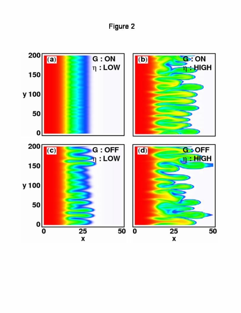
B. Effect of collisionality and X-point geometry on turbulence

In this section, we compare four simulations chosen to contrast the effects of

collisionality (HIGH or LOW) and X-point geometry (ON or OFF). The parameters of

the simulations are as follows. (All variables and parameters are dimensionless, with

physical units given in Sec. II.) Lx1 = 16π , Ly1 = 64π, with Lx2 = Lx1/f and Ly2 =

Ly1⋅f, where f is the fanning parameter defined in Eq. (2). The numerical grid is 256×256

in both regions, so f = ∆x1/∆x2 = ∆y2/∆y1, the ratios of grid spacings. For the fanned and

sheared cases, “geometry on” (G: ON), displayed in Figs. (2a) and (2b), we take f = ¼

and ξ = 4. For the two cases without fanning and shear, “geometry off” (G: OFF), in

11

Figs. (2c) and (2d), f = 1 and ξ = 0. (We discuss the numerical implementation of the

field-line mapping between the two regions in Appendix B of this paper.) In all cases, β

= σ23 = 10-3. For low resistivity cases (η: LOW), Figs. (2a) and (2c), we use η ≡ 1/σ12 =

104, and η = 105 for the high resistivity cases (η: HIGH), Figs. (2b) and (2d). The

diffusion coefficients of vorticity and density are µ1,2 = D1,2 = 10-2 in all cases. The OM

initial conditions are n1(x,y) = n0(x) + δn(x,y) and Φ1(x,y) = 0, where n0(x) is the

reference profile given in Sec. II, and we take x0 = Lx1/4, ∆x0 = 10 ∆x1 , nF = 0.01 and nE

= 1.0, effectively normalizing density to the physical value at the edge boundary (x = 0).

δn is a spatially random perturbation between 0 and 0.01. The XP initial conditions are

field-line copies of those in the OM, but with a different random sequence for δn.

The assumption (used here for simplicity) of constant σ23 has important

consequences for the simulations. Other work on turbulent momentum transport18 has

shown that the sheath provides a momentum sink that damps sheared flow, and that a

sheared flow layer in the edge plasma modifies the blob creation process. The interplay

of sheared flows (which can stabilize the turbulence in some regimes) and density profile

modifications due to blob ejection is a complicated and fascinating subject which we

shall defer to future publications, focusing here instead on the effects of magnetic

geometry and collisionality. Suffice it to say that we expect that the radial streamers seen

in the simulations described here would have been more blob-like if we had set σ23 = 0

inside the edge plasma near x = x0.

In Figure (2) we present snapshots of the density in the OM for the four

simulations. The four snapshots in Fig. (2) are taken at a time, t = 1200, much larger than

the e-folding times of the fastest growing modes: 50 in (a) and (c), 43 in (b) and (d).19 It

is clear that the profile instability gives birth to streamers or blobs that propagate into the

SOL and that blob radial velocity is significantly greater in the high resistivity cases than

in the low resistivity cases; compare (a) to (b) and (c) to (d). This is consistent with

previous observations, particularly the BOUT simulations8 that inspired the present study,

12

in which transport was found to increase with collisionality. But Fig. (2) also suggests

that magnetic geometry (field-line fanning and shear) retards the development of blobs

from the instability and reduces the radial velocity of blobs in the SOL; compare (a) to (c)

and (b) to (d).

A “bloblet analysis” allows us to isolate those structures which dominate the

turbulent radial flux, i.e., the blob-streamers in Fig. (2). Here and henceforth a blob is, by

definition, a density fluctuation for which there exists a Gaussian function that is a

sufficiently good local approximation in y to the fluctuation. Our analysis and goodness-

of-fit criterion are discussed further in Appendix C.

In Figure (3) we plot Φ2 versus Φ1 for blobs detected at x = 30 in the OM for the

four turbulence simulations. Each dot in the figure represents one blob, and the entire

duration of each simulation is represented [∆t = 20,000 in (a) and 10,000 in (b)–(d)]. Φ1

is measured at the center of the bloblet, and Φ2 is measured at the field-line image point

in the XP. This gives us a measure of electrical connection between the two regions, with

perfect connection corresponding to the identity line. Clearly collisionality disconnects

the two regions: the cases of low resistivity, (a) and (c), are connected compared to those

of high resistivity, (b) and (d).

In each case, the blobs are approximately distributed about a straight line through

the origin, with some dispersion about that line. This is to be expected particularly in the

sheath-connected limit: the parallel current balances the sheath current, the right-hand

side of Eq. (5) is zero, and (ignoring diffusion) Φ2 / Φ1 = (1 + σ23.n2 / σ12)-1 ~ 1 / (1 + Λ).

In this limit, Φ1 and Φ2 are highly correlated, with fluctuations in the XP blob density, n2,

providing dispersion about a line whose slope approaches unity, from below, in the limit

of zero resistivity (σ12 / n2 → ∞) and become less connected (and de-correlated) as the

resistivity increases.

The nonlinear polarization currents couple the potentials across field lines, ∇.Jpol

~ k⊥4, and are responsible for instability (Kelvin-Helmholtz)20 and turbulent mixing

13

(cascading) in the separate regions. Therefore the potentials are expected to be

increasingly uncorrelated as Jpol dominates the current budget in either region. The

magnetic geometry enhances cross-field conductivity in the XP region.8,12 In particular,

the streamers of Fig. (2) have ky12 >> kx1

2 so that σ⊥2 ~ k⊥22 ≅ k⊥1

2 . (ξ2 + 1/f2), implying

σ⊥2 / σ⊥1 ≅ 32 for the cases with magnetic geometry on, Figs. (3a) and (3b). Thus by

amplifying the nonlinear, mixing polarization current in the XP, magnetic geometry de-

correlates Φ1 and Φ2 as seen by comparing Figs. (3b) and (3d).

One way to quantify the collisional disconnection and geometric de-correlation

discussed here is to use the Pearson measure of correlation; taking the inner products of

the datasets we find that δΦ1· δΦ2/ (δΦ1· δΦ1 δΦ2· δΦ2)1/2 = (0.996, 0.867, 0.999, 0.958)

for the blob data in cases (a, b, c, d) of Fig. (3).

Figures (2) and (3) are consistent with the blob “circuit diagram” picture.21

Recall that in the blob model of turbulent transport,15 the poloidal gradient of the density

in Eq. (3) drives dipole charge separation across the blob, and the resulting E×B drift

propels the blob radially outward in the OM. This charge polarization mechanism is

essentially the Rosenbluth-Longmuir mechanism22 for the linear interchange instability,

applied here to the density contours of the blob to obtain the nonlinear transport. To

obtain a complete picture of all the blob parameter regimes, this classic blob model needs

to be viewed dynamically in terms of charge flow (current); the curvature-driven current

in the blob is fixed by the driving force, and the net blob potential responsible for the

E×B motion is proportional to the net resistance in the blob circuit, which depends on the

collisionality and geometry.21

Of the four turbulence simulations, the case of low-η and magnetic geometry on

(a) offers the path of least resistance to current flow, both along field lines and across

field lines in the XP, and produces the slowest blobs. With the geometry off (c), the

resulting drop in cross-field conductivity shifts current loop closure to the sheath; the

resistance is increased, and the blobs speed up. In the high-η cases, (b) and (d), the two

14

regions are relatively disconnected. With the magnetic geometry off (d), the polarization

current in the OM provides the path of least resistance and, because this is the most

resistive such path of all four cases, the fastest blobs are produced. Turning the geometry

on (b) slows down the blobs, again, due to enhanced cross-field conductivity in the XP.

To summarize: magnetic geometry reduces blob velocity, while collisionality increases it.

The density flux, which we examine next, behaves similarly.

In Figure (4a) we plot the poloidally-averaged radial particle flux, ⟨Γ⟩y = ⟨n.vx⟩y,

measured at x = 30 in the OM, as a function of time for the four simulations, and the

probability distribution function (PDF) of Γ for all y and t, at x = 30, in Fig. (4b).

Temporal intermittency is observed in all cases, though in the low-η, geometry-on case

(dash-dotted), the intermittent bursts occur on a much longer time scale than in the other

three cases and are of much smaller amplitude. This data is measured at a point and so

resembles the experimental “probe” data23-26 that measures ion saturation current (Isat) at

a point in the tokamak SOL. As seen in Fig. (4b), the PDFs of flux for all four

simulations are similar, and thus insensitive to collisionality and geometry, when plotted

against flux normalized by standard deviation, σΓ, as are those of the experimental data

(with respect to σIsat) across several machines which differ greatly in their geometry and

underlying physics.24 All PDFs are strongly skewed to positive Γ (Isat) with exponential

tails, consistent with the universal, non-diffusive mechanism (blob dynamics) underlying

the observed transport. The presence of a positive tail and the absence of sensitivity to

detailed parameters in the PDFs are important points of agreement between the two-

region model turbulence simulations and the experimental data. In fact, the PDFs in Fig.

(4b) are nearly identical to the ones measured experimentally in Ref. 24. On the other

hand, such agreement, while necessary, is hardly sufficient to validate the present model.

The (numerically and experimentally) observed insensitivity of the PDFs show that this

statistical measure reveals little about the underlying physical processes.

15

The same charge polarization mechanism that propels positive density

fluctuations radially outward moves density depressions radially inward. In the nonlinear

regime, “holes” move backwards toward the core,27 accounting for the relatively weak

negative flux recorded in Fig. (4b). Holes occur in the wakes of isolated blobs and are

produced in blob-blob interactions. See Figs. (1) and (2).

The poloidally and temporally averaged density profiles in the OM, n(x), are

displayed in Fig. (5a), the logarithmic derivative of these profiles in Fig. (5b), and the

skewness S(x) of the density fluctuations in Fig. (5c) for the four simulations. ( S =

⟨(n(x,y,t)–⟨n⟩ y, t) 3⟩ y, t / σ 3, where σ is the standard deviation of the density fluctuations,

indexed by y and t, at a fixed value of x.) First, we observe in Fig. (5a) that in all four

cases the strong turbulent radial particle flux creates a two-scale density profile with a

nearly-constant density shelf extending into the far SOL as a result of the blob

convection. The magnitude of the far-SOL density in the four simulations is proportional

to the convective particle flux in each case [compare with Fig. (4a)]. As an aside we

mention that a parallel particle loss term was not included in the OM continuity equation,

which restricts validity of the model to cases in which the convective radial transport is

much faster than the parallel sonic flow.

The second important result in Fig. (5) is that the radial location of the maximum

of the logarithmic density gradient, -d(ln n)/dx, for each of the four simulations [Fig.

(5b)] coincides with the location where the skewness S of the density fluctuations

vanishes [Fig. (5c)]. As seen from the density profile in Fig. (5a), this point also marks

the transition between the sharp-gradient (diffusive) and weak-gradient (convective)

turbulent particle transport regions, and thus is correlated with the blob generation zone.

The correlation of blob generation with the maximum logarithmic pressure gradient has

also been observed experimentally using the gas-puff-imaging diagnostic.28,29 These

features lead to a consistent physical picture of blob formation, which we now discuss.

16

Experimental data and simulations indicate that the density blobs arise from the

nonlinear saturation of linear instabilities at the plasma edge. For example, curvature-

driven blobs tend to arise near the maximum of the linear growth rate, or equivalently, of

-d(ln n)/dx for interchange and ballooning modes. We refer to this radial location as the

“birth zone” of the blobs. The small initial positive and negative density perturbations of

the interchange mode grow and eventually disconnect as part of the turbulent saturation

process, forming blobs and holes, respectively. (The exact saturation mechanism is

thought to depend on profile modification, wave-breaking, sheared flow generation and

nonlinear cascades, depending on regime.) At this point the Rosenbluth-Longmuir

charge-polarization mechanism, which was driving the linear instability, causes the

coherent objects to move: the positive-density blobs move outwards and the negative-

density holes move inwards. Since the blobs and holes are emitted intermittently, one

would expect that their creation and propagation should be reflected in the higher

statistical moments, e.g. in the skewness S. As seen in Fig. (5), the statistical analysis of

the turbulent fluctuations in the present simulations supports this picture. In each case, we

find that S(x) changes sign near the point of maximum linear growth rate: S = 0 in the

birth zone (reflecting the equal number of blobs and holes created by the interchange

nature of the underlying instability), S < 0 in the direction of hole propagation (up the

magnetic field and density gradients), and S > 0 in the direction of blob propagation

(down the magnetic field and density gradients). The identification of the blob birth zone

with the location where S = 0 is also supported qualitatively by experimental data on

several machines26, 28, 30, 31 and by previous simulations32 that observe a skewness

profile very similar to the one obtained here.

These observations motivate the following decomposition of the turbulent flux

into components that characterize the blob transport. We take S(xb) = 0 to define the

radial location of blob birth, xb, and measure the blob birth density there, nb = n(xb). We

write the averaged density as n(x) = fp(x).nb, and define the blob packing fraction fp(x),

17

which is related to the blob creation rate as follows. If all blobs have density nb, then fp

measures the mean blob duty cycle (0 < fp < 1): the average blob duration at a fixed point

divided by the mean time between blob arrivals at that point. However, the blobs are

absorbed by diffusion and fragment as they propagate, so that fp more generally provides

a lower bound of the duty cycle. (Previous analyses of turbulence data on a reversed

field pinch33 and NSTX34 used a definition of the packing fraction very similar to the

one used here.) We measure the poloidally and temporally averaged radial flux, )x(Γ =

⟨Γ⟩y,t, from the simulations and define the flux-weighted average blob velocity in the

obvious way: )x(vx = )x(Γ /n(x), or )x(Γ = fp(x).nb. )x(vx .

The average flux, Γ , and its three components ( xv , fp, nb) , measured at x = 30,

are recorded in Table I for the four simulations. (We refer to this as “probe data” for the

simulation because the measurements are made at a point in the SOL and hold no

information about the geometrical properties of the blobs, such as cross section, ay, and

particle transport rate, ay.Γ, that are available from the bloblet analysis described above.)

From Table I, we see that the flux increases by a factor of 30 in going from the most

connected case (a) to the least connected case (d) and that most of this increase is due to

the 6–fold increase in the blob velocity, Γ /n, with a 3–fold increase in the packing

fraction and a relatively modest increase in the birth density nb. In comparing the other

cases we see that this is generally true: much of the change in flux results from changes in

the average blob velocity, with the packing fraction playing a secondary role.

This is an interesting and important result which will require verification or

extension to more general situations where the blob generation rate (or packing fraction)

may be controlled by physics not in the present model, e.g. sheared flows or other

regulation mechanisms which can make the edge gradients marginal. In the present

context of robustly unstable edge plasma, the implication is that the part of the blob flux

that is understood analytically (the velocity scaling) is more important than the part that

18

must be computed by a code (the packing fraction). Ultimately, it will be desirable to

have a general predictive theory of the scaling of the total flux.

The trends observed in the flux-weighted probe velocity are echoed in the blob

data. In Table I we record the average radial velocities of blobs for which the particle

transport rate, ayΓ is positive. A 7-fold increase in blob velocity is observed in going

from case (a) to case (d), compared to the 6-fold increase for the probe data, and again

the intermediate cases are indistinguishable. This agreement between the blob velocities

and flux-weighted probe velocities supports the conclusion that the scaling of the

turbulence is dominated by blob physics.

The cases of intermediate flux, (b) and (c), are fairly indistinguishable with

respect to flux, velocity and packing fraction, consistent with the near-perfect overlap of

their average density profiles in Fig. (5a). Case (b) has higher conductivity across field

lines in the XP, thanks to the magnetic geometry, but relatively low parallel conductivity

due to higher collisionality. Case (c) represents the opposite situation: high parallel

conductivity and low cross-field conductivity. Apparently the respective paths of least

circuit resistance are similarly conducting and interchangeable with respect to blob

dynamics in the two cases.

C. Bloblet analysis

We have also calculated the PDFs of H ≡ ay.Γ, the particle transport rate by an

individual blob. (ay is the poloidal half-width. See Appendix C.) We find that the PDFs

of H are similar to those of particle flux obtained from the probe data. For example, 40%

of the total positive H is found at H > 2.σH, with a similar fraction of the total positive

particle flux at Γ > 2.σΓ from the probe data, consistent with experimental results35 and

other simulations.36 These high-H blobs rarely occur, comprising less than 10% of the

blob population in each simulation. They contribute so much to the total H budget

because their high velocities more than compensate for their infrequent occurrence.

19

We define a mean particle transport rate, fp.nb

.⟨vx⟩.⟨ay⟩, analogous to the mean flux

used in the probe data analysis, where the averages may be restricted to a filtered subset

of the blob collection in each simulation, e.g., H > 0, H > σH, H > 2.σH, etc.37 Consistent

with the flux data, H increases with disconnection for all thresholds, and the increase is

dominated by the increase in radial velocity, as for the probe flux data. Comparing the

most connected, lowest-H case (a) to the most disconnected, highest-H case (d), we

observe a 9-fold increase in H dominated by a 7-fold increase in radial velocity, at the

highest threshold (2.σH). Packing fraction and birth density increase by 60%, whereas

blob width, ⟨ay⟩, decreases by a factor of 2 with disconnection.

In Figure (6a) we plot the average blob radial velocity versus ay for the four

simulations, with vx and ay normalized to v* and a

* respectively. (See Sec. III.) The data

has been filtered by requiring H > 0 of each blob. The average blob collisionality

parameters, ⟨Λ⟩, for the four simulations are listed in the final column of Table I. With

reference to the blob regime diagram [Fig. (1) of Paper I], we find that the most

disconnected, highest-H blobs (high-η, G: OFF) are largely in the resistive ballooning

(RB) regime; a greater fraction are found in the resistive X-point (RX) regime with the

geometry on (high-η, G: ON); and for low-η the blobs are in the connected-sheath and

connected-interchange regimes (Cs, Ci), as expected.

Asymptotic velocity scalings inferred from the blob dispersion relation, c.f. Sec.

III, are indicated by solid lines in Fig. (6a) for the RB and Ci regimes (vx ~ 1/2ya ) and for

the RX and Cs regimes (vx ~ 2ya− ). The blob data clusters loosely about these curves but

does not lie on them, and the largest observed velocities exceed the theoretical upper

bound for circular (i.e. isotropic) blobs of 1vx = for small a . The scalings are based on

strong inequalities (Paper I, Sec. III) imposed on the BDR that are not satisfied by the

data, in general. But perhaps more telling, in some cases, is the assumption of blob

isotropy implicit in the BDR.

20

The blob data analysis is, of course, very sensitive to filtering, indeed to the

definition of a “blob” itself. For example, in Fig. (6b) we plot the velocity versus width

of individual blobs, filtered by requiring that each represent a local maximum in x, as

well as y. These are the roundest blobs in our collection of thousands of blobs in total,

and are arguably closest to satisfying the assumption of blob isotropy, ax = ay. It is clear

that the vast majority of blobs are not local x-maxima; they are (poloidal slices of)

streamers, and they are moving about twice as fast as anticipated for isotropic blobs of

width ay, in the most disconnected (high-η, G: OFF) case. This speed-up is apparently

due to streamer geometry, as we now show.

In the strongly disconnected (RB) limit, the polarization current balances the

curvature-driven current source in the OM. Assuming ∂x ~ 1/ax, ∂y ~ 1/ay and equating

the convective derivative of vorticity to the curvature drive term (~β) in Eq. (3), we find

the velocity scaling 2/12x

2y

2/1yx0xx )/aa1/()a/a(vv += , where 2/1

y0x )a(v β= . For

streamers, an aspect ratio (ax/ay) of 4 increases vx by a factor of approximately 23/2 over

the isotropic case, more consistent with the present simulations.

A recent analysis of gas-puff-imaging data shows that the blobs observed

experimentally in the SOL tend to be isotropic and their radial velocity to be bounded by

1vx = .18,29 As mentioned earlier, simulations not discussed here18 indicate that the

radial streamers tend to be broken up into more isotropic structures when a velocity shear

layer is allowed near x = x0 (by turning off the sheath conductivity there, σ23 = 0). This is

also supported by the simulation results of other groups38 Thus, future extensions of the

bloblet analysis with the two-region model will include the effects of a velocity shear

layer near the edge plasma.

V. Conclusions

Using a unique two-region simulation model, introduced in Paper I of this series

and summarized in Secs. II and III, we have studied turbulent transport by blobs, driven

21

by the pressure gradient instability in the outboard midplane, as a function of electrical

connection with the X-point region of a diverted tokamak.

The model used in paper I was generalized here to include magnetic shear along

the field lines, and was applied to simulate isolated blob propagation in Sec. IV A. It was

shown that magnetic shear induces poloidal velocity in isolated blobs in the low-

collisionality regime.

In the turbulence regime (discussed in Secs. IV B and C), we demonstrated a

number of results using the two-region model simulations:

(1) The particle flux increases with collisionality but is reduced by magnetic

field-line fanning and shear. We argued that this is consistent with the circuit diagram

picture9 underlying blob dynamics. Magnetic geometry dramatically enhances cross-field

conductivity in the X-point region, slowing down the blobs, but it also de-correlates the

electrostatic potential fluctuations in the two regions, as noted previously,8,39 and

supports the proposal to use turbulent transport to spread the divertor heat load without

affecting the core and OM SOL plasmas.40

(2) The PDFs of flux that we measure in the simulations, like the PDFs of probe

saturation current measured in experiments, are insensitive to the details of the plasma

parameters (here, collisionality and magnetic geometry); all the PDFs overlap when

plotted as functions of flux normalized by standard deviation. They are strongly skewed

to positive flux with exponential tails underscoring the non-diffusive, ballistic (blob)

nature of the transport.

(3) We observed that the skewness of the density fluctuations passes through zero

at the radial location where the turbulent profile instability growth rate is maximized, in

each simulation, and we identified this location with the birth zone of the blobs.

Decomposing the flux into the product of birth-zone density, packing fraction and radial

velocity, we showed that increases in flux in all cases, whether due to increased

collisionality or the absence of field line fanning and shear, are affected both by increases

22

in blob velocity, and increases in packing fraction (or equivalently, rate of blob

production) with the former playing a somewhat more important role. A bloblet analysis

of particle transport rate, ayΓ, led to similar conclusions.

(4) The bloblet analysis was used to explore the dependence of the blob velocity

on the poloidal blob width for comparison with theoretical scalings. The data clusters

approximately where expected, with scalings predicted by the BDR best supported in the

sheath-connected regime. The large velocities ( 1vx > ) observed in the disconnected

resistive-ballooning regime were shown to be caused by the elongation of the radial

streamers.

This study clearly demonstrates the value of reduced numerical modeling in

identifying the essential physics underlying edge and SOL transport phenomena. It is

anticipated that straightforward extensions of the model to simulate closed field-line

physics, and to include sheared flow and temperature evolution will yield new physics

results to aid in the interpretation of 3D turbulence simulations and experiments.

Acknowledgments

This work was supported by the U.S. Department of Energy (DOE) under grant

DE-FG02-97ER54392; however, such support does not constitute an endorsement by the

DOE of the views expressed herein. Appendix A: Time-advancing algorithm and boundary conditions

The overall algorithm is split-step, with each term in Eqs. (3) – (7) used to

advance the fields in succession. For example, we advance Eq. (3) as follows. Given the

charge density (negative vorticity), ρ1 ≡ −∇2Φ1, at t = 0, we (a) explicitly update it with

the source term, )0()0()( 111 nta y∂⋅⋅∆+= βρρ , and solve Poisson’s equation for Φ1(a).

Next we (b) advance )(1 aρ (and )0(2ρ ) using the parallel current term with an explicit,

staggered two-step method that may be iterated with a reduced local time step to achieve

23

stability. With ρ1(b) as the initial field, we (c) solve the convection equation,

0111 =∇⋅+∂ ρρ vt , using the velocity at the top of the time loop, v1(0). With this result,

ρ1(c), as initial condition, we (d) solve the diffusion equation, 12111 ρµρ ∇=∂t . This gives

us the vorticity at the end of the time loop, )(1 tt ∆=ρ , where each step, (a) – (d), uses the

time increment ∆t. The other fields are similarly updated, and the loop is repeated, etc.

Convection of all fields, as in (c) above, is by the (bi-directional, “phoenical”)

SHASTA algorithm with two-dimensional flux limiter due to Zalesak.41 In

benchmarking exercises that recovered linear growth rates to our satisfaction, we

confirmed the well-known result that this flux-corrected transport algorithm significantly

reduces the numerical dissipation found in simpler algorithms (e.g., Lax-Wendroff).

Furthermore, the algorithm resolves the formation of steep fronts, and cascading to high

vorticity, without apparently generating spurious (Gibbs) oscillations. Positivity of

density under convection is assured, provided a Courant-like constraint is satisfied,

|v|∆t/∆x < ½, which limits the time step used in the simulations in practice.

The diffusion equation for each field, e.g., step (d) above, is solved by the bi-

directional, implicit Crank-Nicholson algorithm,42 and Poisson’s equation is solved by

Fourier analysis with cyclic reduction (FACR).43

The model equations are solved with continuously periodic boundary conditions

in y. We hold Φ1,2 and ∇2 Φ1,2 equal to zero at the radial (x) boundaries. At the edge

boundary (x = 0), n1 and n2 are held equal to unity, establishing the edge boundary

density at t = 0 as the unit of density. The radial gradient of n1,2 is also held equal to zero

at the edge boundary, so the density flux is zero there.

Elementary out-going boundary conditions at x = Lx, for the convection

algorithm, produced unacceptably large charge fluctuations at that boundary. In an

attempt to cure this, we introduced an artificial out-going flow in a neighborhood of the

boundary. In this boundary layer, the radial velocity used in the convection algorithm is

interpolated between the self-consistent radial velocity (−∂yΦ1,2) and a constant positive

24

“Hoover” velocity, vH (typically ¼ ∆x/∆t), where the interpolation is weighted

increasingly to vH as the boundary is approached, as follows: vx = vH + (–∂yΦ(x,y)

− vH)(Lx−x)2/(Lx/8)2, for ⅞ ≤ x/Lx ≤ 1, in both regions. (vy = ∂xΦ(x,y) everywhere.)

This produces a strong out-going flow in the SOL boundary layer, apparent in Fig. (5a),

and eliminates the problem of large charge fluctuations at the boundary in the present

simulations.

Appendix B: Field line fanning and shear

Field-line fanning distinguishes the representation of spatial gradients on the

Cartesian grids in the two regions and is trivially accommodated. For example, the

Poisson equation solver can be called with different grid point spacings (∆x, ∆y). If it is

called with spacings (∆x1 , ∆y1) in region 1, then it is called with spacings (∆x2 , ∆y2) =

(∆x1/f , ∆y1·f) in region 2. The partial time steps are similarly flexible, e.g., the

convection algorithm is called with grid spacings and velocities (gradients of Φ1,2)

appropriate to the region at hand.

Magnetic field-line shear affects only the parallel current terms (∝ σ12) in Eqs. (3)

and (5), where Φ1 and Φ2 are differenced on the same magnetic field line in their

respective regions, consistent with the field-line mapping, Eq. (2). But the Cartesian grid

labels for a field line are different in the two regions. A field passing through grid point

(i1, j1) in region 1 passes through (i2, j2) in region 2, where i2 = i1 , and j2 = j1 + ξG · (i1 –

1), modulo ny – due to the periodic boundary conditions in y in both regions. [We use

the same grid dimensions (nx, ny) in both regions.] The grid shear, ξG, must be an

integer and so restricts the spatial shear, ξ = ξG·∆y2/∆x1 in Eq. (2), to discrete values on a

given numerical grid. With periodic boundary conditions, the shear maps straight radial

lines in region 1 (y1 = constant) onto a series of parallel slanted lines in region 2, i.e., a

“barber pole” pattern.

25

Appendix C: Bloblet analysis

The one-dimensional “bloblet” basis set consists of Gaussians in the poloidal

variable (y) parameterized by location (y0) and width (ay):

4/,,0]2)(exp[),;( 022

00 yyyyy LayLyyayyayybB ≤≤∆≤≤−−== .

At any given time t, a poloidal slice (nominally at x = 30) through the density in the OM

reveals bumps in y. A bump is judged to be a blob only if it is well-approximated locally

by one of the bloblets. The goodness of the approximation is defined to be the

normalized inner product between the bloblet and the density,

))((/),,( 1110 bbnnbntaygoodness y ⋅⋅⋅= ,

where ∫≡⋅ dyayybtyxnbn y ),;(),,( 011 and ∫≡⋅ dytyxnnn 2111 ),,( , and the integral is

the discrete numerical version: a sum over the poloidal grid. Notice that this measure of

goodness is independent of the amplitudes of n1 and b. Although technically the

Gaussian is not a wavelet, because it does not oscillate and have zero mean in y, its

derivative does satisfy those conditions, so this Gaussian-fitting procedure is closely

related to the continuous wavelet transform method.44

The goodness threshold that we have adopted for all simulations in this paper is

0.9: the set y0, ay, t is added to the blob collection, for a given simulation, only if

goodness ≥ 0.9. We also demand that y0 be a local maximum in y of n1(x,y,t) and that

there be at most one blob at (y0,t): that of the greatest goodness with respect to ay. Once a

blob has been identified, various measurements are taken at (x, y0, t), e.g., vx, vy, n1, Φ1,

Φ2, etc., and the enhanced set, y0, ay, t, vx, vy, n1, Φ1, Φ2, ..., is appended to the blob

structure for subsequent diagnosis.

26

Table I. Results of the four turbulence simulations. From the “probe” data at x = 30:

temporally and poloidally averaged particle flux, Γ , mean radial velocity, Γ / n, and

packing fraction, fp = n / nb. The (dimensionless) density in the blob birth zone, nb, is

defined to be the density at the radial location where the skewness S of the density

fluctuations vanishes. (The unit of density is that at the edge boundary, x = 0, and the unit

of flux is that density times cs.) From the blob data at x = 30: average radial velocity, vx,

divided by v*, and average collisionality parameter, Λ = n1·σ23/σ12, for blobs at x = 30.

The blob data is restricted to blobs of positive particle transport rate (ayΓ ); the probe data

is not restricted.

Simulation Γ Γ / n fp nb ⟨vx⟩/v* ⟨Λ⟩ Case Probe Probe Probe Blob Blob (a) 2.5x10-4 4.2x10-3 0.21 0.28 0.14 0.095

G: ON η: LOW (b) 3.0x10-3 1.9x10-2 0.41 0.38 0.50 2.6 G: ON η: HIGH (c) 2.8x10-3 1.8x10-2 0.43 0.37 0.49 0.24 G: OFF η: LOW (d) 7.5x10-3 2.5x10-2 0.65 0.46 0.96 3.9 G: OFF η: HIGH

27

Figure Captions

Fig. 1. (Color online) Isolated blob evolution as seen in the OM: n1(x,y) (grayscale or

color) and Φ1(x,y) (contour lines). (a) The initial condition with no fanning (f = 1) and

no shear (ξ = 0), i.e., no “geometry” (G: OFF). The initial condition in the XP is a field-

line copy of that in the OM. (b) The isolated blob in (a) evolved to t = 200. (c) The

isolated blob initial condition with shear and fanning: ξ = 4 and f = ¼ (G: ON). (d) The

isolated blob in (c) evolved to t = 200. Note that magnetic shear induces poloidal

velocity (vy < 0) in blob propagation.

Fig. 2. (Color online) Snapshots of the density in the OM (n1) at t = 1200, for four

turbulence simulations that differ only with respect to parallel resistivity (η = 1/σ12),

magnetic field line fanning (f ) and shear (ξ), i.e., “geometry” (G), as follows. (a): f = ¼

and ξ = 4 (G: ON), η = 104 (η: LOW). (b): G: ON, η = 105 (η: HIGH). (c): f = 1 and ξ

= 0 (G: OFF), η: LOW. (d): η: HIGH, G: OFF. Parameters common to all simulations

are given in the text. High density is dark (red) at x → 0 and low density is dark again

(blue) as x → 50, on a white background representing the initial, quiescent SOL density.

Fig. 3. (Color online) A measure of the degree of electrical connection between the two

regions based on the bloblet analysis: each point represents one blob recorded at x = 30 in

the OM. Φ1 is measured at the center of the blob, and Φ2 is measured at the magnetic

field line image point in the XP. The identity line corresponds to perfect electrical

connection. The simulations are labeled as in Figure 2 and color coded as in subsequent

figures.

28

Fig. 4. (Color online) Character of the radial particle flux, Γ = nvx, at x = 30 in the OM:

(a) time history of the poloidally-averaged flux ⟨Γ⟩y and (b) probability distribution

function P(Γ) versus Γ, normalized by the standard deviation σΓ. The four simulations

are labeled as in Figure 2: (G:ON, η:LOW): dash-dotted (red); (G:ON, η:HIGH): solid

gray (cyan); (G:OFF, η:LOW): dotted (magenta); (G:OFF, η:HIGH): solid black (blue).

Fig. 5. (Color online) (a) Poloidally and temporally averaged density, n(x), (b) (negative)

logarithmic derivative of n(x) and (c) skewness of density fluctuations, S(x), as functions

of radial location in the OM. The four simulations are labeled as in Figure 4.

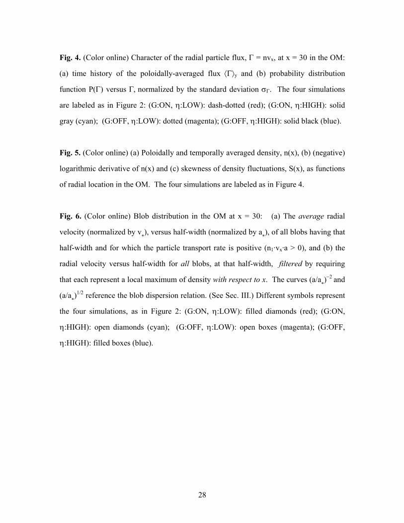
Fig. 6. (Color online) Blob distribution in the OM at x = 30: (a) The average radial

velocity (normalized by v*), versus half-width (normalized by a

*), of all blobs having that

half-width and for which the particle transport rate is positive (n1·vx·a > 0), and (b) the

radial velocity versus half-width for all blobs, at that half-width, filtered by requiring

that each represent a local maximum of density with respect to x. The curves (a/a*)−2 and

(a/a*)1/2 reference the blob dispersion relation. (See Sec. III.) Different symbols represent

the four simulations, as in Figure 2: (G:ON, η:LOW): filled diamonds (red); (G:ON,

η:HIGH): open diamonds (cyan); (G:OFF, η:LOW): open boxes (magenta); (G:OFF,

η:HIGH): filled boxes (blue).

29

References 1 J. R. Myra, D. A. Russell and D. A. D’Ippolito, Phys. Plasmas 13, 112502 (2006).

2 See for example T. C. Hender, B. A. Carreras, W. A. Cooper, J. A. Holmes, P. H. Diamond, and P. L. Similon, Phys. Fluids 27, 1439 (1984), and references therein.

3 J. R. Myra, D. A. D’Ippolito, X. Q. Xu and R. H. Cohen, Phys. Plasmas 7, 2290 (2000); Phys. Plasmas 7, 4622 (2000).

4 B. Scott, Plasma Phys. Control. Fusion 39, 1635 (1997).

5 B. N. Rogers, J. F. Drake, and A. Zeiler, Phys. Rev. Lett. 81, 4396 (1998); B. N. Rogers and J. F. Drake, Phys. Rev. Lett. 79, 229 (1997).

6 X. Q. Xu, W. M. Nevins, T. D. Rognlien, et al., Phys. Plasmas 10, 1773 (2003).

7 B. LaBombard, J. W. Hughes, D. Mossessian, M. Greenwald, B. Lipshultz, J. L. Terry, et al., Nucl. Fusion 45, 1658 (2005).

8 D. A. Russell, D. A. D’Ippolito, J. R. Myra, W. M. Nevins, and X. Q. Xu, Phys. Rev. Lett. 93, 265001 (2004).

9 J.R. Myra and D. A. D’Ippolito, Phys. Plasmas 12, 092511 (2005).

10 D. A. D’Ippolito and J. R. Myra, Phys. Plasmas 13, 062503 (2006).

11 A. V. Nedospasov, Fiz. Plazmy 15, 1139 (1989); [Sov. J. Plasma Phys. 15, 659 (1989)].

12 D. Farina, R. Pozzoli, D. D. Ryutov, Nucl. Fusion 33, 1315 (1993).

13 J. W. Connor and J. B. Taylor, Phys. Fluids 27, 2676 (1984).

14 G. Q. Yu and S. I. Krasheninnikov, Phys. Plasmas 10, 4413 (2003).

15 S. I. Krasheninnikov, Phys. Lett. A, 283, 368 (2001); D. A. D’Ippolito, J. R. Myra, and S. I. Krasheninnikov, Phys. Plasmas 9, 222 (2002).

16 S.J. Zweben, R.J. Maqueda, D.P. Stotler, A. Keesee, J. Boedo, et al., Nucl. Fusion 44 134 (2004); O. Grulke, J. L. Terry, B. LaBombard and S. J. Zweben, Phys. Plasmas 13, 012306 (2006).

17 A. Y. Aydemir, Phys. Plasmas 12, 062503 (2005).

18 J. R. Myra, J. Boedo, B. Coppi, D. A. D’Ippolito, S. I. Krasheninnikov, et al., in Plasma Physics and Controlled Nuclear Fusion Research 2006 (IAEA, Vienna, 2007), paper IAEA-CN-149-TH/P6-21.

19 The growth rate is found by solving the dispersion relation, Eq. (8) in Paper I, extended to include the dissipative terms in the present simulations and evaluating ν(x) and γmhd

2 = −β (ky12 / k⊥1

2) ∂x ln n0(x) at that x for which the (-)logarithmic derivative of n0 is maximized. The initial conditions are all in the RB regime, and therefore the growth rates are independent of fanning and shear.

20 G. Q. Yu and S. I. Krasheninnikov, Phys. Plasmas 10, 4413 (2003).

21 J.R. Myra and D. A. D’Ippolito, Phys. Plasmas 12, 092511 (2005).

30

22 M. N. Rosenbluth and C. L. Longmire, Ann. Phys. 1, 120 (1957).

23 G. Y. Antar, S. I. Krasheninnikov, P. Devynck, R. P. Doerner, E. M. Hollmann, J. A. Boedo, S. C. Luckhardt and R. W. Conn, Phys. Rev. Lett. 87, 065001 (2001).

24 G. Y. Antar, B. Counsell, Y. Yu, B. LaBombard, and P. Devynck, Phys. Plasma 10, 419 (2003).

25 J. A. Boedo, D. Rudakov, R. Moyer, S. Krasheninnikov, D. Whyte, et al. Phys. Plasmas 8, 4826 (2001).

26 D. Rudakov, J. A. Boedo, R. Moyer, S. Krasheninnikov, A. W. Leonard, et al., Plasma Phys. Control. Fusion 44, 717 (2002).

27 S. I. Krasheninnikov, A. Yu, Pigarov, S.A. Galkin, et al., in Proceedings of the 19th IAEA Fusion Energy Conference, Lyon, France, 2002 (IAEA, Vienna, 2003), paper IAEA-CN-94/TH/4-1.

28 J.L. Terry, N.P. Basse, I. Cziegler, M. Greenwald, O. Grulke, B. LaBombard, S.J. Zweben, et al., Nucl. Fusion 45, 1321 (2005).

29 J. R. Myra, D. A. D’Ippolito, D. P. Stotler, S. J. Zweben, B. P. LeBlanc, J.E. Menard, R. J. Maqueda, and J. Boedo, Phys. Plasmas 13, 092509 (2006).

30 J. A. Boedo, D. L. Rudakov, R. A. Moyer, G. R. McKee, R. J. Colchin, et al., Phys. Plasmas 10, 1670 (2003).

31 I. Furno, B. Labit, M. Podesta, A. Fasoli, et al., private communication [2007], (to be submitted to PRL).

32 See the BOUT code results in Fig. 11 of Ref. [30], for example.

33 M. Spolaore, V. Antoni, E. Spada, H. Bergsa ker, R. Cavazzana, J. R. Drake, E. Martines, G. Regnoli, G. Serianni, and N. Vianello, 93, 215003 (2004).

34 M. Agostini, S. Zweben, R. Cavazzana, P. Scarin, G. Serianni, R. J. Maqueda, and D.P. Stotler, private communication [2007], (to be submitted to Phys. Plasmas).

35 J. A. Boedo, D. Rudakov, R. Moyer, S. Krasheninnikov, D. Whyte, et al. Phys. Plasmas 8, 4826 (2001).

36 O. Garcia, V. Naulin, A. H. Nielsen, and J. Juul Rasmussen, Phys. Plasmas 12, 062309 (2005).

37 The normalization of ⟨n⟩ in fp = ⟨n⟩/nb is the total number of blobs, i.e., ⟨n⟩ = Σi`ni / N, where Σi` is restricted to the filtered subset of blobs, and N is the total number of blobs in the unfiltered universe.

38 V. Naulin, private communication [2007].

39 M.V. Umansky, , T.D. Rognlien and X.Q. Xu, J. Nucl. Mater. 337-339, 266 (2005).

40 R.H. Cohen and D. D. Ryutov, Nucl. Fusion 37, 621 (1997); D. D. Ryutov and R. H. Cohen, Contrib. Plasma Phys. 44, 168 (2004).

41 S. T. Zalesak, J. Comp. Phys. 31, 335 (1979), and references therein.

42 W. H. Press, S. A. Teukolsky, W. T. Vetterling and B. P. Flannery, Numerical Recipes in Fortran 77: The Art of Scientific Computing, 2nd ed., p840 (1996).

31

43 P. N. Swarztrauber, SIAM Review 19(3), 490 (1977).

44 M. Farge, Annu. Rev. Fluid Mech. 24, 395 (1992).