Digital Object Identifier (DOI) 10.1007/s10107-005-0622-3

Math. Program., Ser. B 104, 407–435 (2005)

J.E. Harrington · B.F. Hobbs · J.S. Pang ·A. Liu · G. Roch

Collusive game solutions via optimization

It is with great honor that we dedicate this paper to Professor Terry Rockafellar on the occasion of his 70thbirthday. Our work provides another example showing how Terry’s fundamental contributions to convex andvariational analysis have impacted the computational solution of applied game problems.

Received: February 14, 2004 / Accepted: February 16, 2005Published online: July 14, 2005 – © Springer-Verlag 2005

Abstract. A Nash-based collusive game among a finite set of players is one in which the players coordinate inorder for each to gain higher payoffs than those prescribed by the Nash equilibrium solution. In this paper, westudy the optimization problem of such a collusive game in which the players collectively maximize the Nashbargaining objective subject to a set of incentive compatibility constraints. We present a smooth reformulationof this optimization problem in terms of a nonlinear complementarity problem. We establish the convexity ofthe optimization problem in the case where each player’s strategy set is unidimensional. In the multivariatecase, we propose upper and lower bounding procedures for the collusive optimization problem and establishconvergence properties of these procedures. Computational results with these procedures for solving sometest problems are reported.

1. Introduction

In industries characterized by repeated interaction, tacit collusion among producerscan emerge that enables price to drift above single-period Nash equilibrium levels. Anexample of such an industry is the restructured electric power generation sector, whereauctions are held hourly or half-hourly in many markets [21]. Empirical evidence fromthe California and England-Wales markets indicate that prices have exceeded single-period Nash prices for some periods of time [19, 23]. Models of tacit collusion can beuseful to understand how changed market design or structure might affect prices in thesecircumstances.

J.E. Harrington: Department of Economics, The Johns Hopkins University, Baltimore, Maryland 21218-2682,USA. e-mail: joe.harrington@jhu.edu.

B.F. Hobbs: Department of Geography and Environmental Engineering, The Johns Hopkins University,Baltimore, Maryland 21218-2682, USA. e-mail: bhobbs@jhu.edu.

This author’s research was partially supported by the National Science Foundation under grant ECS-0080577.

J.S. Pang: Department of Mathematical Sciences, Rensselaer Polytechnic Institute, Troy, New York,12180-3590, USA. e-mail: pangj@rpi.edu.

This author’s research was partially supported by the National Science Foundation under grant CCR-0098013.

A. Liu: Department of Applied Mathematics and Statistics, The Johns Hopkins University, Baltimore,Maryland 21218-2682, USA. e-mail: lliu@jhu.edu.

G. Roch: Department of Applied Mathematics and Statistics, The Johns Hopkins University, Baltimore,Maryland 21218-2682, USA. e-mail: grantroch@jhu.edu.

Mathematics Subject Classification (1991): 90C26, 90C33, 90C90, 91A10, 91A20

408 J.E. Harrington et al.

Broadly speaking, there are two general approaches to modeling tacit equilibria. Oneis agent-based simulation, in which autonomous agents learn and evolve strategies thatcan mimic tacit collusion. This approach has been applied, for example, to the analysisof market power in the England-Wales energy generation market [3]. The other approachis dynamic equilibrium models, or “supergames”, of the type which is the main focusof this paper. In general, collusion involves firms coordinating their quantity and pricedecisions for the purpose of generating higher payoffs. In considering the incentives tocollude, it is well known that equilibria for most oligopoly models are Pareto-inefficient;that is, all firms could increase their payoff by jointly modifying their decisions. (Fora general statement about the Pareto-inefficiency of Nash equilibria, see Dubey [6].)This Pareto-inefficiency takes the form that all firms would realize a higher payoff ifthey marginally reduced their quantities. The approach in the economics literature tomodelling collusion is to enrich the game by having firms make decisions repeatedly.Quantities that are not equilibria when firms interact only once can be equilibria in thedynamic setting. Of course, if the quantities are not Nash equilibria for the static game,firms can increase their instantaneous payoff by producing differently. To offset thisshort-run gain, dynamic strategies have firms respond to any such deviation by acting ina manner to reduce a deviating firm’s future payoff. This defines a new set of equilibriumconditions that expands the set of equilibrium quantities as one moves from the staticto the dynamic game. For the purpose of the ensuing discussion, let � denote the set ofequilibrium quantities for the dynamic game.

There is one serious weakness with the movement from the static to the dynamicgame – the loss of uniqueness of equilibrium. Under restrictive but plausible assump-tions, the static Cournot game has a unique Nash equilibrium. In contrast, the dynamicCournot game generally has many quantities consistent with Nash equilibrium. Thisleaves open the issue of selecting an element from �. When firms are symmetric, ithas been common practice in the economics literature to focus on the best symmetricelement of�.However, when firms are asymmetric, such as in their cost and capacities,there is no such focal point. The selection from� should be asymmetric but how exactlyshould it relate to firms’ traits?

In thinking about this problem from the firms’ perspective, they are likely to dis-agree over which element of � to choose; each firm wanting to select the one thatgives it the highest payoff. Firms with lower costs probably prefer lower prices and,given any price, each firms desires a bigger market share. In light of such disagree-ment, it is natural to think of firms bargaining to achieve some resolution. This is thebasis for the selection approach formulated in Harrington [12] which uses the set ofequilibrium quantities to construct a bargaining problem. In the axiomatic bargainingliterature (see, e.g., Osborne and Rubinstein [18]), a bargaining problem is definedby a set of payoff vectors, �, which is the set over which players bargain, and a dis-agreement payoff, d ∈�, which is the payoff vector if they fail to reach an agreement.One then applies a bargaining solution to this problem which, under certain condi-tions, produces a unique solution. Applied to our setting, the approach of Harrington[12] is to specify � to be the payoff vectors induced by quantities in � and d to bethe Nash equilibrium payoff for the static game. If one uses the bargaining solutionof Nash [17], the collusive problem can be represented by the following optimizationproblem:

Collusive game solutions via optimization 409

maxq∈�

∏

f∈F

(πf (q)− πN

f

), (1)

where q is the vector of firms’ quantities, πf (q) is the payoff of firm f , πNf is thestatic Nash equilibrium payoff for firm f , and F is the set of firms. To provide someperspective of the formulation (1), previous work had formulated the selection problemassociated with collusion as a bargaining problem but had specified the choice set to bethe set of feasible quantities, which we will denote X, rather than the set of equilibriumquantities; see, for example, Schmalensee [22]. It is now well known that such an ap-proach is flawed because if the solution fails to lie in � then firms have agreed to anoutcome that they have no intent of implementing. Though it is then well motivated toreplace X with �, we are replacing the (typically) convex set X with a set that may notbe convex. Based on their descriptive appeal, we focus on pure stationary outcomes,which prevent achieving convexification through randomization or other means.

Besides providing a formal motivation, this paper aims at studying the collusiveoptimization problem (1) from a global optimization perspective. Due to the possiblenonconcavity of the objective function and the nonconvexity of constraint set, the statedaim is computationally challenging. Our main contributions consist of a set of supportingresults that provide mathematical insights into the problem, the development of upperand lower bounding procedures for the global solution of (1), and the demonstration ofconvergence properties of these procedures.

The organization of the rest of the paper is as follows. In the next section, we present asummary of the variational inequality (VI) approach to computing noncooperative Nashequilibria. This is followed by two sections in which we define and analyze the feasibleset and objective function, respectively, of (1). In particular, we establish a convexityresult in the univariate case in which the strategy set of each player of the game is a com-pact interval; convexity of the collusive game optimization problem is established in thiscase. In Section 5, we present upper and lower bounding procedures in the multivariatecase and establish some convergence results for these procedures. Finally, in Section 6,we illustrate the univariate and multivariate cases with some numerical results.

2. The VI approach to computing Nash equilibria

We begin with a review of the VI approach to the well-known noncooperative Nash equi-librium problem. For a comprehensive study of finite-dimensional variational inequali-ties, see [7]. The players of this game are labelled by the elements f in a finite index setF (for firms). Player f ’s strategy set is denoted Xf , which is a nonempty, convex, andcompact subset of the Euclidean space �nf for some positive integer nf . Elements ofXf are denoted by qf , which are nf -dimensional vectors. Let

X ≡∏

f∈FXf ⊆ �n, where n ≡

∑

f∈Fnf .

Elements of X are denoted by q, whose components are qf for all f ∈ F . We write

X−f ≡∏

f �=t∈FXt, ∀ f ∈ F,

410 J.E. Harrington et al.

and write q−f to denote an arbitrary element of X−f ; thus q−f is the vector withcomponents qt for all t �= f . Player f ’s payoff function is denoted πf , which is a real-valued function defined on �n; thus the payoff πf (q) to player f depends on the vectorof all players’ strategies. We use the alternative notation πf (qf , q−f ) for πf (q) whenwe want to highlight the dependence of player f ’s payoff on his own strategy qf andhis rivals’ collective strategy q−f . Throughout the paper, we postulate that πf (·, q−f ) isa strictly concave function in the argument qf for each fixed but arbitrary q−f ∈ X−fand πf (qf , ·) is convex in the argument q−f for each fixed but arbitrary qf ∈ Xf .

Parameterized by q−f , player f ’s payoff maximization problem is the optimizationproblem in the primary variable qf :

maximize πf (qf , q−f )

subject to qf ∈ Xf .(2)

A Nash equilibrium is a tuple qN ≡ (qNf : f ∈ F) such that for all f ∈ F , qN

f ∈ Xfand

πf (qN) ≥ πf (qf , q

N−f ), ∀ qf ∈ Xf .

We write πNf ≡ πf (qN) to denote the firms’ Nash payoffs. Define the vector function

F(q) ≡ −(∇qf πf (q) : f ∈ F ), q ∈ X. (3)

For ease of later reference, we summarize in the following result properties of the opti-mization problem (2) and the Nash equilibrium.

Proposition 1. LetXf be a nonempty compact convex subset of �nf ; let πf : �n→ �be continuously differentiable and such that πf (·, q−f ) is strictly concave for everyq−f ∈ X−f . The following statements hold.

(a) For all q−f ∈ X−f , a unique maximizer, denoted q∗f (q−f ), exists, which satisfies

( qf − q∗f (q−f ) )T∇qf πf (q∗f (q−f ), q−f ) ≤ 0, ∀ qf ∈ Xf .

(b) If πf (qf , ·) is convex for every qf ∈ Xf then the optimal value function

π∗f (q−f ) ≡ πf (q∗f (q−f ), q−f )

is convex and continuously differentiable with

∇π∗f (q−f ) ≡ ∇q−f πf (q∗f (q−f ), q−f ).(c) IfXf is polyhedral, then q∗f (q−f ), and thus∇π∗f (q−f ), are piecewise smooth func-

tions of their argument.(d) A Nash equilibrium qN exists; moreover qN satisfies

F(qN)T ( q − qN ) ≥ 0, ∀ q ∈ X.(e) IfF(q) is a strictly monotone function onX, then the Nash equilibrium qN is unique.

Collusive game solutions via optimization 411

Proof. The existence, uniqueness, and variational characterization of q∗f (q−f ) are stan-dard results in convex programming. The convexity and continuous differentiability ofthe value function π∗f (q−f ) are immediate consequences of the well-known Danskin’sTheorem [4]. The assertion about the piecewise smoothness of q∗f (q−f ) and ∇π∗f (q−f )follows from sensitivity results of parametric nonlinear programs/variational inequali-ties; see [2, 7, 20]. Finally, the assertions about the Nash equilibrium are well-knownresults; see e.g. [7]. �

In the rest of this paper, we assume that the Nash equilibrium qN is unique; seeProposition 2 where this assumption is used.

2.1. The firms’ payoff functions

For the most part in this paper, we are interested in a Cournot oligopoly problem inwhich the payoff function πf (q) is of the following form:

πf (q) ≡ p(Q)T qf − cf (qf ), (4)

where p(Q) is the market inverse demand (vector) function, with

Q ≡∑

f∈Fqf

being the industry production, i.e., total production by all firms (i.e., players), and cf (qf )is firm f ’s production cost function. We write Q−f ≡ Q− qf for the total productionby firm f ’s rivals. Associated with the Nash equilibrium qN, we write QN and QN

−ffor the industry production and the industry less firm f ’s production, respectively. Theform of the payoff function (4) implies that nf is a constant N for all firms. This isnot a restrictive assumption. Indeed, suppose that each firm has nf plants, with nf notnecessarily equal. Then define N = max

f∈Fnf . We can add N − nf additional plants to

firm f’s collection of plants, each with zero capacity. This minor adjustment will not alterthe most difficult technical challenge of the problem (1), which is its global optimalityand the main concern of our work.

Both functions p(Q) and cf (qf ) in (4) are assumed to be continuously differen-tiable, and additionally, cf is assumed to be convex and nonnegative. The algorithmictreatment in this paper pertains to the further special case where p(Q) is a separableaffine function:

p(Q) ≡ α − Diag(β)Q, (5)

where α and β are positive vectors and Diag(β) is the diagonal matrix whose diago-nal entries are the components of β. For the most part, the cost function cf (qf ) is notrequired to be linear, except in Subsection 5.2 and in the computational tests. With aseparable affine p(Q) as above, it is easy to see that the vector function F(q) in (3)is strictly monotone with a positive definite Jacobian matrix; consequently, the Nashequilibrium qN is naturally unique in a Cournot oligopoly problem.

412 J.E. Harrington et al.

When dealing with the payoff function (4), we employ the following notation:q∗f (Q−f ) for q∗f (q−f ),π

∗f (Q−f ) forπ∗f (q−f ), andπf (qf ,Q−f ) forπf (q); this change

of notation is more descriptive because player f ’s optimal response and his payoff inthis case depend on his rivals’ strategies only through the cumulative output Q−f andnot directly through the individual quantities q−f .

3. The family of collusive sets

This section introduces the family of collusive sets�δ for δ ∈ [0, 1]. We begin by moti-vating these sets using an infinitely repeated extension of the basic Nash game. Someproperties of elements of �δ are then derived. We conclude the section by defining the“Pareto improvement” strategies, which are central to the Nash bargaining optimizationproblem to be formulated and discussed in the next section.

3.1. Motivation

Although noncooperative Nash equilibria involve each firm individually maximizing itspayoff, it is generally not true that firms are collectively maximizing some objectivesuch as the sum of their payoffs. As mentioned in the Introduction, Nash equilibria aregenerally not Pareto-efficient. In many formulations of the Cournot game, this Pareto-inefficiency takes the form that all firms would have a higher payoff if they all marginallyreduced their quantities. It is the possibility that all firms could benefit from coordinationof their quantity choices that provides the basis for observed episodes of collusion inactual markets. As such coordination does not emerge as equilibrium behavior in a stan-dard Cournot game, generation of such behavior requires either forsaking the assumptionof equilibrium or altering the specification of the game. In the economics literature [10],it is typical to maintain equilibrium as a description of firm behavior and instead modifythe game in the direction of greater descriptive realism. In particular, let us now assumethat firms choose quantities repeatedly rather than only once.

The infinitely repeated extension of our game has firms choose quantities and realizepayoffs in each of an infinite number of periods. (What is critical for the ensuing analysisis not that there is an infinite number of periods but rather that there is no upper boundon the number of periods. All results could be derived assuming that the number ofperiods is stochastic as long as, in all periods, a firm assigns positive probability to therebeing at least one more period. For a discussion of repeated games, see Fudenberg andTirole [10].) In defining the strategy space of the infinitely repeated extension, assumethat a firm in period t knows the quantities selected over the previous t − 1 periods sothat its strategy can condition on that information. A strategy for firm f in the infinitely

repeated extension is then an infinite sequence of functions, ρf ≡{ρtf

}∞t=1

, where

ρtf : Xt−1 → Xf and Xt−1 represents the space of period t histories. The strategyset of a firm is the space of all infinite sequences of such functions. Let ρ denote thevector of firms’ strategies and qt−1 ∈ Xt−1 represent a period t history. A firm’s payofffunction for the infinitely repeated extension is assumed to be the sum of discountedsingle-period payoffs,

Collusive game solutions via optimization 413

∞∑

t=1

δ t−1 πf

(ρt

(qt−1

)),

where qt−1 is defined recursively by ρ; that is, it is the sequence of quantity vectorsinduced by firms’strategies. The scalar δ ∈ [0, 1] is a firm’s discount factor and measureshow a firm values a single-period payoff in the next period compared to one in the currentperiod. The weight given to a future single-period payoff declines geometrically in thenumber of periods. Since δ ≤ 1 then current single-period payoffs are valued at least asmuch as those in the future. Also note that as δ declines, less weight is given to futuresingle-period payoffs and when δ = 0 firms care only about their current single-periodpayoff.

Even if there is a unique Nash equilibrium for the single-period game, it is wellknown that the set of Nash equilibria for its infinitely repeated extension can be large. Itis assured of being nonempty since it includes the infinite repetition of the Nash equilib-rium for the single-period game: firm f produces qNf in every period for all f (so thatthere is no conditioning on the history). More interesting is to consider Nash equilibriathat result in quantity vectors distinct from qN and, in particular, generate higher payoffs.This returns us to the issue of collusion which in the context of the infinitely repeatedextension means an equilibrium that yields a higher average payoff than πNf , for all f .(The central result in the theory of repeated games is the Folk Theorem. Define vf as firmf ’s minimax payoff in the single-period game. If πf > vf ∀f and ∃q ∈ X such thatπf (q) = πf then there exists a Nash equilibrium for the infinitely repeated extensionsuch that firm f ’s average single-period payoff is πf ∀f, when δ is sufficiently closeto one. Details can be found in Fudenberg and Tirole (1991).) Arguably the simpleststrategy achieving that objective is the grim trigger strategy [9]. It is defined as follows:for all f ∈ F ,

ρ1f = qf

ρtf ={qf if qτ = q ∀ τ ∈ {1, 2, . . . , t − 1, }qNf otherwise;

}∀ t ∈ {2, 3, . . . } , (6)

where q ∈ X and is to be interpreted as the collusive quantity vector. This strategy saysthat firm f chooses qf in period 1. In any future period, it chooses qf if all past quantityvectors have been q. Given each of the other firms deploys (6), the payoff to firm f

from doing so is πf (q)/(1 − δ) as this strategy profile results in it receiving profit ofπf (q) in every period. For (6) to be a Nash equilibrium, πf (q)/(1− δ)must be at leastas great as that earned from using any other strategy. Another strategy yields a differentpayoff for firm f only if it entails firm f producing a quantity different from qf in someperiod. Without loss of generality, consider a strategy that does so in the first period.Note that the future payoff is πNf /(1− δ) regardless of what firm f produces as long asit is different from qf . This follows from each of the other firms using (6) and that thebest response of firm f is to produce qNf . A necessary and sufficient condition for the

414 J.E. Harrington et al.

strategy (6) to be a Nash equilibrium is then: for all f ∈ F ,

πf (q)

1− δ ≥ πf (q′f , q−f )+ δ

πNf

1− δ ∀ q ′f �= qf

⇔ πf (q)

1− δ ≥ π∗f (q−f )+ δπNf

1− δ⇔ πf (q) ≥ ( 1− δ ) π∗f (q−f )+ δ πNf .

In the repeated game literature, this condition is called an incentive compatibility con-straint. It simply states that unilateral deviation from a collusive solution (“cheating”)should not be more profitable for any firm than continued collusion.

We then define the set of stationary quantity vectors supportable by Nash equilibriato be

�δ = { q ∈ X : πf (q) ≥ ( 1− δ ) π∗f (q−f )+ δ πNf , ∀ f ∈ F }.

The logic behind�δ possibly containing quantity vectors different from qN is as follows.If q �= qN then, by instead choosing q∗f (q−f ), a firm can raise its current single-periodpayoff. Counterbalancing this temptation is the reaction of the other firms’ future quan-tities to such a departure. As long as the inequality in �δ holds, i.e.,

πf (q) ≥ ( 1− δ ) π∗f (q−f )+ δ πNf , (7)

then other firms’ future response sufficiently depresses firm f ’s future payoffs that itdominates the gain in its current single-period payoff. To better illustrate this situation,consider the case where the firms’ quantity vectors are scalars. In this case, under theassumption that firm f ’s single-period payoff function is decreasing in q−f (which isstandard in the literature and will be substantiated in a Cournot oligopoly model; cf. theproof of Proposition 4), satisfaction of (7) then requires that q−f < qN−f so that firm f isdeterred from producing q∗f (q−f ) by the threat that other firms will raise their quantities

from q−f to qN−f in future periods.In general, there are a number of technical questions associated with the set�δ , such

as its nonemptiness, relations between its elements q and the Nash strategy qN, relationsbetween the associated payoffs πf (q) and the Nash payoffs πN

f , and the dependence onδ. The following simple result addresses these questions.

Proposition 2. Let δ ∈ [0, 1] be arbitrary. Assume that the Nash equilibrium qN isunique. For all q ∈ �δ , it holds that

(a) π∗f (q−f )− πNf ≥ πf (q)− πN

f ≥ (1− δ)(π∗f (q−f )− πNf ) ≥ 0;

(b) πf (q) > (1− δ)π∗f (q−f )+ δπNf ⇒ πf (q) > πN

f ;(c) except for δ = 1,

π∗f (q−f ) > πNf ⇒ πf (q) > πN

f .

Moreover, �0 = { qN } and

�1 ={q ≡ ( qf ) ∈ X : πf (qf , q−f ) ≥ πN

f , ∀ f ∈ F}.

Finally, for all 0 ≤ δ1 ≤ δ2 ≤ 1, �δ1 ⊆ �δ2 .

Collusive game solutions via optimization 415

Proof. We first note that the two explicit expressions for �0 and �1 are obvious; theformer is due to the uniqueness of the Nash equilibrium. The first two inequalities in (a)require no proof. For the third inequality, note that

δ ( πf (q)− πNf ) ≥ ( 1− δ ) ( π∗f (q−f )− πf (q) ) ≥ 0.

Hence (πf (q)−πNf ) ≥ 0 if δ > 0. The same must also hold for δ = 0. Hence (a) holds,

from which (b) follows readily, and so does (c).To prove the last assertion of the proposition, let δ1 and δ2 be as given. Let q ∈ �δ1 .

We have

πf (qf ,Q−f ) ≥ π∗f (Q−f )+ δ1 ( πNf − π∗f (Q−f ) )

≥ π∗f (Q−f )+ δ2 ( πNf − π∗f (Q−f ) ),

where the second inequality is by the fact that πNf ≤ π∗f (Q−f ). Thus q ∈ �δ2 . �

The above result shows that the family of collusive sets {�δ : δ ∈ [0, 1]} is expand-ing from the singleton�0, which consists of the single element of the Nash equilibriumsolution qN, to the set�1, which consists of all admissible productions q ∈ X for whicheach firm’s payoff πf (q) is not lower than the Nash payoff πN

f .

3.2. Pareto improvements

A basic motivation in considering collusive strategies is to allow firms to earn higherpayoffs than their respective Nash payoffs. Mathematically, this raises the question ofwhether there exist q ∈ �δ such that πf (q) > πN

f for all f ∈ F . We call such a quantityvector q a Pareto improvement. Due to the fundamental role of this question in the notionof collusion, we give a sufficient condition for a positive answer to the question, basedon the familiar concept of feasible ascent in optimization.

Proposition 3. If there exists q ∈ X such that

∇ψδ,f (qN)T ( q − qN ) > 0, ∀ f ∈ F, (8)

where ψδ,f (q) ≡ πf (q)− (1− δ)π∗f (q−f ), then a Pareto improvement exists.

Proof. It is easy to see that, for q satisfying (8), the vector q(τ) ≡ qN + τ(q − qN) is aPareto improvement for all τ > 0 sufficiently small . Indeed, for such a τ , we have

ψδ,f (q(τ )) > ψδ,f (qN) = δ πN

f

for all f ∈ F . By part (b) of Proposition 2, it follows that πf (q(τ)) > πNf . �

It is interesting to specialize (8) to the payoff function (4). Noting that

∇qt πf (q) ={p(Q)+ Jp(Q)T qf − ∇cf (qf ) if t = fJp(Q)T qf if t �= f ,

416 J.E. Harrington et al.

where Jp(Q) denotes the Jacobian matrix of p(Q), we deduce

∇ψf (qN)T qN = p(QN)T qNf + ( qN

f )T Jp(QN)QN − ∇cf (qN

f )T qN

f .

We also have, for all t �= f ,

∇qt π∗f (qN−f ) = Jp(QN)T qN

f ,

which yields

∇π∗f (qN−f )

T qN−f = ( qN

f )T Jp(QN)QN

−f .

Based on the above expressions, we easily obtain the following corollary of Propo-sition 3, which provides a sufficient condition under which every player can increasehis/her individual payoff above the Nash payoff by simply scaling the Nash equilibriumsolution qN by a factor 1− τ for τ > 0 sufficiently small,

Corollary 1. Let cf (qf ) be a convex function satisfying cf (0) = 0. Assume that cf (qf )and p(Q) are continuously differentiable. If 0 ∈ Xf and

δ (−qNf )

T Jp(QN)QN−f > πN

f + ( qNf )

T Jp(QN)qNf , ∀ f ∈ F,

then a Pareto improvement exists for the Cournot payoff function (4). In fact, (1− τ)qN

is a Pareto improvement for all τ > 0 sufficiently small.

Proof. Continuing the above derivation, we have

∇ψδ,f (qN)T qN

= πNf +cf (qN

f )−∇cf (qNf )T qN

f +(qNf )T Jp(QN)QN − (1− δ)(qN

f )T Jp(QN)QN

−f≤ πN

f + δ(qNf )T Jp(QN)QN

−f + (qNf )T Jp(QN)qN

f < 0,

where the first inequality follows from the convexity of cf and the fact that cf (0) = 0,and the second inequality is by assumption. Consequently, (8) holds with q = 0. Thelast assertion of the corollary is then obvious. �

In general, the existence of a vector q satisfying the ascent condition (8) can bechecked by solving the following convex optimization problem in the variable (q, τ ):

maximize τ

subject to ∇ψδ,f (qN)T ( q − qN ) ≥ τ, ∀ f ∈ Fand q ∈ X.

(9)

Clearly, there exists no vector q ∈ X satisfying (8) if and only if the maximum objectivevalue of the above optimization problem is zero. If each firm f ’s production set Xf ispolyhedral, then (9) is a linear program. In the rest of the paper, we assume that a Paretoimprovement exists.

Collusive game solutions via optimization 417

4. The collusive optimization problem

In considering the problem of collusion, one can think of firms facing two subproblems.First, firms must identify quantity vectors that are sustainable in the sense that if theyagree to produce in a certain manner then it is in the best interests of each firm to doso; in other words, they are equilibria. Second, having identified the set of sustainablequantity vectors, firms must select a particular vector from that set. This is the approachoutlined and implemented in Harrington [12]. The previous section addressed the firstsubproblem by characterizing the set of quantity vectors supportable by a class of Nashequilibria for the infinitely repeated extension. In this section, we take on the secondsubproblem—selecting an element from �δ . When firms are symmetric, it has beencommon practice to focus on the best symmetric element of �δ.When firms are asym-metric, it seems natural that the selection should be asymmetric. For example, firmswith more capacity (as reflected in the upper bound to Xf ) or lower cost should havehigher quantities. Such can be argued from a variety of perspectives; for example, thesingle-period Nash equilibrium has firms with lower cost producing at a higher rate sothe collusive solution should also retain that property. Of course, firms will disagree overhow they rank various payoff vectors. This second subproblem inherently involves bar-gaining among the firms–as they try to resolve their differences–which makes it naturalto use a bargaining solution as a selection device.

In the axiomatic bargaining literature (e.g. [18]), a bargaining problem is defined bya set of payoff vectors, �, which is the set over which players bargain, and a disagree-ment payoff, d ∈ �, which is the payoff vector if they fail to reach an agreement. Inour setting, � = {π (q) : q ∈ �δ} and d = πN. For any (�, d) , a bargaining solutionassigns a subset of � (preferably a singleton). The axiomatic approach to the bargainingproblem is to put forth a set of axioms, which are interpreted to be desirable propertiesfor a bargaining solution to have, and to characterize the solution that satisfies thoseaxioms. This approach was originally laid out in Nash [17] and the Nash bargainingsolution remains the most widely-accepted bargaining solution. In our setting, the Nashbargaining solution solves the following objective which we will refer to as the Nashbargaining objective (NBO):1

θ(q) ≡∏

f∈F

(πf (q)− πN

f

), q ∈ �δ.

1 The Nash bargaining solution is typically formulated in terms of the selection of a payoff vector:

maxπ∈{π(q):q∈�δ }

�f∈F ( πf − πNf ).

The difficulty with this problem is that deriving the choice set is a challenging computational task. Given thatour interest ultimately lies with what firms do rather than what they earn, we have instead formulated theproblem as the selection of a quantity vector:

maxq∈�δ

�f∈F ( πf (q)− πNf ).

Also, Nash originally assumed that � is convex; a property that need not hold for {π (q) : q ∈ �δ}. However,Kaneko (1980) has shown that Nash’s result holds as long as � is compact which is true in our case. Also seeHerrero (1989).

418 J.E. Harrington et al.

The (δ)-collusive game solution is a vector that maximizes θ(q) on the set �δ; thus thecollusive game problem can be stated as the following optimization problem:

maximize log θ(q)

subject to q ∈ �δ.(10)

The logarithmic objective function is well defined and extended-valued (i.e., possiblyequal to−∞) on the feasible set (e.g., when q = qN), and is finite-valued on the subset ofPareto improvements. Clearly, only the latter vectors are of interest in the solution of (10).

In addition to the extended-valued feature of the objective function, there are severalcomputational challenges associated with (10). First and foremost is the nonconvexityof this problem in general (see the next section for more discussion). Another challenge,which endangers the superlinear convergence of computational methods for solving theproblem and complicates sensitivity analysis under data perturbations, is the fact that theonce but not twice differentiable implicitly defined value function π∗f (q−f ) is present inthe constraint set�δ . Fortunately, it is not difficult to derive an equivalent formulation ofthe Karush-Kuhn-Tucker (KKT) system of (10) as a mixed nonlinear complementarityproblem (NCP) that involves only the input functions; in particular, the resulting NCPformulation circumvents the need to evaluate the value function during computations,which is not a trivial task in realistic applications.

To derive the equivalent NCP formulation, we assume that each set Xf is finitelyrepresented:

Xf ≡ { qf ∈ �nf : gf (qf ) ≤ 0 }, (11)

where gf : �nf → �mf is twice continuously differentiable and each component func-tion gf i for i = 1, . . . , mf is convex. In what follows, we present the KKT system of(10) without regards to prerequisite constraint qualifications (CQs); these will be for-mally stated when we analyze the optimization problem rigorously. (A word of caution:while the setXf is polyhedral in many applications, the profit function πf (q) is alwaysnonlinear, thereby rendering the feasible set �δ non-polyhedral in all cases.) The KKTsystem is as follows: for all f ∈ F ,

0 = −∑

t∈F

∇qf πt (q)πt (q)− πN

t

+mf∑

i=1

λf i ∇gf i(qf )− µf ∇qf πf (q)

+∑

f �=t∈Fµt

[−∇qf πt (q)+ ( 1− δ )∇qf πt (q∗t (q−t ), q−t )]

0 ≤ λf ⊥ gf (qf ) ≤ 0

0 ≤ µf ⊥ πf (q)− ( 1− δ ) π∗f (q−f )− δ πNf ≥ 0,

where λf ∈ �mf and µf ∈ � are the KKT multipliers of the constraints defining�δ . Inorder to eliminate the implicit q∗f (q−f ) and π∗f (q−f ), we recall from Proposition 1 thevariational characterization of the former vector, which we can state in terms of anothercomplementarity system. Letting q̃f ≡ q∗f (q−f ), we can write the KKT system for firm

Collusive game solutions via optimization 419

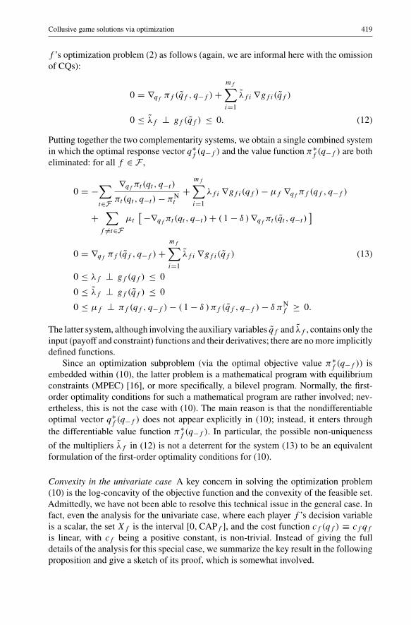
f ’s optimization problem (2) as follows (again, we are informal here with the omissionof CQs):

0 = ∇qf πf (q̃f , q−f )+mf∑

i=1

λ̃f i ∇gf i(q̃f )

0 ≤ λ̃f ⊥ gf (q̃f ) ≤ 0. (12)

Putting together the two complementarity systems, we obtain a single combined systemin which the optimal response vector q∗f (q−f ) and the value function π∗f (q−f ) are botheliminated: for all f ∈ F ,

0 = −∑

t∈F

∇qf πt (qt , q−t )πt (qt , q−t )− πN

t

+mf∑

i=1

λf i ∇gf i(qf )− µf ∇qf πf (qf , q−f )

+∑

f �=t∈Fµt

[−∇qf πt (qt , q−t )+ ( 1− δ )∇qf πt (q̃t , q−t )]

0 = ∇qf πf (q̃f , q−f )+mf∑

i=1

λ̃f i ∇gf i(q̃f ) (13)

0 ≤ λf ⊥ gf (qf ) ≤ 0

0 ≤ λ̃f ⊥ gf (q̃f ) ≤ 0

0 ≤ µf ⊥ πf (qf , q−f )− ( 1− δ ) πf (q̃f , q−f )− δ πNf ≥ 0.

The latter system, although involving the auxiliary variables q̃f and λ̃f , contains only theinput (payoff and constraint) functions and their derivatives; there are no more implicitlydefined functions.

Since an optimization subproblem (via the optimal objective value π∗f (q−f )) isembedded within (10), the latter problem is a mathematical program with equilibriumconstraints (MPEC) [16], or more specifically, a bilevel program. Normally, the first-order optimality conditions for such a mathematical program are rather involved; nev-ertheless, this is not the case with (10). The main reason is that the nondifferentiableoptimal vector q∗f (q−f ) does not appear explicitly in (10); instead, it enters throughthe differentiable value function π∗f (q−f ). In particular, the possible non-uniqueness

of the multipliers λ̃f in (12) is not a deterrent for the system (13) to be an equivalentformulation of the first-order optimality conditions for (10).

Convexity in the univariate case A key concern in solving the optimization problem(10) is the log-concavity of the objective function and the convexity of the feasible set.Admittedly, we have not been able to resolve this technical issue in the general case. Infact, even the analysis for the univariate case, where each player f ’s decision variableis a scalar, the set Xf is the interval [0,CAPf ], and the cost function cf (qf ) ≡ cf qfis linear, with cf being a positive constant, is non-trivial. Instead of giving the fulldetails of the analysis for this special case, we summarize the key result in the followingproposition and give a sketch of its proof, which is somewhat involved.

420 J.E. Harrington et al.

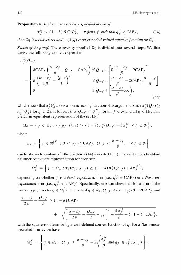
Proposition 4. In the univariate case specified above, if

πNf > ( 1− δ ) β CAP2

f , ∀ firms f such that qNf < CAPf , (14)

then �δ is a convex set and log θ(q) is an extended-valued concave function on �δ .

Sketch of the proof. The convexity proof of �δ is divided into several steps. We firstderive the following explicit expression:

π∗f (Q−f )

=

βCAPf

(α−cfβ−Q−f − CAPf

)if Q−f ∈

[0,α − cfβ− 2CAPf

]

β

(α − cf

2 β− Q−f

2

)2

if Q−f ∈[α − cfβ− 2CAPf ,

α − cfβ

]

0 if Q−f ∈[α − cfβ

,∞),

(15)

which shows thatπ∗f (Q−f ) is a nonincreasing function of its argument. Sinceπ∗f (Qf ) ≥π∗f (Q

Nf ) for q ∈ �δ , it follows that Q−f ≤ QN

−f for all f ∈ F and all q ∈ �δ . Thisyields an equivalent representation of the set �δ:

�δ ={q ∈ �∗ : πf (qf ,Q−f ) ≥ ( 1− δ ) π∗f (Q−f )+ δ πN

f , ∀ f ∈ F},

where

�∗ ≡{q ∈ �|F | : 0 ≤ qf ≤ CAPf ; Q−f ≤ α − cf

β, ∀ f ∈ F

}

can be shown to contain qN (the condition (14) is needed here). The next step is to obtaina further equivalent representation for each set:

�fδ =

{q ∈ �∗ : πf (qf ,Q−f ) ≥ ( 1− δ ) π∗f (Q−f )+ δ πN

f

},

depending on whether f is a Nash-capacitated firm (i.e., qNf = CAPf ) or a Nash-un-

capacitated firm (i.e., qNf < CAPf ). Specifically, one can show that for a firm of the

former type, a vector q ∈ �fδ if and only if q ∈ �∗,Q−f ≤ (α− cf )/β − 2CAPf , and

α − cf2 β

− Q−f2≥ ( 1− δ )CAPf

+√[

α − cf2 β

− Q−f2− qf

]2

+δ πN

f

β− δ ( 1− δ )CAP2

f ,

with the square-root term being a well-defined convex function of q. For a Nash-unca-pacitated firm f , we have

�fδ =

q ∈ �∗ : Q−f ≤ α − cfβ− 2

√πNf

βand qf ∈ Ifδ (Q−f )

,

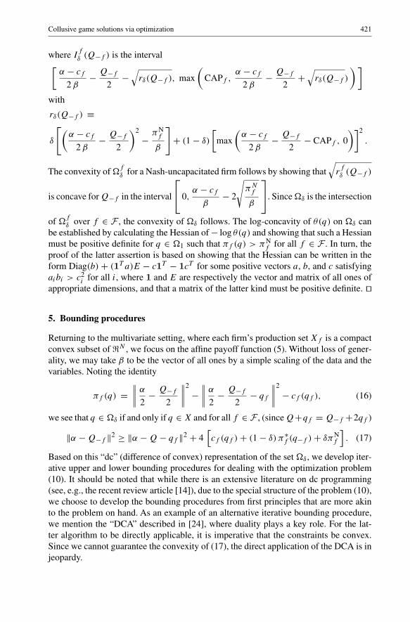
Collusive game solutions via optimization 421

where Ifδ (Q−f ) is the interval[α − cf

2 β− Q−f

2−

√rδ(Q−f ), max

(CAPf ,

α − cf2 β

− Q−f2+

√rδ(Q−f )

)]

with

rδ(Q−f ) ≡

δ

[(α − cf

2 β− Q−f

2

)2

−πNf

β

]+ (1− δ)

[max

(α − cf

2 β− Q−f

2− CAPf , 0

)]2

.

The convexity of�fδ for a Nash-uncapacitated firm follows by showing that√rfδ (Q−f )

is concave forQ−f in the interval

0,α − cfβ− 2

√πNf

β

. Since�δ is the intersection

of �fδ over f ∈ F , the convexity of �δ follows. The log-concavity of θ(q) on �δ canbe established by calculating the Hessian of− log θ(q) and showing that such a Hessianmust be positive definite for q ∈ �1 such that πf (q) > πN

f for all f ∈ F . In turn, theproof of the latter assertion is based on showing that the Hessian can be written in theform Diag(b)+ (1T a)E − c1T − 1cT for some positive vectors a, b, and c satisfyingaibi > c2

i for all i, where 1 and E are respectively the vector and matrix of all ones ofappropriate dimensions, and that a matrix of the latter kind must be positive definite. �

5. Bounding procedures

Returning to the multivariate setting, where each firm’s production set Xf is a compactconvex subset of �N , we focus on the affine payoff function (5). Without loss of gener-ality, we may take β to be the vector of all ones by a simple scaling of the data and thevariables. Noting the identity

πf (q) =∥∥∥∥α

2− Q−f

2

∥∥∥∥2

−∥∥∥∥α

2− Q−f

2− qf

∥∥∥∥2

− cf (qf ), (16)

we see that q ∈ �δ if and only if q ∈ X and for all f ∈ F , (sinceQ+qf = Q−f +2qf )

‖α −Q−f ‖2 ≥ ‖α −Q− qf ‖2 + 4[cf (qf )+ (1− δ) π∗f (q−f )+ δπN

f

]. (17)

Based on this “dc” (difference of convex) representation of the set �δ , we develop iter-ative upper and lower bounding procedures for dealing with the optimization problem(10). It should be noted that while there is an extensive literature on dc programming(see, e.g., the recent review article [14]), due to the special structure of the problem (10),we choose to develop the bounding procedures from first principles that are more akinto the problem on hand. As an example of an alternative iterative bounding procedure,we mention the “DCA” described in [24], where duality plays a key role. For the lat-ter algorithm to be directly applicable, it is imperative that the constraints be convex.Since we cannot guarantee the convexity of (17), the direct application of the DCA is injeopardy.

422 J.E. Harrington et al.

5.1. Upper bounding

The boundedness of the set X induces an upper bound, which we denote κf , on thequantity ‖α − Q−f ‖2 for each f ∈ F . Alternatively, if Xf is contained in the non-negative orthant (which is a typical situation in applications) and if the cost function cfis nonnegative, then the constraint (17) itself trivially induces an upper bound on each‖qf ‖, and thus on ‖α −Q−f ‖2 for all f ∈ F . In what follows, we take the bound κfto be a readily available quantity.

Consider the following set which involves the auxiliary variables ξf for f ∈ F :

�δ ≡ { ( q, ξ ) ∈ X ×�|F | : for all f ∈ F, ξf ≤ κf

ξf ≥ ‖α −Q− qf ‖2 + 4 [ cf (qf )+ ( 1− δ ) π∗f (Q−f )+ δ πNf ]

ξf ≥ ‖α −Q−f ‖2

ξf ≥ ‖α −Q− qf ‖2 + 4 [ cf (qf )+ πNf ] }.

It is clear that �δ is a “relaxation” of �δ in the sense that if q ∈ �δ , then (q, ξ), whereξf ≡ ‖α − Q−f ‖2 for all f , belongs to �δ . Moreover, �δ is clearly a convex set. Torecover the set �δ from �δ , we consider the penalization of the next-to-last inequalityin �δ . Specifically, for each scalar ς > 0, we consider the optimization problem in thevariable (q, ξ):

maximize∑

f∈F

{log

(1

4

[ξf − ‖α −Q− qf ‖2 − 4 ( πN

f + cf (qf ) )])+

ς∑

f∈F

(‖α −Q−f ‖2 − ξf

)

subject to q ∈ X

and ∀ f ∈ F, ξf ≤ κf

ξf ≥ ‖α −Q− qf ‖2 + 4[( 1− δ ) π∗f (Q−f )+ δ πN

f + cf (qf )]

ξf ≥ ‖α −Q− qf ‖2 + 4[πNf + cf (qf )

]

ξf ≥ ‖α −Q−f ‖2.

(18)

By the next-to-last constraint, the logarithmic term in the objective function is a well-defined extended-valued concave function, with value equal to −∞ when equalityholds in the next-to-last constraint; the concavity is easy to verify. The penalty term

ς∑

f∈F

(‖α −Q−f ‖2 − ξf

)in the objective function, together with the final constraint,

is intended to force ξf − ‖α −Q−f ‖2 to zero, hence the log part of the objective func-tion to log θ(q) as ς → ∞. Note that the objective of (18) is a dc function because ofthe term ‖α −Q−f ‖2 The next result summarizes several key properties of the aboveoptimization problem whose maximum objective value we denote ως .

Collusive game solutions via optimization 423

Proposition 5. Let Xf be a nonempty compact convex subset of �N containing theorigin, and let cf be a nonnegative function. The following statements are valid.

(a) For every ς > 0, ως ≥ maxq∈�δ

log θ(q) ≡ ω∞;

(b) ς1 > ς2 > 0 implies ως2 ≥ ως1 , with equality holding if and only if ως2 = ω∞;

(c) limς→∞ως = ω∞.

Proof. The proposition is a type of exact penalty function result for a constrained opti-mization problem. For completeness, we give the details of the proof of parts (b) and(c); part (a) does not require a proof. Let ς1 > ς2 > 0 and let (qν, ξν) denote an optimalsolution of (18) corresponding to ςν for ν = 1, 2. We have

ως2 ≥∑

f∈F

{log

(1

4

[ξ1f − ‖α −Q1 − q1

f ‖2 − 4(πNf + cf (q1

f ))])

+ ς2

∑

f∈F

(‖α −Q1

−f ‖2 − ξ1f

)

≥∑

f∈F

{log

(1

4

[ξ1f − ‖α −Q1 − q1

f ‖2 − 4(πNf + cf (q1

f ))])

+ ς1

∑

f∈F

(‖α −Q1

−f ‖2 − ξ1f

)

= ως1

If ως2 = ως1 , then ‖α −Q1−f ‖2 = ξ1

f for all f ∈ F . Hence q1 belongs to �δ . Conse-quently, ω∞ = ως1 ; and so ως2 = ωδ . The converse is obvious.

Let {ςk} be any sequence of scalars tending to∞ and let (qk, ξk) be a correspondingsequence of optimal solutions of (18). The latter sequence of optimal solutions must bebounded. If (q∞, ξ∞) is any accumulation point of this sequence, then we must have‖α − Q∞−f ‖2 = ξ∞f for all f ∈ F because the sequence of optimal objective values{ωςk } is nonincreasing and bounded below by ω∞, and thus converges. This shows thatq∞ belongs to �δ . �

Ideally, we would like to have a convergent upper bounding procedure that solvesconvex optimization subproblems. In addition to a dc programming approach, one wayto achieve this is via a global optimization method, such as that of convex extension andenveloping [25, 26], possibly embedded within a “branch-and-cut scheme”. Detailedexploration of such a scheme is beyond the scope of this paper and is under developmentin the Ph.D. thesis of Liu.

5.2. Lower bounding

Instead of replacing the left-hand side of (17) by ξf and then penalizing the resultinginequality ξf ≥ ‖α−Q−f ‖2, we use a first-order approximation of the term ‖α−Q−f ‖2for the derivation of lower bounds for the collusive game optimization problem (10).

424 J.E. Harrington et al.

We recall the blanket assumption that a Pareto improvement q0 exists. By definition,q0 belongs to the set �δ and satisfies

π∗f (Q0−f ) > πN

f , ∀ f ∈ F . (19)

If no such vector q0 exists, then the maximization problem (10) is not interesting at allbecause its objective function is identically equal to zero on its feasible set. Noting theequality

‖α −Q−f ‖2 = ‖α −Q0−f ‖2 + 2(Q0

−f − α)T (Q−f −Q0−f )+ ‖Q−f −Q0

−f ‖2,

we see that the set

�δ(q0) ≡ {q ∈ X : ‖α −Q0

−f ‖2 + 2 (Q0−f − α )T (Q−f −Q0

−f )

≥ ‖α −Q− qf ‖2 + 4[ cf (qf )+ ( 1− δ ) π∗f (Q−f )+ δ πNf ] ∀ f }

is a nonempty subset of �δ , nonempty because �δ(q0) contains q0. Moreover, the set�δ(q

0) is convex because the left-hand side of the inequality in �δ(q0) is a linearfunction ofQ−f and the right-hand side is a convex function of (qf ,Q−f ). In essence,�δ(q

0) is obtained by “semi-linearizing” the quadratic function πf (qf ,Q−f ), wherebythe first term in the right-hand side of (16) is linearized atQ0 and the second term is leftintact.

The next result shows that the inequality (19) continues to hold for all elements ofthe set �δ(q0).

Proposition 6. For all q ∈ �δ(q0), π∗f (Q−f ) > πNf for all f ∈ F .

Proof. Let q ∈ �δ(q0). We know that π∗f (Q−f ) ≥ πNf for all f ∈ F . Assume for the

sake of contradiction that π∗f (Q−f ) = πNf for some f ∈ F . We then have

πNf ≥ πf (q) ≥ 1

4‖Q−f −Q0

−f ‖2 + ( 1− δ ) π∗f (Q−f )+ δ πNf ,

which implies Q−f = Q0−f . This contradicts (19). �

Similar to the restricted set �δ(q0), we consider, for a given vector q0 satisfying(19), a lower objective function:

χ(q, q0) ≡∏

f∈F

1

4

[‖α −Q0

−f ‖2 + 2 (Q0−f − α)T (Q−f −Q0

−f )

− ‖α −Q− q ‖2 − 4 ( πNf + cf (qf ) )

],

which has the property that

χ(q, q) = θ(q) ≥ χ(q, q0), ∀ q ∈ �δ(q0). (20)

Collusive game solutions via optimization 425

Taking logarithm of the above lower objective function, we consider the restricted col-lusive optimization problem:

maximize logχ(q, q0)

subject to q ∈ �δ(q0).(21)

Defining

ϕf (q, q0) ≡ 1

4

[‖α −Q0

−f ‖2 + 2(Q0−f − α )T (Q−f −Q0

−f ) −

‖α −Q− q ‖2 − 4( πNf + cf (qf ) )

],

we see that ϕf (·, q0) is a concave in the first variable, and that

χ(q, q0) =∏

f∈Fϕf (q, q

0).

Moreover, ϕf (q0, q0) = πf (q0) − πN

f . The following result summarizes some basicproperties of the optimization problem (20) in the case of linear cost function cf (qf ) ≡cTf qf , where cf is a given vector with components cf i .

Proposition 7. Suppose that Xf is a closed convex subset of �N and that cf i ≥ 0 forall f and i. Let δ ∈ (0, 1) and q0 ∈ �δ satisfying (19) be given. The following threestatements hold.

(a) The function χ(·, q0) is positive and logχ(·, q0) is strictly concave on�δ(q0); thus,(21) is a well-defined concave maximization problem.

(b) Problem (21) has a unique optimal solution, say q1, which satisfies

maxq∈�δ

θ(q) ≥ θ(q1) ≥ maxq∈�δ(q0)

χ(q, q0) ≥ θ(q0). (22)

Moreover, θ(q1) = θ(q0) if and only if q1 = q0.(c) If either [Xf is finitely represented and the Mangasarian-Fromovitz constraint qual-

ification (MFCQ) holds for the set �δ at q0], or [Xf is polyhedral], then θ(q1) =θ(q0) if and only if q0 is a KKT point of the original collusive game optimizationproblem (10).

Proof. For q in �δ(q0), we have

ϕf (q, q0) ≥ ( 1− δ ) ( π∗f (Q−f )− πN

f ).

Therefore, by Proposition 6, it follows that χ(q, q0), being the product of ϕf (q, q0) forall f ∈ F , is positive on �δ(q0). Since

logχ(q, q0) =∑

f∈Flogϕf (q, q

0).

426 J.E. Harrington et al.

it follows that logχ(·, q0) is concave on �δ(q0). To show the strict concavity, let τ ∈(0, 1) and let q and q ′ be two distinct vectors in �δ(q0). For the sake of contradiction,assume that

logχ(τq + (1− τ)q ′, q0) = τ logχ(q, q0)+ ( 1− τ ) logχ(q ′, q0).

Then we must have, for all f ∈ F ,

ϕf (τq + (1− τ)q ′, q0) = τ ϕf (q, q0)+ ( 1− τ ) ϕf (q ′, q0),

or equivalently,

‖α − cf − τ Q− ( 1− τ )Q ′ − τ qf − ( 1− τ ) q ′f ‖2 =

τ ‖α − cf −Q− qf ‖2 + ( 1− τ ) ‖α − cf −Q ′ − q ′f ‖2.

By the strict convexity of the Euclidean norm, it follows that Q + qf = Q ′ + q ′f forall f ∈ F . Summing up these equalities over all f ∈ F yields Q = Q ′, which inturn implies q = q ′. Consequently, the strict concavity of logχ(·, q0) follows. Thisestablishes (a).

The existence and uniqueness of q1 do not require a proof. The first inequality in(22) is obvious because �δ(q0) is a subset of �δ; the second inequality is due to (20);and the third inequality is because �δ(q0) contains q0. If θ(q1) = θ(q0), then we musthave χ(q1, q0) = χ(q0, q0), which shows that q0 is an optimal solution of (21). By theuniqueness of q1, it follows that q1 = q0. Hence (b) holds.

Under the assumptions of part (c), the KKT conditions are necessary optimality con-ditions for (21). Hence, for Xf represented by (11), there exist multipliers λf ∈ �mfand ηf ∈ � such that, for all f ∈ F ,

0 =∑

f �=t∈F

Q1 + q1t −Q0−t

2 ϕt (q1, q0)+Q1 + q1

f − α + ∇cf (q1f )

ϕf (q1, q0)+

mf∑

i=1

λf i ∇gf i(q1f )

+ 4 ηf[q1f +Q1 − α + ∇cf (q1

f )]

+∑

f �=t∈F2 ηt

[( 2 q1

t +Q1−t −Q0

−t )− 4 ( 1− δ ) q∗t (Q1−t )

]

0 ≤ λf ⊥ gf (q1f ) ≤ 0

0 ≤ ηf ⊥ ‖α −Q0−f ‖2 + 2 (Q0

−f − α )T (Q1−f −Q0

−f )

− ‖α −Q1 − q1f ‖2 − 4 [ cf (q

1f )+ ( 1− δ ) π∗f (Q1

−f )+ δ πNf ] ≥ 0.

Collusive game solutions via optimization 427

If θ(q1) = θ(q0), then q1 = q0. Hence the above KKT system reduces to

0 =∑

t∈F

q0t

πt (q0)− πN +Q0 − α + ∇cf (q0

f )

πf (q0)− πN +mf∑

i=1

λf i ∇gf i(q0f )

+ 4 ηf[q0f +Q0 − α + ∇cf (q0

f )]+ 4

∑

f �=t∈Fηt

[q1t − ( 1− δ ) q∗t (Q0

−t )]

0 ≤ λf ⊥ gf (q0f ) ≤ 0

0 ≤ ηf ⊥ πf (q0)− ( 1− δ ) π∗f (Q0

−f )− δ πNf ≥ 0.

With a moment’s verification, the reader can easily see that the above is precisely the KKTsystem of (10) at q0. Conversely, if q0 satisfies the latter KKT system, then q1 ≡ q0 sat-isfies the former KKT system. Since (21) is a concave maximization problem, it followsthat q0 is an optimal solution to it. �

Based on Proposition 7, we propose an iterative algorithm for computing a KKTpoint of (10). The algorithm requires an initial vector q0 ∈ �δ satisfying (19). Such avector can be computed either by first solving the convex program (9) followed by anArmijo-type line search as instructed by Proposition 3, or by employing Corollary 1 ifthe latter is directly applicable.An Iterative Lower Bounding Algorithm.

Step 0 Assume that a vector q0 ∈ �δ satisfying (19) is given. Let k = 0.Step 1 Solve the concave maximization subproblem:

maximize logχ(q, qk)

subject to q ∈ �δ(qk),(23)

and let qk+1 be the unique optimal solution.Step 2 If θ(qk+1)− θ(qk) is less than a prescribed tolerance, stop. Otherwise, let k←

k + 1 and return to Step 1.

Consider an infinite sequence {qk} generated by the algorithm. This sequence iscontained in the bounded set �δ . It therefore has at least one accumulation point. Thesequence of positive scalars {θ(qk)} is strictly increasing and bounded above; it thereforeconverges. Consequently, we have

limk→∞

θ(qk+1) = limk→∞

χ(qk+1, qk).

Since this common limit is bounded below by the positive scalar θ(q0), it follows that

limk→∞

‖Qk+1−f −Qk

−f ‖ = 0, ∀ f ∈ F . (24)

Based on the above limit, we can establish the desired KKT property of an accumulationpoint of the sequence {qk}.

428 J.E. Harrington et al.

Proposition 8. Suppose that Xf is a closed convex, finitely represented subset of �Nand that cf (qf ) = cTf qf , where each constant cf i is nonnegative. Let δ ∈ (0, 1) and

q0 ∈ �δ satisfy (19). The following two statements are valid.

(a) Every accumulation point of the sequence {qk} belongs to �δ .(b) If q∞ is the limit of a convergent subsequence {qk+1 : k ∈ K} for some infinite

subset K such that q∞ satisfies the MFCQ for the set �δ , then q∞ is a KKT pointof (10).

Proof. It suffices to prove (b). Since q∞ belongs to �δ , it follows that πf (q∞) ≥ πNf

for all f ∈ F . Since θ(qk) ≥ θ(q0) > 0 for all k, we must have πf (q∞) > πNf for all

f ∈ F . Since qk+1 satisfies

πf (qk+1)− 1

4‖Qk+1−f −Qk

−f ‖2

= 1

4

[‖α −Qk

−f ‖2 + 2(Qk−f − α)T (Qk+1

−f −Qk−f )− ‖α −Qk+1 − qk+1

f ‖2]

− cf (qk+1f )

≥ ( 1− δ ) π∗f (Qk+1−f )+ δ πN

f ,

and since the MFCQ is invariant under small function perturbations, it follows from (24)that the KKT conditions for (21) must necessarily be satisfied by its optimal solutionqk+1. Therefore, there exist multipliers λk+1

f ∈ �mf and ηk+1f ∈ � such that, for all

f ∈ F ,

0 =∑

f �=t∈F

Qk+1 + qk+1t −Qk−t

2 ϕt (qk+1, qk)+Qk+1 + qk+1

f − α + ∇cf (qk+1f )

ϕf (qk+1, qk)

+mf∑

i=1

λk+1f i ∇gf i(qk+1

f )+ 4 ηk+1f

[qk+1f +Qk+1 − α + ∇cf (qk+1

f )]

+∑

f �=t∈Fηk+1t

[2 ( 2 qk+1

t +Qk+1−t −Qk

−t )− 4 ( 1− δ ) q∗t (Qk+1−t )

]

0 ≤ λk+1f ⊥ gf (q

k+1f ) ≤ 0

0 ≤ ηk+1f ⊥ ‖α −Qk

−f ‖2 + 2 (Qk−f − α )T (Qk+1

−f −Qk−f )

−‖α −Qk+1 − qk+1f ‖2 − 4

[cf (q

k+1f )+ ( 1− δ ) π∗f (Qk+1

−f )+ δ πNf

]≥ 0.

From (24), we deduce

limk(∈K)→∞

ϕf (qk+1, qk) = πf (q

∞)− πNf > 0.

The sequences of multipliers {λk+1f : k ∈ K} and {ηk+1

f : k ∈ K} are bounded, bythe MFCQ. Without loss of generality, assume that these two sequences of multipliers

Collusive game solutions via optimization 429

converge to λ∞f and η∞f , respectively. To show that q∞ is a KKT point of (10), we notethat

πf (q∞) = lim

k(∈K)→∞

{1

4

[‖α −Qk

−f ‖2 + 2(Qk−f − α )T (Qk+1

−f −Qk−f )

−‖α −Qk+1 − qk+1f ‖2

]− cf (qk+1

f )

}

and

limk(∈K)→∞

q∗t (Qk+1−t ) = q∗t (Q

∞−t ),

where the limit is due to the continuity of the optimal response function. Passing to thelimit k(∈ K)→∞ in the above KKT conditions for (21), we deduce

0 =∑

t∈F

q∞fπf (q∞)− πN

f

+Q∞ − α + ∇cf (q∞f )

πf (q∞)− πNf

+mf∑

i=1

λ∞f i ∇gf i(q∞f )

+4η∞f[q∞f +Q∞ − α + ∇cf (q∞f )

]+ 4

∑

f �=t∈Fη∞t

[q∞t − ( 1− δ ) q∗t (Q∞−t )

]

0 ≤ λ∞f ⊥ gf (q∞) ≤ 0

0 ≤ η∞f ⊥ πf (q∞)− ( 1− δ ) π∗f (Q∞−f )− δ πN

f ≥ 0.

It can be verified that the latter system is precisely the set of KKT conditions for (10). �

6. Computational results

In this section we report computational results with the numerical solution of sometest problems to illustrate the differences between the Nash quantities and prices andthose obtained by collusion and to demonstrate the effectiveness of the two boundingprocedures. We ran three sets of experiments. The first set pertains to univariate firmswhere Proposition 4 is applicable; the second and third set of runs pertain to firms withmultivariate decision variables and are aimed at testing the effectiveness of the boundingschemes in comparison with some publicly available nonlinear program (NLP) solversthat are available on the NEOS website; see below for details.

6.1. A univariate problem

Demonstrably a concave maximization problem, the first test problem has 6 univariatefirms. The price function is given by

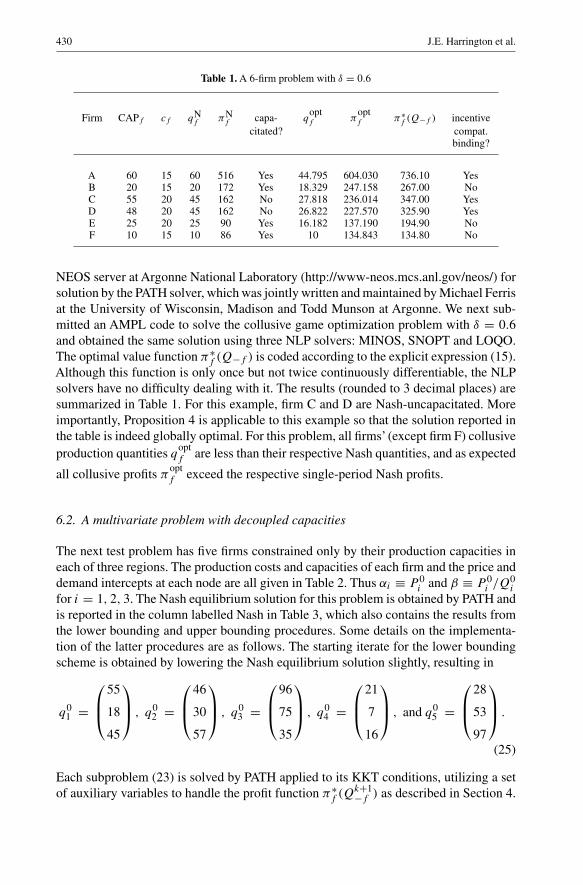
p(Q) ≡ 40− 0.08Q;the other data for the problem are summarized in Table 1. We wrote a simple AMPLprogram [8] to compute the Nash quantities qN

f for the firms and submitted it to the

430 J.E. Harrington et al.

Table 1. A 6-firm problem with δ = 0.6

Firm CAPf cf qNf πN

f capa- qoptf π

optf π∗f (Q−f ) incentive

citated? compat.binding?

A 60 15 60 516 Yes 44.795 604.030 736.10 YesB 20 15 20 172 Yes 18.329 247.158 267.00 NoC 55 20 45 162 No 27.818 236.014 347.00 YesD 48 20 45 162 No 26.822 227.570 325.90 YesE 25 20 25 90 Yes 16.182 137.190 194.90 NoF 10 15 10 86 Yes 10 134.843 134.80 No

NEOS server at Argonne National Laboratory (http://www-neos.mcs.anl.gov/neos/) forsolution by the PATH solver, which was jointly written and maintained by Michael Ferrisat the University of Wisconsin, Madison and Todd Munson at Argonne. We next sub-mitted an AMPL code to solve the collusive game optimization problem with δ = 0.6and obtained the same solution using three NLP solvers: MINOS, SNOPT and LOQO.The optimal value function π∗f (Q−f ) is coded according to the explicit expression (15).Although this function is only once but not twice continuously differentiable, the NLPsolvers have no difficulty dealing with it. The results (rounded to 3 decimal places) aresummarized in Table 1. For this example, firm C and D are Nash-uncapacitated. Moreimportantly, Proposition 4 is applicable to this example so that the solution reported inthe table is indeed globally optimal. For this problem, all firms’ (except firm F) collusiveproduction quantities qopt

f are less than their respective Nash quantities, and as expected

all collusive profits πoptf exceed the respective single-period Nash profits.

6.2. A multivariate problem with decoupled capacities

The next test problem has five firms constrained only by their production capacities ineach of three regions. The production costs and capacities of each firm and the price anddemand intercepts at each node are all given in Table 2. Thus αi ≡ P 0

i and β ≡ P 0i /Q

0i

for i = 1, 2, 3. The Nash equilibrium solution for this problem is obtained by PATH andis reported in the column labelled Nash in Table 3, which also contains the results fromthe lower bounding and upper bounding procedures. Some details on the implementa-tion of the latter procedures are as follows. The starting iterate for the lower boundingscheme is obtained by lowering the Nash equilibrium solution slightly, resulting in

q01 =

55

18

45

, q02 =

46

30

57

, q03 =

96

75

35

, q04 =

21

7

16

, and q05 =

28

53

97

.

(25)

Each subproblem (23) is solved by PATH applied to its KKT conditions, utilizing a setof auxiliary variables to handle the profit function π∗f (Q

k+1−f ) as described in Section 4.

Collusive game solutions via optimization 431

Table 2. Data for test problem 2

Node (Firm, node) cf i CAPf i P 0i Q0

i

1 40 5002 35 4003 32 640

(1,1) 15 300(1,2) 15 20(1,3) 15 50(2,1) 16 50(2,2) 16 400(2,3) 16 100(3,1) 12 200(3,2) 12 100(3,3) 12 40(4,1) 18 300(4,2) 18 20(4,3) 18 150(5,1) 14 30(5,2) 14 100(5,3) 14 400

The results in the lower-bound column in Table 3 are obtained after 28 iterations, withthe relative difference of the Nash bargaining objective at the last two iterations prior totermination being:

θ(qk+1)− θ(qk)θ(qk+1)

≈ 3.3582× 10−6.

Since the firms’ constraints are only regional production capacities, the optimal profitfunctions π∗f (Q−f ) can again be explicitly represented. However, since there are threeregions involved, each firm f has three decision variables qf i for i = 1, 2, 3; moreimportantly, the overall collusive game optimization problem (10) is not shown to be aconcave maximization problem. Nevertheless, most NLP solvers on NEOS were ableto solve the problem; in particular, SNOPT produces a solution that is very close to thatfrom the bounding procedures. The column labelled Upper Bound in Table 3 is obtainedfrom solving the penalized problem (18), modified in the following way. Using the vec-tor q0 in (25), we compute π∗f (q

0−f ) for all f ∈ F . We then fix all these optimal profits

and solve the resulting problem (18) by the NLP solver, SNOPT6.1, using ς = 1010,obtaining the solution presented in the upper-bound column in Table 3. While the sum of

the penalty terms after scaling the βi to be unity,∑

f∈F

(‖α −Q−f ‖2 − ξf

), is−0.09715

at termination, the computed solution in the modified upper bound problem neverthelesscoincides with that obtained from a direct solution of the problem (10) by an NLP solveron NEOS.

A major motivation in solving this test problem in different ways is to assess thequality of the solutions produced by the approaches. This assessment is useful becauseof the likely nonconvexity of the collusive optimization problem (10) being solved.With the three objective function values being very close to each other (cf. the last row

432 J.E. Harrington et al.

Table 3. Numerical results on test problem 2 with δ = 0.8

Variable Nash Lower Bound Upper Bound NLP

Generation q11 59 55.7603 55.7113 55.7113q12 20 11.6396 11.6915 11.6915q13 50 2.6264 2.6231 2.62312

total 129 70.0263 70.0259 70.0259

q21 46.5 50 50 50q22 30.2857 11.3264 11.2944 11.2944q23 57.5 0 0 0

total 134.2857 61.3263 61.2944 61.2944

q31 96.5 15.1505 15.1600 15.1600q32 76 100 100 100q33 40 40 40 40

total 212.5 155.1505 155.1600 155.1600

q41 21.5 29.3681 29.3557 29.3557q42 7.42875 0 0 0q43 17.5 0 0 0

total 46.42875 29.3681 29.3557 29.3557

q51 30 0 0 0q52 53.1429 0 0 0q53 97.5 138.9204 138.915 138.915

total 180.6429 138.9204 138.915 138.915

Profits firm 1 545.23 852.0030 852.0331 852.0331firm 2 418.5495 692.2188 692.1436 692.1436firm 3 1525.3798 1903.0242 1903.0818 1903.0818firm 4 57.1211 293.0262 293.0239 293.0239firm 5 894.0269 1239.5394 1239.5516 1239.5516

NBO θ(q) 0 2.584208E12 2.584210E12 2.584210E12

in Table 3), we are fairly confident that the obtained solution, which is not shown to beglobally optimal, is at least reasonable. This test also demonstrates the effectiveness ofthe two bounding procedures.

6.3. A multivariate problem with coupling capacities

Our third test problem involves the following coupling capacity constraint for each firm:

∑

i∈Nqf i ≤ CAPf . (26)

The data are the same as those in test problem 2; in addition, CAP1 = 200, CAP2 = 50,CAP3 = 200, CAP4 = 150, and CAP5 = 110. The starting iterate for the lower bound-ing scheme is obtained in the same way as before and is given as follows:

q01 =

67

51

80

, q02 =

24

12

12

, q03 =

67

51

80

, q04 =

35

22

30

, and q05 =

41

28

30

.

Collusive game solutions via optimization 433

In addition to the lower bounding procedure, we also ran the upper bounding procedurein the same way as in test problem 2. We have verified that the solution computed by thelatter procedure is feasible to (10); nevertheless, since the modified problem is not thetrue upper bound problem (18), we cannot conclude positively that the latter solution isglobally optimal to (10). See Table 4.

Finally, for comparison purposes, we use an NLP solver to directly solve an MPECformulation of the collusive game problem (10). Due to the aggregate capacities (26), theprofit function π∗f (Q−f ) no longer has an explicit representation. In order to deal withthis issue, we first observe that the problem (10) is equivalent to the following MPEC:

maximize∏

f∈F

(πf (q)− πN

f

)

subject to πf (q) ≥ ( 1− δ )[(q∗f )

T ( α − Diag(β) (Q−f + q∗f ) )− cTf q∗f]+ δ πN

f ,

0 ≤ 1T qf ≤ CAPf ,0 ≤ q∗f ⊥ Diag(β)Q−f + 2 Diag(β) q∗f − α + cf + γf ≥ 0,0 ≤ γf ⊥ CAPf − 1T q∗f ≥ 0.

Table 4. Numerical results on test problem 3 with δ = 0.8

Variable Nash solution Lower bound Upper Bound MPEC

Generation q11 67.2087 73.7309 73.7094 73.7100q12 51.9174 32.2374 32.2556 32.2537q13 80.8672 0 0 0

total 172.6016 105.9683 105.9650 105.9637

q21 24.5257 35.9905 35.9814 35.9731q22 12.8997 0 0 0q23 12.5745 0 0 0

total 50 35.9905 35.9814 35.9731

q31 67.2087 0 0 0q32 51.9241 0 0 0q33 80.8672 195.8417 195.8780 195.8765

total 200 195.7413 195.8780 195.8765

q41 37.2290 39.2440 39.2354 39.2392q42 24.5141 0 0 0q43 32.8999 0 0 0

total 94.6430 39.2440 39.2354 39.2392

q51 41.5989 0 0 0q52 28.5095 86.0862 86.0725 86.0721q53 39.8916 3.6629 3.6653 3.6665

total 110 89.7491 89.7378 89.7386

Profits firm 1 1044.5708 1275.5888 1275.7010 1275.7203firm 2 221.3998 434.8644 434.8677 434.7786firm 3 1644.5708 1963.2681 1963.2527 1963.2404firm 4 217.5821 395.6882 395.7245 395.7748firm 5 690.6684 945.9263 945.7592 945.7821

NBO θ(q) 0 7.1450994E11 7.145111E11 7.145107E11

434 J.E. Harrington et al.

In order to utilize an NLP solver, we rewrite the two complementarity constraints in theabove MPEC as follows:

( q∗f )T [ Diag(β)Q−f + 2 Diag(β) q∗f − α + cf + γf ] ≤ 0

( γf )T (CAPf − 1T q∗f ) ≤ 0.

The resulting nonlinear program remains nonconvex. Yet, SNOPT successfully termi-nated with a solution reported in the last column of Table 4. Notice that for this testproblem, the solutions produced by the lower and upper bounding scheme are very closeto that produced by SNOPT, thereby once again demonstrating the effectiveness of thebounding schemes. Note also the closeness of the NBO values produced by the twobounding schemes.

7. Conclusion

In this paper, we have introduced an optimization formulation for the collusive gameproblem and developed upper and lower bounding procedures for its global solution.We have also obtained numerical results that establish the effectiveness of the boundingprocedures in obtaining viable solutions, which are supported by publicly available NLPsolvers. As the collusive optimization problem is not shown to be convex in general, thebounding procedures, along with their theoretical properties established in Propositions 5and 8 and their ability to match the results from the NLP solvers, provide confidence onthe high fidelity of the numerical solutions obtained by all algorithms. The next step inour research should be application of the proposed model and algorithms to computationof equilibria for actual markets. This will be reported elsewhere.

Acknowledgements. This work is based on research partially supported by the National Science Foundationunder an EPNES grant ECS-0224817. The authors are very grateful to two referees who have made manyconstructive comments that have helped to improve the presentation and results of the paper.

References

1. Bernheim, B.D., Whinston, M.D.: Multimarket contact and collusive behavior. RAND J. Economics 21,1–26 (1990)

2. Bonnans, J.F., Shapiro, A.: Perturbation Analysis of Optimization Problems. Springer-Verlag, New York,2000

3. Bunn, D.W., Oliveira, F.S.: Evaluating individual market power in electricity markets via agent-basedsimulation. Ann. Oper. Res. 121, 57–77 (2003)

4. Danskin, J.M.: The theory of min-max with applications. SIAM J. Appl. Math. 14, 641–664 (1966)5. Dirkse, S.P., Ferris, M.C.: The PATH solver: A non-monotone stabilization scheme for mixed comple-

mentarity problems. Optimization Methods and Software 5, 123–156 (1995)6. Dubey, P.: Inefficiency of Nash equilibria. Math. Oper. Res. 11, 1–8 (1986)7. Facchinei, F., Pang, J.S.: Finite-Dimensional Variational Inequalities and Complementarity Problems.

Springer-Verlag, New York, 20038. Fourer, R., Gay, D.M., Kernighan, B.W.: AMPL: A Modeling Language for Mathematical Programming.

Duxbury Press, Brooks/Cole Publishing Company, 20029. Friedman, J.W.: Oligopoly and the Theory of Games. North-Holland, Amsterdam, 1977

10. Fudenberg, D., Tirole, J.: Game Theory. MIT Press, Cambridge, 1991

Collusive game solutions via optimization 435

11. Harrington, J.E., Jr.: Collusion in multiproduct oligopoly games under a finite horizon. InternationalEconomic Review 28, 1–14 (1987)

12. Harrington, J.E., Jr.: The determination of price and output quotas in a heterogeneous cartel. InternationalEconomic Review 32, 767–792 (1991)

13. Herrero, M.J.: The Nash program: non-convex bargaining problems. J. Economic Theory 49, 266–277(1989)

14. Horst, R., Thoai, N.V.: DC programming: Overview. J. Optimization Theory and Applications 103, 1–43(1999)

15. Kaneko, M.: An extension of the Nash bargaining problem and the Nash social welfare function. Theoryand Decision 12, 135–148 (1980)

16. Luo, Z.Q., Pang, J.S., Ralph, D.: Mathematical Programs With Equilibrium Constraints. Cambridge Uni-versity Press, Cambridge, England, 1996

17. Nash, J.F.: The bargaining problem. Econometrica 28, 155–162 (1950)18. Osborne, M.J., Rubinstein, A.: Bargaining and Markets. Academic Press, San Diego, 199019. Puller, S.L.: Pricing and firm conduct in California’s deregulated electricity market. PWP-080, Power

Program, University of California Energy Institute, Berkeley, 200120. Rockafellar, R.T., Wets, R.J.-B.: Variational Analysis. Springer-Verlag, Berlin, 199821. Rothkopf, M.H.: Daily repetition: A neglected factor in the analysis of electricity auctions. The Electricity

J. 12, 61–70 (1999)22. Schmalensee, R.: Competitive advantage and collusive optima. International J. Industrial Organization 5,

351–367 (1987)23. Sweeting, A.: Market outcomes and generator behaviour in the England and Wales wholesale electricity

market, 1995-2000. Department of Economics, Massachusetts Insitute of Technology, presented at the7th Annual POWER Research Conference on Electricity Industry Restructuring, University of CaliforniaEnergy Institute, Berkeley, March 22, 2002

24. Tao, P.D., An, L.T.H.: A d.c. optimization algorithm for solving the trust-region subproblem. SIAMJournal on Optimization 8, 476–505 (1998)

25. Tawarmalani, M., Sahinidis, N.V.: Convex extensions and envelopes of lower semi-continuous functions.Mathematical Programming, Series A 93, 247–263 (2002)

26. Tawarmalani, M., Sahinidis, N.V.: Convexification and Global Optimization in Continuous and Mixed-Integer Nonlinear Programming: Theory, Algorithms, Software, and Applications. (Kluwer AcademicPublishers, Dordrecht, 2002). [Volume 65 in “Nonconvex Optimization And Its Applications” series.]