Prepared for submission to JHEP UUITP-52/19, LCTP-19-35

On Positive Geometry and Scattering Forms for

Matter Particles

Aidan Herderschee,a Song He,b,c Fei Tengd and Yong Zhangb,e,c

aLeinweber Center for Theoretical Physics,

Randall Laboratory of Physics, Department of Physics,

University of Michigan, Ann Arbor, MI 48109, USAbCAS Key Laboratory of Theoretical Physics, Institute of Theoretical Physics, Chinese Academy

of Sciences, Beijing 100190, ChinacSchool of Physical Sciences, University of Chinese Academy of Sciences, No.19A Yuquan Road,

Beijing 100049, ChinadDepartment of Physics and Astronomy, Uppsala University, 75108 Uppsala, SwedenePerimeter Institute for Theoretical Physics, Waterloo, ON N2L 2Y5, Canada

E-mail: aidanh@umich.edu, songhe@itp.ac.cn, fei.teng@physics.uu.se,

yongzhang@itp.ac.cn

Abstract: We initiate the study of positive geometry and scattering forms for tree-

level amplitudes with matter particles in the (anti-)fundamental representation of the

color/flavor group. As a toy example, we study the bi-color scalar theory, which sup-

plements the bi-adjoint theory with scalars in the (anti-)fundamental representations of

both groups. Using a recursive construction we obtain a class of unbounded polytopes

called open associahedra (or associahedra with certain facets at infinity) whose canonical

form computes amplitudes in bi-color theory, for arbitrary number of legs and flavor as-

signments. In addition, we discuss the duality between color factors and wedge products,

or “color is kinematics”, for amplitudes with matter particles as well.

arX

iv:1

912.

0830

7v2

[he

p-th

] 1

Feb

202

0

Contents

1 Invitation: bi-color scalars and open associahedra 1

2 Review 6

2.1 Kinematic Associahedron 6

2.2 Scattering Forms and “Color is Kinematics” 8

2.3 Color Ordered Amplitudes with both Adjoint and Fundamental Particles 10

2.4 Bi-color φ3 Amplitudes 11

3 Open Associahedra in Kinematic Space 12

3.1 Special Color Orderings 14

3.2 Generic Recursive Construction 19

3.3 Remarks 25

4 “Color is Kinematics” for (Anti-)Fundamental States 26

4.1 (Anti-)Fundamental Small Kinematic Space 26

4.2 Duality between Differential Forms and Color Factors 29

4.3 (Non-)Projectivity of the Scattering Form 31

4.4 Melia Decomposition Dual to Pullback 32

5 Conclusion 34

A Possible Deformations on Constraints 36

B Explicit Factorization Examples 38

C Derivation of dim(Kkn) 39

D Explicit Form of HAn [α] 40

1 Invitation: bi-color scalars and open associahedra

In [1], a novel geometric understanding, which resembles the amplituhedron for the planar

N = 4 SYM [2, 3], has been proposed for scattering amplitudes in various massless theories

in general spacetime dimension. The key idea is, instead of considering amplitudes as

functions, they are most naturally thought of as differential forms on the kinematic space

spanned by Mandelstam variables. In particular, tree-level amplitudes of bi-adjoint φ3

theory are given by the canonical form [4] of a classic polytope – the associahedron, living

naturally in a subspace of the kinematic space. In this so-called ABHY (Arkani-Hamed,

Bai, He, Yan) realization of the kinematic associahedron, the usual Feynman-diagram

– 1 –

expansion in terms of planar cubic tree graphs corresponds to a particular triangulation,

and the geometric picture allows us to see hidden symmetry and obtain new formula, even

for planar φ3 amplitudes [5].

More generally, for tree amplitudes in any massless theories with adjoint particles,

such as Yang-Mills theory (YM) or U(N) non-linear sigma models (NLSM), the scattering

forms on kinematic space are dual to the fully color-dressed amplitudes despite having no

explicit color factors. This is due to the fact that wedge products of Mandelstam variables

in the scattering forms satisfy the same Jacobi relations as color factors, a statement

dubbed “Color is Kinematics”; relatedly, the usual trace decomposition was shown to be

equivalent to pullback of scattering forms to subspace for the associahedron of a planar

ordering. All these scattering forms are d log forms for φ3 diagrams dressed with kinematic

numerators, and requiring them to be well-defined on the projectivized kinematic space

leads to a geometric origin for color-kinematics duality.

A natural question is how general is this geometric picture for scattering amplitudes.

For example, can it be extended to more general theories, such as QCD, which have particles

in the (anti-)fundamental representations? Since we work in general dimensions where

mass can be obtained via dimensional reduction, it is convenient to restrict to the massless

case.1 Recently there has been progress in the study of QCD amplitudes in the context

of color-kinematics duality and double copy of Bern-Carrasco-Johansson (BCJ) [6]. In

particular, a generalization of bi-adjoint φ3 theory has been proposed, which includes

scalars in the (anti-)fundamental representations of both groups, e.g., U(N) × U(N ′) [7].

We use [T a, T b] = fabcT c and tr(T aT b) = δab as the normalization of Lie algebra generators

and structure constants. The Lagrangian reads:

Lφ3 =1

2∂µφ

aA∂µφaA +λ

6fabcfABCφaAφbBφcC

+

nf∑r=1

[∂µ(ϕr)iI∂

µ(ϕ∗r)iI + λφaA(ϕ∗r)

iI(T a)ji (TA)JI (ϕr)jJ

], (1.1)

where λ is an arbitrary coupling constant, r is the flavor index of the complex scalar ϕ,

and nf is the total number of flavors. The real scalar φ carries adjoint representation

indices (a,A) of the symmetry group U(N) × U(N ′), while ϕ and ϕ∗ carry fundamental

representation indices (i, I) and anti-fundamental ones (i, I) respectively. More details will

be given in section 2.4. Among other things, amplitudes of such bi-color scalars play an

important role for KLT-type double copy relations for QCD amplitudes [8, 9], just as the

original KLT relations have the bi-adjoint φ3 amplitudes as the central object [10, 11].

In this paper, we initiate systematic studies of a geometric picture for amplitudes with

(anti-)fundamental particles by considering tree amplitudes of the bi-color scalar theory.

There is a direct generalization of the kinematic associahedron, which computes bi-color

scalar amplitudes, and the statement “color is kinematics” also extends to these cases.

Recall that for any assignment of adjoint and (anti-)fundamental particles, flavor de-

1More precisely, the results in this paper will not change if fundamental representation particles acquiremass from a dimensional reduction.

– 2 –

composition of the amplitude for both U(N) and U(N ′) lead to a matrix of bi-color scalar

(double-partial) amplitudes m[α|β], where α and β denote the orderings; m[α|β] is given

by a sum of trivalent tree graphs, which are determined by the collection of all poles com-

patible with both orderings and the flavor structure for particles in the (anti-)fundamental.

For simplicity, we restrict ourselves to the diagonal case with α = β = (12 · · ·n), An :=

m[12 · · ·n | 12 · · ·n], since more general cases can be viewed as the intersection of diagonal

cases [8, 11–13]. In the special case with only bi-adjoint particles, the amplitude is given by

the sum of all (Catalan number of) planar cubic tree graphs, which contain all n(n−3)/2

planar variables since there is no restriction from flavor structures. As we will review

shortly, the bi-adjoint φ3 amplitude is given by the canonical form of a (n−3)-dim associa-

hedron in kinematic space; the latter is the intersection of (1) the top-dimensional cone with

all planar variables being positive, and (2) an (n−3)-dim subspace given by all non-adjacent

si,j with 1 6 i < j < n being negative constants (n(n−3)/2− (n−3) = (n−2)(n−3)/2 con-

straints in total) [1].

As a main result of this paper, which will be presented in section 3, we obtain any

general bi-color amplitude An as the canonical form of an open associahedron, i.e. an

associahedron with faces sent to infinity. In fact, such open associahedra already appear

for off-diagonal m[α|β] for bi-adjoint cases [1], and our results are a generalization in the

presence of k pairs of (anti-)fundamental particles with distinct flavors. Out of all the

n(n−3)/2 planar poles, only N of them are allowed by the flavor structure and color

ordering while the remaining ones are set to positive constants. Almost identical to the

bi-adjoint case, we can construct any open associahedron as the intersection of an N-

dim positive cone with N 6 n(n−3)/2 and a (n−3)-dim subspace given by N − (n−3)

constraints that are still in the form of setting certain Mandelstam variables to negative

constants. Very interestingly, these constraints can be given by a recursive procedure that

generalizes the “inverse soft construction” of the bi-adjoint associahedra. We can fix the

entire open associahedra through the analysis of two factorization channels (facets) at each

step. The basic observation we have is that the pullback of planar scattering form to

the subspace gives the canonical form of open associahedron, which consists of only those

Feynman diagrams allowed by the flavor structure.

Let’s present a few explicit examples to illustrate the simplicity of our construction,

and the detailed discussion will be given in section 3.2. We put labels 1, 2, . . . , n on the

boundary of a disk, and represent the flavor structure by connecting each pair of particles in

the (anti-)fundamental by a directed line. For example, for n = 4 we have three possibilities

with k = 0, 1, 2. Note that k = 1 case is identical to the bi-adjoint (k = 0) case, and both

consist of two Feynman diagrams with s = s1,2, t = s2,3 channels,

A4

1

2 3

4

=1

s+

1

t, A4

1

2 3

4

=1

s+

1

t. (1.2)

The disk graphs stand for the sum of all Feynman diagrams with cyclically ordered fun-

– 3 –

damental, anti-fundamental, and adjoint states. The corresponding associahedron is an

interval given by:

AAA4

1

2 3

4

=AAA4

1

2 3

4

= s > 0, t > 0, u = −s− t = −c , (1.3)

where c is a positive constant. The pullback of the planar form d log st |s+t=c = ds(1

s + 1t ) is

the canonical form of the interval, which gives the amplitude. However, for the k = 2 case

with e.g. 1,2 and 3,4 as two pairs of bi-fundamental scalars, the t-pole is forbidden by

conservation of flavors and there is only one Feynman diagram left,

A4

1

2 3

4

=1

s, AAA4

1

2 3

4

= s > 0, t = b > 0 . (1.4)

Here we see the simplest example of open associahedron, a half line from s = 0 to infinity,

which corresponds to setting the other boundary t = 0 to infinity. The pullback of d log s/t

to the space gives the canonical form d log s = ds/s (and the correct amplitude). In this

case, the forbidden pole t is set to a positive constant b, and we have only N = 1 pole s so

there is no need to further specify a subspace. This amplitude and open associahedron are

identical to those for the bi-adjoint off-diagonal case m[1234|1243] [1].

To give further examples of our results, we need to introduce some notations. Through-

out the paper, we use the following definition of Mandelstam variables:

si,j,k,l,... := (pi + pj + pk + pl + . . .)2 . (1.5)

The subscript can also be sets:

sA,B,C,D,... :=( ∑i∈A∪B∪C∪D∪...

pi

)2. (1.6)

The planar Mandelstam variable Xi,j is defined as

Xi,j := si,i+1,...,j−1 = (pi + pi+1 + . . .+ pj−1)2 , (1.7)

such that on the support of momentum conservation Xi,j = Xj,i.

As we will see shortly, it is convenient to first consider amplitudes with only bi-

fundamental scalars, i.e., the case with n = 2k. These represent the most non-trivial

part of our construction, with adding bi-adjoint scalars relatively easier. Among such pure

bi-fundamental scalar amplitudes, the simplest one correspond to the case where the k

pairs of particles form parallel lines. As shown in eq. (1.8), they correspond to two pairs

at two ends, (1, 2), (k+1, k+2), and k−2 pairs in between, (i, n+3−i) for i = 3, · · · , k. It

– 4 –

is straightforward to see that the flavor structure allows k−1 propagators of the bi-adjoint

type and 2(k − 2) ones of the bi-fundamental type (N = 3k−5 poles in total); there are

2k−2 Feynman diagrams as follows:

An

n−1

n

1

2

3 4kk+1

k+2k+3

· · ·

=

1

X1,3

k∏i=3

(1

Xi,n+3−i+

1

Xi+1,n+4−i

)1

Xi+1,n+3−i. (1.8)

In other words, the amplitude factorizes as the product of k−1 factors of 1s and k−2 factors

of 1s + 1

s . The corresponding open associahedron must be the direct product of k−1 half-

lines and k−2 intervals. It is nice that the subspace is given by setting the k−2 = N−(n−3)

Mandelstam variables for the non-adjacent pairs, i.e. si,n+3−i, to negative constants:

HHHn

n−1

n

1

2

3 4kk+1

k+2k+3

· · ·

=

k⋃i=3

−si,n+3−i = ci,n+3−i > 0 . (1.9)

Requiring the N allowed poles to be positive, together with these subspace constraints,

gives the open associahedron whose canonical form is the correct amplitude.

For n = 2k, the situation gets more interesting when we go beyond the parallel case,

and the first such example is with three adjacent bi-fundamental pairs for n = 6, where we

have N = 6 allowed poles and four Feynman diagrams

A6

1

2

3 4

5

6

=1

X1,3X3,5X1,5+

1

X1,3X3,5X3,6+

1

X1,3X1,4X1,5+

1

X3,5X2,5X1,5.

(1.10)

Remarkably, the open associahedron is given by the subspace with N − 3 = 3 constraints,

which set three-particle Mandelstam variables to negative constants:

HHH6

1

2

3 4

5

6

= s2,5,6, s3,5,6, s3,4,6 set to negative constants . (1.11)

The construction for open associahedron becomes more complicated as k and n increase.

However, there exists a nice recursive procedure that allows us to insert a bi-adjoint scalar

– 5 –

or an adjacent pair of bi-fundamental scalars. For example, for the following configura-

tions with n = 7 and n = 8, we have N = 11 and N = 14 allowed poles respectively,

X1,3, X1,4, X1,5, X1,6, X2,5, X2,7, X3,5, X3,6, X3,7, X4,7, X5,7, X1,3, X1,4, X1,5, X1,6, X1,7,

X2,5, X2,7, X3,5, X3,6, X3,7, X3,8, X4,7, X5,7, X5,8; here we present their subspaces with 7

and 9 constraints respectively:

HHH7

1

2

3

4 5

6

7

=

s2,5,6, s3,5,6, s3,4,6, s2,7, s3,7, s4,7, s5,7

set to negative constants

, (1.12)

HHH8

1

2

3

4 5

6

7

8

=

s2,5,6, s3,5,6, s3,4,6, s2,7,8, s3,7,8, s4,7,8, s5,7,8, s3,4,8, s5,6,8

set to negative constants

. (1.13)

We will show in section 3 how to derive these constraints from the recursive procedure.

As our last example in the introduction, here we present a more involved case for n =

11, k = 4, which has N = 22 allowed poles, X1,3, X1,4, X1,6, X1,7, X1,8, X1,9, X1,10, X2,8, X3,6,

X3,7, X3,8, X3,9, X3,10, X3,11, X4,6, X4,7, X4,8, X5,7, X6,8, X8,10, X8,11, X9,11, and the subspace

is given by 14 constraints

HHH11

1

2

3

45 6 7

8

9

1011

=

s3,6, s4,6, s3,7, s4,5,7, s8,10, s2,8,9,10,11, s3,8,9,10,11,

s4,5,8,9,10,11, s6,8,9,10,11, s3,4,5,6,7,11, s8,11, s9,11,

s3,4,5,6,7,9, s3,4,5,6,7,10

set to negative constants

. (1.14)

The outline of this paper is as follows. We first review kinematic associahedron and bi-

color theory in section 2. Then we derive the subspace for above examples, ending up with

the constructions of subspace for most general cases of bi-color theory in section 3. Some

deformed versions of subspace and explicit factorization examples are put in appendix A

and B. In section 4, we show how “color is kinematic” for the color-dressed amplitudes of

bi-color theory, with some details put in appendix C and D.

2 Review

2.1 Kinematic Associahedron

A prime example of an amplitude that is the canonical form of a polytope is the case of the

associahedron for bi-adjoint scalar theory, as discovered in [1]. Here we give a brief review

of it. In large enough spacetime dimensions, the kinematic space of n massless particles,

Kn, can be spanned by all independent si,j ’s, thus it has dimension d = n(n−3)/2. Since

there are n(n− 3)/2 planar poles Xi,j with i+ 1 < j in a cyclic ordering in the bi-adjoint

scalar amplitude m[12 · · ·n | 12 · · ·n], we can start with the top cone where all planar poles

– 6 –

are positive. The remaining objective is to find a (n − 3)-dimension hyperplane whose

intersection with the cone gives the associahedron.

The hyperplane can be expressed by d − (n − 3) = (n − 2)(n − 3)/2 constraints. As

described in [1], one way to construct the hyperplane is to set all −si,j = Xi,j +Xi+1,j+1−Xi,j+1 − Xi+1,j with 1 6 i < i + 1 < j 6 n − 1 to positive constants. For example,

for the four-point case (1.2), the 2-dim cone is s > 0, t > 0 and the 1-dim subspace is

u = −s− t = −c. Their intersection is an interval, which is a 1-dim associahedron.

In the following paper, we will often see the intersection of a subspace and a cone or

another subspace,

P = Q ∩R , (2.1)

where P,Q,R can be described by sets of constraints. In geometry, polytope P is indeed

an intersection of two others. However, algebraically, we can say the set of constraints PPP

for the polytope P is the union of those of Q and R,

PPP = QQQ ∪RRR . (2.2)

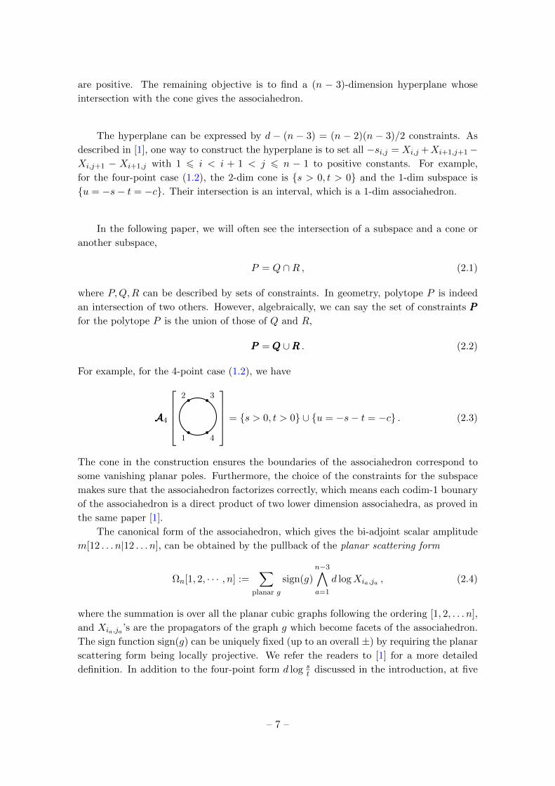
For example, for the 4-point case (1.2), we have

AAA4

1

2 3

4

= s > 0, t > 0 ∪ u = −s− t = −c . (2.3)

The cone in the construction ensures the boundaries of the associahedron correspond to

some vanishing planar poles. Furthermore, the choice of the constraints for the subspace

makes sure that the associahedron factorizes correctly, which means each codim-1 bounary

of the associahedron is a direct product of two lower dimension associahedra, as proved in

the same paper [1].

The canonical form of the associahedron, which gives the bi-adjoint scalar amplitude

m[12 . . . n|12 . . . n], can be obtained by the pullback of the planar scattering form

Ωn[1, 2, · · · , n] :=∑

planar g

sign(g)

n−3∧a=1

d logXia,ja , (2.4)

where the summation is over all the planar cubic graphs following the ordering [1, 2, . . . n],

and Xia,ja ’s are the propagators of the graph g which become facets of the associahedron.

The sign function sign(g) can be uniquely fixed (up to an overall ±) by requiring the planar

scattering form being locally projective. We refer the readers to [1] for a more detailed

definition. In addition to the four-point form d log st discussed in the introduction, at five

– 7 –

points we have

Ω5[1, 2, 3, 4, 5] = d logX1,4 ∧ d logX1,3 + d logX1,3 ∧ d logX3,5 + d logX3,5 ∧ d logX2,5

+ d logX2,5 ∧ d logX2,4 + d logX2,4 ∧ d logX1,4 . (2.5)

Similarly, we can define the α-planar scattering form as

Ωn[α] :=∑

α-planar g

sign(g|α)n−3∧a=1

d logXα(ia),α(ja) (2.6)

which can be obtained from eq. (2.4) by a permutation α. Locality and unitarity is manifest

in the associahedron. In addition, “color is kinematics” in this representation, as we will

review next.

2.2 Scattering Forms and “Color is Kinematics”

Now we review the definition of the full scattering form, which is the natural generaliza-

tion of eq. (2.6). The full scattering form encodes nontrivial kinematic numerators and all

the color orderings. For convenience, we denote the collection of all cubic tree Feynman

diagrams with n external legs as Γn. Each g ∈ Γn is specified by n−3 mutually compat-

ible propagators. We denote them as sI , where I ∈ g are associated with the internal

propagators. We define their wedge product as:

W (g|αg) := sign(g|αg)∧I∈g

dsI (2.7)

where αg is a color ordering compatible with g. The overall sign depends on ordering of

the ds’s. Both W (g|αg) and sign(g|αg) satisfy the mutation and vertex flip rule [1].

The full scattering form is defined as an (n−3)-form in Kn: a linear combination of

d log’s of propagators for each diagram,

Ωn[N ] :=∑g∈Γn

N(g|αg)W (g|αg)∏I∈g

1

sI, (2.8)

where for any three graphs as in figure 1, we require their numerators satisfy

N(gS |I1I2I3I4) +N(gT |I1I4I2I3) +N(gU |I1I3I4I2) = 0 . (2.9)

This requirement guarantees that the scattering form is projective [1], i.e. it is invariant

under a GL(1) transformation sI → Λ(s)sI for all subsets I (with Λ(s) depending on s).2

An explicit example of the scattering form (2.8) is given by eq. (2.6) where the numera-

tors are simply sign(g|α) if the diagram is compatible with α and 0 otherwise. Its pullback

to a subspace is the canonical form of an associahedron. More examples of differential

forms whose pullback are the canonical form of polytopes are given in [1, 14, 15]. Note

2Here the GL(1) transformation will not be applied to the numerators N(g|αg). A restrict descriptionis to use another kind of variables in the so-called big kinematic space [1]. We postpone it to section 4.1

– 8 –

I1 I2

I3I4

I1 I4

I2I3

I1 I3

I4I2

S = sI1,I2 T = sI2,I3 U = sI1,I3

gS gT gU

Figure 1. A triplet of three cubic tree graphs that differ by one propagator.

that a linear combination of scattering forms is still a scattering form. For example, one

can construct the scattering forms for YM and NLSM this way [1].

For any triplet gS , gT , gU of graphs that differ only by one propagator, as shown in

figure 1, there is a so-called seven-term identity implied by momentum conservation,

sI1,I2 + sI2,I3 + sI1,I3 = sI1 + sI2 + sI3 + sI4 , (2.10)

where the four propagators connecting to the four subgraphs are denoted as sI1 , . . . , sI4 .

This leads to an identity that their wedge products satisfy the Jacobi identity that is

equivalent to those of color factors,

W (gS |I1I2I3I4)+W (gT |I1I4I2I3)+W (gU |I1I3I4I2) = · · ·∧(dS+dT+dU)∧· · · = 0 , (2.11)

where the distinct Mandelstam variables are S, T, U , respectively, and “· · · ” denotes the

wedge products of the remaining n−4 propagators shared by the three graphs. Eq. (2.11)

implies a duality between color factors and differential forms on kinematic space Kn:

C(g|αg) ↔ W (g|αg) . (2.12)

Hence “color is kinematics”. Considering a color-dressed amplitude Mn,

Mn[N ] =∑g∈Γn

N(g|αg)C(g|αg)∏I∈g

1

sI, (2.13)

the duality (2.12) leads naturally to a duality between color-dressed amplitudes and scat-

tering forms,

Mn[N ] ↔ Ωn[N ] . (2.14)

In addition, a color-ordered amplitude can be obtained by pulling back the scattering form

Ωn onto an appropriate subspace [1].

– 9 –

2.3 Color Ordered Amplitudes with both Adjoint and Fundamental Particles

A color ordered amplitude An[α] only receives contributions from the Feynman diagrams

that contain no crossing edges when the external particles are put on a circle according to

the ordering α. In particular, each particle in fundamental (f) representation is connected

to its anti-fundamental (af) partner by a directed line representing the color flow. For

example, we have

A6[1, 2, 3, 4, 5, 6] = A6

1

2

3 4

5

6

, A8[1, 2, 3, 4, 5, 6, 7, 8] = A8

1

2

34

5

6

78

,

(2.15)

where we use underscores (bars) to denote f (af) particles.3 We further require that the

f particles always come before their af partners in α. This is because we can always use

these color ordered amplitudes to linearly expand those with flipped pairs [16]. For most

parts of this paper, we assume each f-af pair carries a distinct flavor. The single flavor

case can be recovered by averaging over different flavor assignments.

By associating each f particle with an open parenthesis and each af one with a closed

parenthesis, we can convert an ordering α into a Dyck word with adjoint-representation

(adj) particle insertions, the whole set of which is denoted as Dyckn,k for n external particles

and k f-af pairs. We call an f-af pair (l, r) adjacent in α if there exists an i that α(i) = l

and α(i+1) = r. The orderings given in eq. (2.15) can thus be written as [(1, 2, 3), (4, 5, 6)]

and [(1, (2, 3), 4, 5), (6, 7, 8)]. In the second ordering, the f-af pair (2, 3) is adjacent. In this

work, we study the color orderings that are given by Dyckn,k modulo cyclicity:

MMMn,k = Dyckn,k/cyclic permutations, (2.16)

namely, two color orderings are considered the same if they differ by a cyclic permutation

that respects the parenthesis structure. For example, both orderings in eq. (2.15) have two

equivalent representations:

[(1, 2, 3), (4, 5, 6)] ∼ [(4, 5, 6), (1, 2, 3)] ,

[(1, (2, 3), 4, 5), (6, 7, 8)] ∼ [(6, 7, 8), (1, (2, 3), 4, 5)] . (2.17)

At k = 0, MMMn,k returns to the usual trace basis for adj particles. The size of MMMn,k is

(n− 1)!/k! [17].

As a basis, MMMn,k is redundant since there exist linear relations between color ordered

amplitudes. If there are no f-af pairs, the minimal basis under the color Lie algebra is the

Del Duca-Dixon-Maltoni (DDM) basis [18], given by An[1, 2, σ] with σ a permutation of

3When the ordering of states is arbitrary, we will denote flavor pairs using capital letters, like A and A.

– 10 –

the rest n−2 particles. For k > 1, we can by convention label one f-af pair as (1, 2). The

minimal basis under the color Lie algebra is the Melia basis, in which the pair (1, 2) always

comes first [16, 19, 20]: α = [(1, 2), σ]

∣∣σ ∈ Dyckn−2,k−1

. (2.18)

The size of Melia basis is (n− 2)!/k!. We can write an ordering α in the Melia basis as

α = [(1, 2),B2,B3, . . . ,Bm] = [B1,B2,B3, . . . ,Bm] , (2.19)

where each Bi is a block, and we always fix B1 = (1, 2) in the Melia basis. The block Bican either be an adj block, which contains a single adj particle gi: Bi = gi, or an f-af block,

which is defined as a Dyck word (with adj particle insertions) that is enclosed by an overall

parenthesis. The simplest f-af block contains just an adjacent f-af pair Bi = (li, ri). In

general, it has substructures:

Bi = (li,Bi1 ,Bi2 , . . . ,Bis , ri) , li ∈ f and ri ∈ af , (2.20)

where each Bi` is again a block, but for future convenience we call it a sub-block of Bi.

The definition of a block is thus recursive and it terminates when we reach an adj block or

an adjacent f-af pair. We define sub[Bi] as the collection of all the sub-blocks of Bi. For

example, if Bi is given by eq. (2.20), we have

sub[Bi] = Bi1 ,Bi2 , . . . ,Bis . (2.21)

It is also convenient to view an adj block Bi = gi as a degenerate limit of an f-af block,

in which li = ri = gi and sub[Bi] = ∅. Pictorially, a block Bi is represented by all the

structures bounded by the line (li, ri).

2.4 Bi-color φ3 Amplitudes

The above discussion applies to generic color ordered amplitudes, for example, QCD. Now

we move on to some features peculiar to the amplitudes of the bi-color scalar theory whose

Lagrangian are given by eq. (1.1). We introduce a flavor function that returns the abstract

flavor symbol of the fields:

f(ϕr) = fr , f(ϕ∗r) = −fr , f(φ) = 0 , (2.22)

where each fr is non-numeric and distinct in the sense that fa ± fb with a 6= b is kept

unevaluated. With the help of this flavor function, we can define

ϑI =

1

∑s∈I f(s) = 0 or a single term ± fr

0 otherwise, (2.23)

such that a propagator 1/sI is allowed by flavor conservation if and only if ϑI = 1.

– 11 –

We can expand the full color-dressed amplitude of the theory (1.1) by doubly color-

ordered amplitudes m[α|β]. In this paper, we will mainly study the diagonal component

An[α] := m[α|α]. The major simplification in this scalar theory is that the kinematic

numerator is trivial. As a result, color ordered amplitudes do not distinguish particles and

anti-particles, for example, A6[1, 2, 3, 4, 5, 6] = A6[1, 2, 3, 4, 5, 6], although the color factors

of these two cases are different. While this feature does not change the size of MMMn,k, and

the minimal Melia basis is still the same, each ordering in MMMn,k potentially gets more

equivalent representations. This is because we can flip the parentheses if necessary. For

example, we now have

[(1, 2, 3), (4, 5, 6)] ∼ [2, (3, (4, 5, 6), 1)] , etc,

[(1, (2, 3), 4, 5), (6, 7, 8)] ∼ [(2, 3), 4, (5, (6, 7, 8), 1)] , etc, (2.24)

both of which are not valid for generic color ordered amplitudes like QCD. Nevertheless,

for the bi-color scalar theory (1.1), We can use this enlarged cyclic freedom to represent

any α ∈MMMn,k as

α = [B1,B2,B3, . . . ,Bm] , where either B1 = (l1, r1) or B1 = g1 . (2.25)

The B1 = g1 case is always possible if adj particles are present. Otherwise, there must

exist at least one adjacent f-af pair, which we can identify as B1 = (l1, r1). If all f-af pairs

are adjacent in α, then for each block Bi in α we either have Bi = (li, ri) or Bi = gi.

For generic configurations, the representation is usually not unique, but any one of the

equivalence class will work for our purpose.

3 Open Associahedra in Kinematic Space

We now construct the kinematic polytope associated to the tree-level φ3 amplitudes of the

bi-color theory (1.1). The discussion here applies to amplitudes with a pair of the same

ordering α ∈MMMn,k.

To start with, we define ∆n[α] as a positive region in kinematic space where all the

α-planar variables forbidden by the flavor assignment are set to positive constants. It can

be written as ∆n[α] = Pn[α] ∩ Fn[α], where the subspace Pn and Fn are given by the

constraints

(positivity constraints) PPPn[α] =Xα(i),α(j) > 0 for all 1 6 i < j 6 n

, (3.1)

(flavor constraints) FFFn[α] =Xα(i),α(j) = bα(i),α(j) > 0 if ϑα(i),...,α(j−1) = 0

,

and ϑ is given in eq. (2.23). The constraints that carve out the region ∆n[α] are given by

∆∆∆n[α] = PPPn[α] ∪FFFn[α]. The flavor constraints, present when there are more than two f-af

pairs, remove all the Feynman diagrams that violate the flavor conservation from the α-

planar scattering form (2.6). These forbidden poles can easily be visualized in the polygon

dual to Feynman diagrams. For each f-af pair(α(i), α(j)

), we draw a line connecting the

– 12 –

edge Eα(i),α(i+1) and Eα(j),α(j+1), called a flavor line. Then a pole Xa,b is forbidden by

flavor conservation if the diagonal (a, b) crosses two or more flavor lines. Two examples are

given in figure 2. The dimension of ∆n[α] is

n− 3 6 dim∆n[α] 6n(n− 3)

2− k(k − 1)

2, (3.2)

where k is the number of f-af pairs. The first equality only holds when n=4 and k=2. The

maximal dimension of ∆n[α] is reached

if all the f-af pairs are adjacent in α: dim∆n[α] =n(n− 3)

2− k(k − 1)

2. (3.3)

To obtain the (n−3)-dimensional kinematic polytope An[α], we need to further restrict

∆n[α] to a subspace Hn[α]:

(subspace) An[α] = Hn[α] ∩∆n[α] ,

(set of constraints) AAAn[α] = HHHn[α] ∪∆∆∆n[α] . (3.4)

For k = 1, since the amplitude is the same as the pure bi-adjoint one, the subspace Hn[α]

is also the same, given by the constraints:

HHHn[(1, 2), 3, . . . , n] = −si,j = ci,j > 0 for non-adjacent pairs in 2 6 i < j 6 n . (3.5)

The resultant kinematic polytope An[α] is just the associahedron [1]. The restriction

equations for the original ABHY associahedra can be derived in a number of ways, each

with their own generalizations [1, 21, 22]. We will focus on the inverse soft construction of

associahedra [14], as this construction has a natural generalization for open associahedra.

Although it was originally derived by considering how CHY integrands behave under soft

limits, the inverse-soft construction is still applicable to bi-color amplitudes with both

adjoint and (anti-)fundamental states, which currently lack a clear CHY picture, due to

its geometric interpretation. Starting from HHHn−1, the original inverse-soft construction for

closed associahedra fixes HHHn by imposing

• The facet of the X1,n−1 = sn−1,n → 0 factorization channel of An must be An−1.

This can be done by inheriting all the constraints in HHHn−1.

• Additional constraints inHHHn must ensure that the facet X1,n−1 does not intersect the

facets of the channels incompatible to it. This can be done by setting the non-planar

Mandelstam variables in certain seven-term identities to a negative constant.

In the case of closed associahedra, the inverse soft construction yields [14]

HHHn := HHHn−1 ∪ −si,n = ci,n > 0 | 2 6 i 6 n− 2 . (3.6)

Together with HHH3 = ∅ it is enough to fix the restriction equations of An. Using the explicit

forms of the restriction equations, one can directly prove that An has the correct structure.

– 13 –

1

2

3

4

5

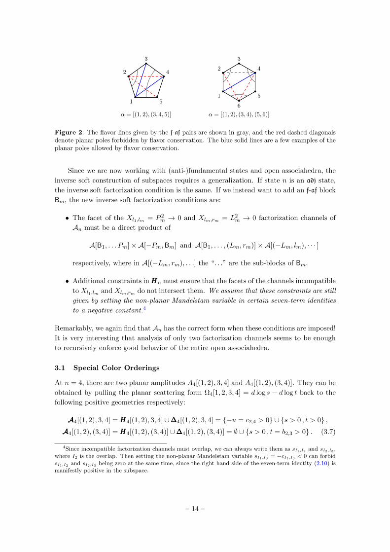
α = [(1, 2), (3, 4, 5)]

1

2

3

4

5

6

α = [(1, 2), (3, 4), (5, 6)]

Figure 2. The flavor lines given by the f-af pairs are shown in gray, and the red dashed diagonalsdenote planar poles forbidden by flavor conservation. The blue solid lines are a few examples of theplanar poles allowed by flavor conservation.

Since we are now working with (anti-)fundamental states and open associahedra, the

inverse soft construction of subspaces requires a generalization. If state n is an adj state,

the inverse soft factorization condition is the same. If we instead want to add an f-af block

Bm, the new inverse soft factorization conditions are:

• The facet of the Xl1,lm = P 2m → 0 and Xlm,rm = L2

m → 0 factorization channels of

An must be a direct product of

A[B1, . . . Pm]×A[−Pm,Bm] and A[B1, . . . , (Lm, rm)]×A[(−Lm, lm), · · · ]

respectively, where in A[(−Lm, rm), . . .] the “. . .” are the sub-blocks of Bm.

• Additional constraints inHHHn must ensure that the facets of the channels incompatible

to Xl1,lm and Xlm,rm do not intersect them. We assume that these constraints are still

given by setting the non-planar Mandelstam variable in certain seven-term identities

to a negative constant.4

Remarkably, we again find that An has the correct form when these conditions are imposed!

It is very interesting that analysis of only two factorization channels seems to be enough

to recursively enforce good behavior of the entire open associahedra.

3.1 Special Color Orderings

At n = 4, there are two planar amplitudes A4[(1, 2), 3, 4] and A4[(1, 2), (3, 4)]. They can be

obtained by pulling the planar scattering form Ω4[1, 2, 3, 4] = d log s − d log t back to the

following positive geometries respectively:

AAA4[(1, 2), 3, 4] = HHH4[(1, 2), 3, 4] ∪∆∆∆4[(1, 2), 3, 4] = −u = c2,4 > 0 ∪ s > 0 , t > 0 ,AAA4[(1, 2), (3, 4)] = HHH4[(1, 2), (3, 4)] ∪∆∆∆4[(1, 2), (3, 4)] = ∅ ∪ s > 0 , t = b2,3 > 0 . (3.7)

4Since incompatible factorization channels must overlap, we can always write them as sI1,I2 and sI2,I3 ,where I2 is the overlap. Then setting the non-planar Mandelstam variable sI1,I3 = −cI1,I3 < 0 can forbidsI1,I2 and sI2,I3 being zero at the same time, since the right hand side of the seven-term identity (2.10) ismanifestly positive in the subspace.

– 14 –

The former is the same as the bi-adjoint case, while for the latter, we have t = const in

∆∆∆4[(1, 2), (3, 4)] as the flavor conservation forbids this channel. Since now the subspace ∆4

is already one dimensional, no more constraints are needed so HHH4 = ∅ and H4 is simply

the full two-dimensional plane R2 spanned by s and t. One can easily show that indeed,

Ω4[1, 2, 3, 4]∣∣∣A4[(1,2),3,4]

=(1

s+

1

t

)ds = A4[(1, 2), 3, 4]ds ,

Ω4[1, 2, 3, 4]∣∣∣A4[(1,2),(3,4)]

=ds

s= A4[(1, 2), (3, 4)]ds . (3.8)

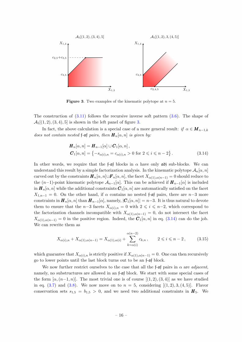
Starting from eq. (3.7), we show that certain five-point subspaces can be obtained by

an inverse soft construction. While the subspace for the ordering [(1, 2), 3, 4, 5] is given

in eq. (3.6), we begin with [(1, 2), (3, 4), 5] as an example. Adding the adj particle 5 to

[(1, 2), (3, 4)] does not lead to any new flavor constraints, so we have

FFF 5[(1, 2), (3, 4), 5] = FFF 4[(1, 2), (3, 4)] = s2,3 = b2,3 > 0 , (3.9)

which makes ∆5[(1, 2), (3, 4), 5] a four dimensional subspace. We thus need two more

constraints in HHH5 to make A5 a two dimensional kinematic polytope in which the facet

X1,4 = 0 gives the previous four-point sub-geometry X1,3 > 0. Thus the two additional

constraints need to ensure that the facets X2,5 = 0 and X3,5 = 0 do not intersect X1,4 = 0

in the positive region. One can check that the following two constraints can do the job:

−c2,5 +X2,5 +X1,3 = X3,5 , −c3,5 +X3,5 +X1,4 = X1,3 . (3.10)

Now we have already reduced the dimension of the subspace to two, no more constraints

can be added. We thus have

HHH5[(1, 2), (3, 4), 5] = −s2,5 = c2,5 > 0,−s3,5 = c3,5 > 0= HHH4[(1, 2), (3, 4)] ∪CCC1[(1, 2), (3, 4), 5] . (3.11)

Since HHH4[(1, 2), (3, 4)] = ∅, the set CCC1[(1, 2), (3, 4), 5] is just the right hand side of the first

line. If we choose X1,3 and X1,4 as the basis, the kinematic polytope A5[(1, 2), (3, 4), 5] is

bounded by the following inequalities:

X1,3 > 0 , X2,5 = −X1,4 + c2,5 + c3,5 > 0 ,

X1,4 > 0 , X3,5 = X1,3 −X1,4 + c3,5 > 0 . (3.12)

One can verify that by pulling the five-point planar scattering form (2.5) back to the

subspace A5[(1, 2), (3, 4), 5], we get the correct amplitude:

Ω5[1, 2, 3, 4, 5]∣∣∣A5[(1,2),(3,4),5]

=( 1

X1,3X1,4+

1

X1,3X3,5+

1

X2,5X3,5

)d2X

= A5[(1, 2), (3, 4), 5] d2X . (3.13)

– 15 –

A5[(1, 2), (3, 4), 5]

X1,3

X1,4

c2,5+c3,5

c3,5

A5[(1, 2), 3, (4, 5)]

X1,3

X1,4

c2,4,5

c3,5

Figure 3. Two examples of the kinematic polytope at n = 5.

The construction of (3.11) follows the recursive inverse soft pattern (3.6). The shape of

A5[(1, 2), (3, 4), 5] is shown in the left panel of figure 3.

In fact, the above calculation is a special case of a more general result: if α ∈MMMn−1,k

does not contain nested f-af pairs, then HHHn[α, n] is given by:

HHHn[α, n] = HHHn−1[α] ∪CCC1[α, n] ,

CCC1[α, n] =−sα(i),n = cα(i),n > 0 for 2 6 i 6 n− 2

. (3.14)

In other words, we require that the f-af blocks in α have only adj sub-blocks. We can

understand this result by a simple factorization analysis. In the kinematic polytopeAn[α, n]

carved out by the constraintsHHHn[α, n]∪FFFn[α, n], the facet Xα(1),α(n−1) = 0 should reduce to

the (n−1)-point kinematic polytope An−1[α]. This can be achieved if HHHn−1[α] is included

inHHHn[α, n] while the additional constraints CCC1[α, n] are automatically satisfied on the facet

X1,n−1 = 0. On the other hand, if α contains no nested f-af pairs, there are n−3 more

constraints inHHHn[α, n] thanHHHn−1[α], namely, |CCC1[α, n]| = n−3. It is thus natural to devote

them to ensure that the n−3 facets Xα(i),n = 0 with 2 6 i 6 n−2, which correspond to

the factorization channels incompatible with Xα(1),α(n−1) = 0, do not intersect the facet

Xα(1),α(n−1) = 0 in the positive region. Indeed, the CCC1[α, n] in eq. (3.14) can do the job.

We can rewrite them as

Xα(i),n +Xα(1),α(n−1) = Xα(1),α(i) +

α(n−2)∑k=α(i)

ck,n , 2 6 i 6 n− 2 , (3.15)

which guarantee thatXα(i),n is strictly positive ifXα(1),α(n−1) = 0. One can then recursively

go to lower points until the last block turns out to be an f-af block.

We now further restrict ourselves to the case that all the f-af pairs in α are adjacent,

namely, no substructures are allowed in an f-af block. We start with some special cases of

the form [α, (n−1, n)]. The most trivial one is of course [(1, 2), (3, 4)] as we have studied

in eq. (3.7) and (3.8). We now move on to n = 5, considering [(1, 2), 3, (4, 5)]. Flavor

conservation sets s1,5 = b1,5 > 0, and we need two additional constraints in HHH5. We

– 16 –

can obtain this ordering by gluing a three-point vertex [−q, (4, 5)] to [(1, 2), 3, q]. On

the facet X1,4 = 0 the subspace should return to that of [(1, 2), 3, q], which is given by

−s2,q = const. We thus get the first constraint −s2,q → −s2,4,5 = const for HHH5 from this

“inverse factorization” consideration. The second constraint needs to guarantee that the

facet X3,5 = 0 does not intersect X1,4 = 0, which can be achieved by −s3,5 = c3,5 > 0.

Therefore, we have

HHH5[(1, 2), 3, (4, 5)] = −s2,4,5 = c2,4,5 > 0,−s3,5 = c3,5 > 0FFF 5[(1, 2), 3, (4, 5)] = s1,5 = b1,5 > 0 . (3.16)

If we still choose X1,3, X3,5 as the basis, the kinematic polytope A5[(1, 2), 3, (4, 5)] is

bounded by the following inequalities:

X1,3 > 0 , X3,5 = X1,3 −X1,4 + c3,5 > 0 ,

X1,4 > 0 , X2,4 = X1,4 −X1,3 + c2,4,5 > 0 . (3.17)

It is then straightforward to check that the pullback of the form (2.5) indeed gives the

correct amplitude:

Ω5[1, 2, 3, 4, 5]∣∣∣A5[(1,2),3,(4,5)]

=( 1

X1,3X1,4+

1

X1,4X2,4+

1

X1,3X3,5

)d2X

= A5[(1, 2), 3, (4, 5)] d2X . (3.18)

The shape of A5[(1, 2), 3, (4, 5)] is shown in the right panel of figure 3.

We can generalize the above calculation to the following statement: if all the f-af pairs

are adjacent in α ∈MMMn−2,k, then HHHn[α, (n− 1, n)] is given by:

HHHn[α, (n−1, n)] = HHHn−1[α, q]∣∣∣sq,...→sn−1,n,...

∪CCC2[α, (n−1, n)]

= HHHn−2[α] ∪CCC1[α, (n−1, n)] ∪CCC2[α, (n−1, n)] . (3.19)

The second equality holds since we can write HHHn−1[α, q] = HHHn−2[α] ∪CCC1[α, q], and the q

only appears in CCC1. Thus the replacement sq,... → sn−1,n,... only affects CCC1:

CCC1[α, (n−1, n)] = CCC1[α, q]∣∣∣sq,...→sn−1,n,...

. (3.20)

It ensures that on the facet Xα(1),n−1 = q2 = 0, the constraints land back on HHHn−1[α, q].

To reach an (n−3)-dimensional kinematic polytope, a simple counting from eq. (3.3) shows

that we need |CCC2[α, (n−1, n)]| = n−k−2. The additional constraints should be auto-

matically satisfied on Xα(1),n−1 = 0. Therefore, we use them to ensure that the n−k−2

incompatible factorization channels at Xα(1),n−1 = 0,

Xα(i),n for each adj particle i or each f-af pair (i, i+ 1) with 3 6 i 6 n− 2, (3.21)

– 17 –

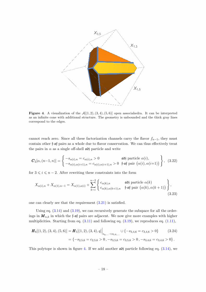
Figure 4. A visualization of the A[(1, 2), (3, 4), (5, 6)] open associahedra. It can be interpretedas an infinite cone with additional structure. The geometry is unbounded and the thick gray linescorrespond to the edges.

cannot reach zero. Since all these factorization channels carry the flavor fn−1, they must

contain other f-af pairs as a whole due to flavor conservation. We can thus effectively treat

the pairs in α as a single off-shell adj particle and write

CCC2[α, (n−1, n)] =

−sα(i),n = cα(i),n > 0 adj particle α(i),

−sα(i),α(i+1),n = cα(i),α(i+1),n > 0 f-af pair(α(i), α(i+1)

) , (3.22)

for 3 6 i 6 n− 2. After rewriting these constraints into the form

Xα(i),n +Xα(1),n−1 = Xα(1),α(i) +n−2∑k=i

cα(k),n adj particle α(k)

cα(k),α(k+1),n f-af pair(α(k), α(k + 1)

) ,(3.23)

one can clearly see that the requirement (3.21) is satisfied.

Using eq. (3.14) and (3.19), we can recursively generate the subspace for all the order-

ings in MMMn,k in which the f-af pairs are adjacent. We now give more examples with higher

multiplicities. Starting from eq. (3.11) and following eq. (3.19), we reproduces eq. (1.11),

HHH6[(1, 2), (3, 4), (5, 6)] = HHH5[(1, 2), (3, 4), q]∣∣∣sq,...→s5,6,...

∪ −s3,4,6 = c3,4,6 > 0 (3.24)

= −s2,5,6 = c2,5,6 > 0 ,−s3,5,6 = c3,5,6 > 0 ,−s3,4,6 = c3,4,6 > 0 .

This polytope is shown in figure 4. If we add another adj particle following eq. (3.14), we

– 18 –

get eq. (1.12),

HHH7[(1, 2), (3, 4), (5, 6), 7] = HHH6[(1, 2), (3, 4), (5, 6)] ∪ −si,7 = ci,7 > 0 for 2 6 i 6 5

=

s2,5,6 , s3,5,6 , s3,4,6 , s2,7 , s3,7 , s4,7 , s5,7

set to negative constants

. (3.25)

Finally, we can turn the last adj particle into a f-af pair (7, 8) using eq. (3.19), which leads

to eq. (1.13),

HHH8[(1, 2), (3, 4), (5, 6), (7, 8)]

= HHH7[(1, 2), (3, 4), (5, 6), q]∣∣∣sq,...→s7,8...

∪

s3,4,8 , s5,6,8

set to negative constants

(3.26)

=

s2,5,6 , s3,5,6 , s3,4,6 , s2,7,8 , s3,7,8 , s4,7,8 , s5,7,8 , s3,4,8 , s5,6,8

set to negative constants

.

We have checked up to n = 20 and ten adjacent f-af pairs that the algorithm indeed

generates the correct subspace.

3.2 Generic Recursive Construction

We now consider a generic α ∈MMMn,k, which can be put in the form of (2.25) by the enlarged

cyclic freedom. We can then read off the last block Bm and write

α = [B1,B2, . . . ,Bm−1,Bm] = [β,Bm] , where B1 = (l1, r1) or g1 . (3.27)

Suppose we already know the subspace constraints for the lower-point ordering β, our goal

is to obtain the constraints HHHn[α] through a recursion. The examples in the previous

subsection illustrate the idea for a more general construction.

We first study the case that Bm = n is a single adj particle and try to generalize the

inverse soft construction (3.14). When adding an adj particle n to an (n−1)-point ordering

β, we expect to write the result as

HHHn[α] = HHHn[β, n] = HHHn−1[β] ∪CCC1[β, n] , (3.28)

where HHHn−1[β] is the set of constraints for the kinematic polytope An−1[β]. Comparing

with eq. (3.14), the difference is that each block of β = [B1,B2, . . . ,Bm−1], except for

B1, may contain f-af sub-blocks as well as adj ones. On the facet Xl1,rm−1 = 0, the

constraints should reduce to HHHn−1[β], while those in CCC1[β, n] are automatically satisfied in

the positive region of the (n−1)-point kinematic subspace Kn−1 by the strict positivity of

the incompatible channels. Very crucially, these incompatible factorization channels are all

of the form Xli,n, Xri,n, XlI,n for each Bi and I ∈ sub[Bi], where lI is the first particle in

the sub-block I. For a single Bi, they are depicted in figure 5. In other words, the particle n

does not “see” any further substructures in I. The reason is that a planar propagator Xj,n

with j ∈ I ∈ sub[Bi] must cross the flavor line of (li, ri) and thus carry its flavor charge.

– 19 –

· · · · · · · · ·· · ·

li2 ri2 li3

ri3

li1

ri1

ri

li li+1

l1 rm−1

n

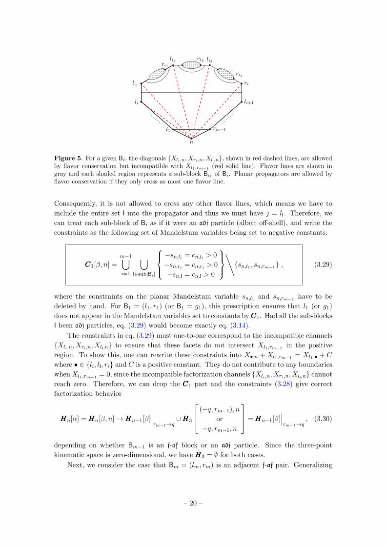
Figure 5. For a given Bi, the diagonals Xli,n, Xri,n, XlI,n, shown in red dashed lines, are allowedby flavor conservation but incompatible with Xl1,rm−1 (red solid line). Flavor lines are shown ingray and each shaded region represents a sub-block Bi` of Bi. Planar propagators are allowed byflavor conservation if they only cross as most one flavor line.

Consequently, it is not allowed to cross any other flavor lines, which means we have to

include the entire set I into the propagator and thus we must have j = lI. Therefore, we

can treat each sub-block of Bi as if it were an adj particle (albeit off-shell), and write the

constraints as the following set of Mandelstam variables being set to negative constants:

CCC1[β, n] =

m−1⋃i=1

⋃I∈sub[Bi]

−sn,li = cn,li > 0

−sn,ri = cn,ri > 0

−sn,I = cn,I > 0

∖sn,l1 , sn,rm−1 , (3.29)

where the constraints on the planar Mandelstam variable sn,l1 and sn,rm−1 have to be

deleted by hand. For B1 = (l1, r1) (or B1 = g1), this prescription ensures that l1 (or g1)

does not appear in the Mandelstam variables set to constants byCCC1. Had all the sub-blocks

I been adj particles, eq. (3.29) would become exactly eq. (3.14).

The constraints in eq. (3.29) must one-to-one correspond to the incompatible channels

Xli,n, Xri,n, XlI,n to ensure that these facets do not intersect Xl1,rm−1 in the positive

region. To show this, one can rewrite these constraints into X•,n + Xl1,rm−1 = Xl1,• + C

where • ∈ li, lI, ri and C is a positive constant. They do not contribute to any boundaries

when Xl1,rm−1 = 0, since the incompatible factorization channels Xli,n, Xri,n, XlI,n cannot

reach zero. Therefore, we can drop the CCC1 part and the constraints (3.28) give correct

factorization behavior

HHHn[α] = HHHn[β, n]→HHHn−1[β]∣∣∣rm−1→q

∪HHH3

(−q, rm−1), n

or

−q, rm−1, n

= HHHn−1[β]∣∣∣rm−1→q

, (3.30)

depending on whether Bm−1 is an f-af block or an adj particle. Since the three-point

kinematic space is zero-dimensional, we have HHH3 = ∅ for both cases.

Next, we consider the case that Bm = (lm, rm) is an adjacent f-af pair. Generalizing

– 20 –

from eq. (3.19), we expect the result to be

HHHn[α] = HHHn[β, (lm, rm)] = HHHn−2[β] ∪CCC1[β, (lm, rm)] ∪CCC2[β, (lm, rm)] , (3.31)

where HHHn−2[β] is the set of constraints for the kinematic polytope An−2[β]. Following the

same reasoning for eq. (3.20), we require that the constraints land back on HHHn−1[β, q] =

HHHn−2[β] ∪ CCC1[β, q] on the facet Xl1,lm = q2 = 0, which naturally leads to the following

replacement on the CCC1 in eq. (3.29):

CCC1[β, (lm, rm)] = CCC1[β, q]∣∣∣sq,...→slm,rm,...

. (3.32)

The constraints CCC2, on the other hand, have to be automatically satisfied when Xl1,lm = 0

due to the positivity of incompatible factorization channels Xli,rm with 2 6 i 6 m−1.

Again, flavor conservation requires that if Xj,rm with j ∈ Bi is an admissible planar prop-

agator, we must have j = li since Xj,rm already carries the flavor of the pair (lm, rm). In

other words, the particle rm only “sees” other blocks Bi as a single off-shell adj particle.

This leads to the generalization from eq. (3.22):

CCC2[β, (lm, rm)] =m−1⋃i=2

−sBi,rm = cBi,rm > 0 . (3.33)

We note that the leg lm does not appear in the Mandelstam variables set to constants byCCC2.

There are m−2 constraints in CCC2, which equals to the number of incompatible channels

Xli,rm. If all the Bi’s are either adjacent f-af pairs or adj particles, these constraints

reduce to eq. (3.22). By rewriting eq. (3.33) as

Xli,rm +Xl1,lm = Xl1,li +m−1∑k=i

(Xlk,lk+1

+ cBk,rm), 2 6 i 6 m− 1 , (3.34)

one can easily see that when Xl1,lm = 0, they do not carve out any boundary in the

positive region of the kinematic space Kn−2 since Xli,rm cannot reach zero, such that they

can simply be dropped. Therefore, we have proved that the constraints (3.31) have the

correct factorization behavior at Xl1,lm = q2 = 0,

HHHn[α] = HHHn[β, (lm, rm)]→HHHn−1[β, q] ∪HHH3[−q, (lm, rm)] = HHHn−1[β, q] , (3.35)

where we have used HHH3 = ∅.

We now generalize eq. (3.31) and consider Bm be an f-af block with substructures

Bm = (lm,Bm1 , . . . ,Bms , rm). Similar to the previous special cases, we can obtain a recur-

sive construction by studying the factorization involving the last block. We first consider

– 21 –

Xlm,rm = L2m = 0, on which the amplitude should factorize as

An[α] = An[β,Bm] −→ AL[β, (Lm, rm)]1

Xlm,rm

AR[(−Lm, lm),Bm1 , . . . ,Bms ] , (3.36)

where Lm satisfies (Lm + rm)2 = sBm = Xl1,lm . We thus require that the constraints

HHHn[α] reduce to those for AL and AR on the facet Xlm,rm = 0. It is natural to include the

subspace constraints for the left and right sub-amplitudes into HHHn[α] and write

HHHn[α] = HHHn[β,Bm] = HHHn−|Bm|+2[β, (Lm, rm)] ∪CCC3[β,Bm]

∪HHH |Bm|[(−Lm, lm),Bm1 , . . . ,Bms ] . (3.37)

While the first and last piece of HHHn[α] are defined recursively, the CCC3 part contains the

constraints that automatically drop out when Xlm,rm = 0 due to the strict positivity of

the incompatible channels Xli,lI with 1 6 i 6 m−1 and I ∈ sub[Bm]. These incompatible

channels are shown in the left panel of figure 6. The number of constraints in CCC3 should

equal to the number of these incompatible channels.

On the other hand, we can write the recursion (3.37) into a form that better fits to

the factorization channel Xl1,lm = P 2m = 0, on which the amplitude behaves as

An[β,Bm]→ AL[β, Pm]1

Xl1,lm

AR[−Pm,Bm] . (3.38)

Starting from eq. (3.37), we use eq. (3.31) to further expand HHHn−|Bm|+2[β, (Lm, rm)],

HHHn−|Bm|+2[β, (Lm, rm)] = HHHn−|Bm|[β] ∪CCC1[β, (Lm, rm)] ∪CCC2[β, (Lm, rm)] . (3.39)

Using (Lm + rm)2 = P 2m, we can rewrite the CCC1 part as

CCC1[β, (Lm, rm)] = CCC1[β, (Lm, rm)]∣∣∣sLm,rm,...→sPm,...

= CCC1[β, Pm] , (3.40)

such that the combination HHHn−|Bm|[β] ∪CCC1[β, (Lm, rm)] becomes

HHHn−|Bm|[β] ∪CCC1[β, (Lm, rm)] = HHHn−|Bm|[β] ∪CCC1[β, Pm] = HHHn−|Bm|+1[β, Pm] . (3.41)

The amplitudeAR[−Pm,Bm] is given byHHH |Bm|+1[−Pm,Bm]. By using recursively eq. (3.37),

we can write it as

HHH |Bm|+1[−Pm,Bm] = CCC3[−Pm,Bm] ∪HHH |Bm|[(−Lm, lm),Bm1 , . . . ,Bms ] . (3.42)

whereCCC3[−Pm,Bm] must be a subset ofCCC3[β,Bm] that have support in K|Bm|+1. Therefore,

it consists of the constraints that automatically drop out when Xlm,rm = 0 due to the strict

positivity of Xl1,lI, since these channels are incompatible to Xlm,rm but live in K|Bm|+1.

– 22 –

· · ·· · ·

li ri

lm2rm2

lm1

rm1

lm

rm

l1

· · ·· · ·

li ri

lm2rm2

lm1

rm1

lm

rm

l1

Figure 6. Left: The diagonals of the form Xli,lI with I ∈ sub[Bm] and 2 6 i 6 m−1 are shown inred dashed lines. The diagonals Xl1,lI are shown in blue dashed lines. Both of them are allowed byflavor conservation but incompatible to Xlm,rm (red solid line). Right: Xli,lI with 2 6 i 6 m−1(red dashed lines) are also incompatible to Xl1,lm (red solid line). The diagonals Xli,rm (bluedashed line) are incompatible to Xl1,lm but not Xlm,rm ,

We can thus divide CCC3 into two parts,

CCC3[β,Bm] = CCCa3[−Pm,Bm] ∪CCCb3[β,Bm] , (3.43)

where CCC3[−Pm,Bm] = CCCa3[−Pm,Bm] and CCCb3[−Pm,Bm] = ∅. The constraints in CCCb3 auto-

matically drop out at both Xlm,rm = 0 and Xl1,lm = 0 due to the strict positivity of Xli,lIwith 2 6 i 6 m−1, while those in CCCa3 only drop out at the first factorization channel.

The joint effect of eq. (3.39) to (3.43) rearranges the recursion (3.37) into the following

equivalent form,

HHHn[β,Bm] = HHHn−|Bm|+1[β, Pm] ∪CCC2[β, (Lm, rm)] ∪CCCb3[β,Bm]

∪HHH |Bm|+1[−Pm,Bm] , (3.44)

where both CCC2 and CCCb3 drop out automatically when Xl1,lm = 0.

We next show that the following definitions of CCCa3 and CCCb3 guarantee the correct fac-

torization behavior at both Xlm,rm = 0 and Xl1,lm = 0,

CCCa3[−Pm,Bm] = −slm,rm = clm,rm > 0⋃

I∈sub[Bm]\Bms

−sI,rm = cI,rm > 0 ,

CCCb3[β,Bm] =

m−1⋃i=2

⋃I∈sub[Bm]

−sBi,I = cBi,I > 0 . (3.45)

Together with eq. (3.31), this completes the generic recursive construction (3.37). To show

– 23 –

that the CCC3 part indeed drops out when Xlm,rm = 0, we first rewrite them into

CCCa3 : Xl1,lI +Xlm,rm = XlI,rm +Xl1,lm +∑

lm6J<I

(cJ,rm +XlJ,lJ+1

), (3.46a)

CCCb3 : Xli,lI +Xlm,rm = Xlm,lI +Xli,rm +

m−1∑j=i

∑I6J6Bms

(cBj ,J +Xlj ,lj+1

+XlJ,lJ+1

), (3.46b)

where J+1 denotes the sub-block coming right after J and lJ+1 its first particle. If J = Bmsis the last sub-block, then lJ+1 := rm. In both equations, we have I ∈ sub[Bm]. The

summation in eq. (3.46a) is over all the sub-blocks before I, including lm. In eq. (3.46b),

we have 2 6 i 6 m−1, and the second summation is over all the sub-blocks between I and

the last sub-block Bms . At Xlm,rm = L2m = 0, neither eq. (3.46a) nor (3.46b) impose any

boundaries in the positive kinematic subspace since Xl1,lI and Xli,lI cannot reach zero. We

can thus drop the CCC3 part and arrive at the desired factorization behavior

HHHn[α]Xlm,rm=0−−−−−−→HHHL

n−|Bm|+2[β, (Lm, rm)] ∪HHHR|Bm|[(−Lm, lm),Bm1 , . . . ,Bms ] , (3.47)

where HHHL and HHHR only depend on the left and right kinematic subspace respectively. This

implies that the facet Xlm,rm = 0 of the polytope A is a direct product of AL and AR. The

canonical form thus factorizes as Ω(A)→ Ω(AL)∧Ω(AR) and the amplitude as eq. (3.36).

Similarly, to show that in eq. (3.44) the constraints in CCC2 and CCCb3 drop out automati-

cally when Xl1,lm = 0, we rewrite them as

CCC2 : Xli,rm +Xl1,lm = Xl1,li +Xlm,rm +

m−1∑j=i

(cBj ,rm +Xlj ,lj+1

), (3.48a)

CCCb3 : Xli,lI +Xl1,lm = Xlm,lI +Xl1,li +m−1∑j=1

(cBj ,rm +Xlj ,lj+1

)+

m−1∑j=i

∑I6J6Bms

(cBj ,J +Xlj ,lj+1

+XlJ,lJ+1

), (3.48b)

where 2 6 i 6 m−1 and I ∈ sub[Bm]. When Xl1,lm = 0, clearly Xli,rm and Xli,lI cannot

reach zero such that they do not give rise to any constraints. These incompatible channels

are also given in figure 6. Therefore, we get

HHHn[β,Bm]Xl1,lm=0−−−−−−→HHHL

n−|Bm|+1[β, Pm] ∪HHHR|Bm|+1[−Pm,Bm] , (3.49)

which is the desired factorization behavior that leads to a direct product geometry AL×AR

on the facet Xl1,lm = 0 of A.

We close this section by the explicit example of constructing the subspace constraints

for α = [(1, 2), (3, (4, 5), 6, 7), (8, 9, 10, 11)]. Since the last block (8, 9, 10, 11) is an f-af block

– 24 –

with substructures, we use eq. (3.37) to write

HHH11[β, (8, 9, 10, 11)] = HHH9[β, (P8,9,10, 11)] ∪CCC3[β, (8, 9, 10, 11)] ∪HHH4[(−P8,9,10, 8), 9, 10] ,

(3.50)

where β = [(1, 2), (3, (4, 5), 6, 7)]. The CCC3 part is given by eq. (3.45):

CCC3[β, (8, 9, 10, 11)] =

s8,11, s9,11, s3,4,5,6,7,9, s3,4,5,6,7,10

set to negative constants

, (3.51)

where the constraints on s8,11 and s9,11 come from CCCa3 and the rest from CCCb3. Using

eq. (3.31), we can write HHH9[β, (P8,9,10, 11)] as

HHH9[β, (P8,9,10, 11)] = HHH7[β] ∪CCC1[β, (P8,9,10, 11)] ∪CCC2[β, (P8,9,10, 11)] , (3.52)

where CCC1 and CCC2 are give by

CCC1[β, (P8,9,10, 11)] =

s2,8,9,10,11, s3,8,9,10,11, s4,5,8,9,10,11, s6,8,9,10,11

set to negative constants

,

CCC2[β, (P8,9,10, 11)] = s3,4,5,6,7,11 set to negative constant . (3.53)

Applying eq. (3.37) to HHH7[β] and HHH4[(−P8,9,10, 8), 9, 10], we get

HHH7[(1, 2), (3, (4, 5), 6, 7)] =

s3,6, s4,6, s3,7, s4,5,7

set to negative constants

,

HHH4[(−P8,9,10, 8), 9, 10] = s8,10 set to negative constant , (3.54)

where we have used eq. (3.28), or for this case equivalently eq. (3.14), to obtain HHH5.

Thus HHH11[(1, 2), (3, (4, 5), 6, 7), (8, 9, 10, 11)] is given by the union of all the constraints in

eq. (3.51), (3.53) and (3.54). The result agrees with eq. (1.14).

3.3 Remarks

We have checked up to n = 20 and a variety of block structures that if we pull-back

the planar scattering form Ωn[α] to the polytope An[α] given by the constraints AAAn[α] =

HHHn[α]∪∆∆∆n[α], where HHHn[α] is constructed from eq. (3.37) and ∆∆∆n[α] is the union of PPPn[α]

and FFFn[α] given in eq. (3.1), we get the correct amplitude,

Ωn[α]∣∣∣An[α]

= An[α]dn−3X . (3.55)

There are several interesting features in this open kinematic polytope that do not appear

in the bi-adjoint case. Although the facet geometry of Xlm,rm = 0 and Xl1,lm = 0 is

by construction a direct product of lower-dimensional polytopes carved out by the same

process as eq. (3.37), it is generally not true for other facets. When restricted to a generic

– 25 –

facet Xi,j = 0, we actually have

An[α]∣∣∣Xi,j=0

∼= AL[αL; a] nAR[αR] . (3.56)

While AR[αR] is given by eq. (3.37), AL[αL; a] is deformed by some linear combinations

of the planar Mandelstam variables in the left kinematic subspace, where a is a formal

collection of the deformation parameters. They change the shape of the polytope but leave

the expression of the canonical form unchanged after pull-back,

Ω[αL]∣∣∣A[αL;a]

= AL[αL]dn−3X . (3.57)

In appendix A, we will present a special class of such deformations on HHHn[α]. Moreover,

the facet geometry is a semi-direct product “n” between AL[αL; a] and AR[αR]: the c

constants in the constraints for AL[αL; a] receive a linear shift by the planar variables in

AR. The canonical form still factorizes nicely despite this shift,

ResXi,j=0Ωn[α,An] = Ωn[α,An|Xi,j=0] = Ωn[α,AL nAR] = Ω[αL,AL] ∧ Ω[αR,AR] ,

(3.58)

since the top form Ω[αR,AR] removes all the linear shifts in the c constants. We will give a

few concrete factorization examples that manifest these features in appendix B, and leave

the detailed factorization analysis to a future work.

4 “Color is Kinematics” for (Anti-)Fundamental States

We now turn to the positive geometry interpretation of full, color-dressed amplitudes with

(a)f states in more generic theories, not just partial amplitudes for scalar theories. We find

a natural extension of the “color is kinematics” philosophy of [1] to (anti-)fundamental am-

plitudes. In section 4.1, we first discuss a natural generalization of small kinematic space for

(anti-)fundamental scattering amplitudes which is necessary for (anti-)fundamental color-

kinematics duality. In section 4.2, we show how the duality between differentials forms

in kinematic space and color factors extends to (anti-)fundamental scattering forms. In

section 4.3, we focus on connections between BCJ numerator relations and projectivity for

(anti-)fundamental scattering forms. In section 4.4, we show how Melia decomposition is

dual to pulling back the scattering form to a specific sub-space, HTn [α]. Interestingly, the

k > 1 planar scattering form does not need to be a top-form like in the bi-adjoint case.

Since we will be dealing with (a)f states without a definite ordering, we introduce a

minor notation change from section 3. When referring to (a)f states, we will use capital

letters, where an underline (bar) indicates a f (af) state.

4.1 (Anti-)Fundamental Small Kinematic Space

We now define (anti-)fundamental kinematic space, Kkn. We start with big kinematic

space, K?n, which is the same for (anti-)fundamental and adjoint amplitudes. Big kinematic

– 26 –

I1 I2

I3I4

I1 I4

I2I3

I1 I3

I4I2

S = sI1I2 T = sI2I3 U = sI1I3

gS gT gU

Figure 7. A four-set partition I1 t I2 t I3 t I4 of the external labels and the three correspondingchannels. The three graphs gS , gT , gU are identical except for a 4-point subgraph. This is the sameas figure 1, but reproduced here for the reader’s convenience.

space is defined as a vector space spanned by SI variables, which are indexed by subsets,

I ⊂ 1, 2, . . . , n, and obey

• SI = SI where I is the complement of I,

• SI = 0 for |I| = 0, 1, n− 1, n.

The dimension of big kinematic space is

dim(K?n) = 2n−1 − n− 1 . (4.1)

As reviewed in section 2.2, the reduction to small kinematic space for k = 0 is done by

imposing the seven-term identity on all four-point sub-graphs.

For adjoint amplitudes, one can show that upon imposing the seven-term identity on

all sub-graphs, any variable sI can be written as a sum of si,j , which can be identified as

Mandelstam variables. Kk=0n is therefore spanned by Mandelstam variables, si,j , implying

that the seven-term identity is equivalent to imposing momentum conservation and that

the dimension of the space is

dim(Kk=0n ) =

n(n− 3)

2. (4.2)

The process of reducing from K?n to Kkn when k 6= 0, 1 is slightly modified. As in section 3,

internal propagators which violate flavor conservation are truncated from the vector space,

which leads to the (anti-)fundamental big kinematic space (Kkn)?,

SI = bI , if ϑI = 0 . (4.3)

To further reach the (anti-)fundamental small kinematic space Kkn, the seven-term identity

is then imposed on all sub-graphs except those where all Ii correspond to (a)f states,

SI1,I2 + SI2,I3 + SI1,I3 = SI1 + SI2 + SI3 + SI4 . (4.4)

– 27 –

This mirrors the color structure of tree graphs with (anti-)fundamental states, as visualized

in figure 8. We can interpret this generalization of kinematic space as a natural abstracti-

fication of momentum conservation where the seven-term identity is treated as fundamen-

tal. Due to the truncation procedure and fewer number of relations between remaining

SI , (anti-)fundamental small kinematic space has more non-trivial combinatorial structure

than adjoint small kinematic space. For example, the dimension of (anti-)fundamental

small kinematic space is

dim(Kkn) =n(n− 3)

2− k(k − 1)

2. (4.5)

Eq. (4.5) is derived in appendix C. In the small kinematic space, we identify SI with the

Mandelstam variable sI for each I. Furthermore, the two-particle Mandelstam variables

si,j do not always provide a complete basis for Kkn after the truncation of those forbidden by

the flavor structure. To see this, consider amplitudes with only (anti-)fundamental external

states. There are only k Mandelstam variables not forbidden by flavor conservation, which

is smaller than the dimension of the space for k > 3. Instead, a more natural basis is

the planar variables of some ordering, α, where all f-af pairs are adjacent. The number of

planar propagators for such orderings matches eq. (4.5).

As a simple example, consider the four-point amplitude M[A, A,B, B]. Big kinematic

space is the same as the adjoint case:

K?n = sA,A, sA,B, sA,B . (4.6)

To reduce to small kinematic space, the propagators forbidden by flavor conservation,

sA,B and sA,B, are truncated from the spectrum. Since the only possible four-point sub-

graph corresponds to four external (a)f states, there are no seven-term identities to impose.

Therefore, (ant-)fundamental small kinematic space is

Kk=2n=4 = sA,A = (Kk=2

n=4)? . (4.7)

Note that the dimension of Kk=2n=4 matches eq. (4.5).

Now consider the amplitude M[A, A,B, B, C, C]. To find small kinematic space, all

forbidden propagators are first truncated from the spectrum, leaving:

(Kk=3n=6)? =

SAA , SBB, SCC , SABB , SBCC , SCAA , SABB , SBCC , SCAA

(4.8)

The seven-term identity is then imposed on all valid four-point sub-graphs, of which there

are only three:

SI1,I2 + SI2,I3 + SI1,I3 = SI1 + SI2 + SI3 + SI4 ,

with I1 = A, I2 = A, I3 = B, B, I4 = C, C(A↔ B ↔ C) .

(4.9)

The (anti-)fundamental small kinematic space is therefore six dimensional, which again

– 28 –

+ + = 0

(a) Color algebra in the adjoint representation.

+ + = 0

(b) Color algebra in the fundamental representation that obeys a Jacobi-like identity.

+ 6= 0

(c) Color algebra in the fundamental representation that does not obey a Jacobi-like identity.

Figure 8. Graphic representations of the color algebra for theories with (anti-)fundamental andadjoint states.

matches eq. (4.5) for k = 3, n = 6.

4.2 Duality between Differential Forms and Color Factors

The notion of a scattering form, which corresponds to the full, color-dressed amplitude,

has a natural application to amplitudes with (a)f states. Without losing any information,

we can pullback the scattering form (2.8) to the (anti-)fundamental big/small kinematic

space, which leads to the (anti-)fundamental scattering form

Ωkn[N ] =

∑g∈Γn

N(g|αg)W (g|αg)∏I∈g

ϑIsI

, (4.10)

where the summation is effectively over all cubic graphs that respect flavor conservation

since ϑI defined in eq. (2.23) kills those graphs that violate it, and W is a differential form

W (g|αg) = sign(g|αg)∧g∈I

dsI . (4.11)

Unlike the adjoint scattering forms, which live in Kk=0n , the (anti-)fundamental dlog forms

live in (anti-)fundamental small kinematic space, Kkn.

The duality between differential forms and color factors generalizes to (anti-)fundamental

scattering forms. In the (anti-)fundamental case, the color factor is a product of structure

– 29 –

constants and fundamental representation matrices. Relations between color factors arise

from both Jacobi and commutation identities

fabef cde + f bcefade + f caef bde = 0 ,

(T aT b)ij − (T bT a)ij − fabc(T c)ij = 0 .(4.12)

Unlike the adjoint case, the Jacobi-like identities for color factors in eq. (4.12) do not apply

to all four-point sub-graphs. When all external states are (a)f states, the color factors are

Cs ∝ (T a)i1i2(T a)i3i4 , Ct ∝ (T a)i1i4(T a)i3i2 , Cu = 0 , (4.13)

which clearly do not obey a Jacobi-like relation. The relation

C(gS |I1I2I3I4) + C(gT |I1I4I2I3) + C(gU |I1I3I4I2) = 0 , (4.14)

therefore applies to all four-point sub-graph except those where all Ii correspond to (a)f

states. We now argue that the set of identities in eq. (4.14) exactly mirror the seven-term

identity. Taking the differential of eq. (4.4) and repeating the argument in section 2.2, we

see that for any triplet of graphs corresponding to eq. (4.14):

(dsI1,I2 + dsI1,I3 + dsI1,I4) ∧n−4∧b=1

dsJb , (4.15)

where sJb denotes the propagators shared by the triplet of graphs. It follows that,

W (gS |I1I2I3I4) +W (gT |I1I4I2I3) +W (gU |I1I3I4I2) = 0 , (4.16)

only applies to desirable four-point sub-graphs and is therefore dual to eq. (4.14).

Consider the four-point amplitude M[AiAjBmBn] with two pairs of (anti-)fundamental

particles. Here, we explicitly display the (anti-)fundamental representation indices of the

particles. There is only a single Feynman diagram contribution, so there is only one color-

factor dual to a one-form:

Cs = (T a)ij(Ta)mn ↔ ds . (4.17)

There is no U -channel graph, because it is forbidden by flavor charge conservation.

Now consider the four-point amplitude M[AiAjφaφb] in which φa and φb are two adjoint

representation particles. There are three color factors dual to one forms:

Cs = fabc(T c)ij ↔ ds ,

Ct = (T bT a)ij ↔ dt ,

Cu = −(T aT b)ij ↔ du .

(4.18)

– 30 –

The duality holds because there exists a valid seven-term identity that leads to the linear

relation between the differentials,

ds+ dt+ du = 0 , (4.19)

which corresponds to the second line of eq. (4.12).

4.3 (Non-)Projectivity of the Scattering Form

In this sub-section, we connect projectivity of the (anti-)fundamental scattering without

flavor structure to generalized Jacobi identities for kinematic numerator factors.

We first consider the usual scattering form (2.8) in big kinematic space K?n. Projec-

tivity of a differential form is defined as the invariance under a local GL(1) transformation

SI → Λ(S)SI . Projectivity of the scattering form in K?n could be used to derive Jacobi

identities for kinematic numerator factors [1]. To see this, note that the Λ dependence of

the scattering form under a local GL(1) transformation is

[N(gS |I1I2I3I4) +N(gT |I1I4I2I3) +N(gU |I1I3I4I2)

]d log(Λ) ∧

(n−4∧b=1

d log(SJb)

)+ . . . ,

(4.20)

where SJb denote the (n−4) propagators shared by a triplet of graphs and the “. . .” denotes

the same expression for all other triplet. It is clear that the Λ-dependence only vanishes

if the kinematic numerators obey Jacobi identities. It is key that we are only considering

projectivity in big kinematic space, as the d log(sI) factors would be related by linear

relations in small kinematic space. Such linear relations could lead to cancellations between

triplets.

Unlike the adjoint case, the (anti-)fundamental scattering form (4.10) with k > 1

distinct flavor f-af pairs cannot be projective. This is obvious already at four-points. A

generic k = 2, n = 4 scattering form takes the form,

Ωk=2n=4[N ] = N(gS |AABB)d log(S) , (4.21)

which clearly cannot be invariant under a local GL(1) transform. However, if all (a)f states

transform in the same flavor representation, the scattering form is projective. Consider the

four-point example again, except now all states transform in the same flavor representation:

Ωnf=1,k=2n=4 [N ] = N(gS |AABB)d log(S) +N(gT |ABAB)d log(T ) . (4.22)

The f-af pairs A and B now have the same flavor so sAB is not forbidden by flavor conser-

vation. Under a local GL(1) transformation, the scattering form transforms as

Ωnf=1,k=2n=4 [N ]→ (N(gS |AABB) +N(gT |ABAB))d log(Λ) + Ω

nf=1,k=2n=4 [N ] . (4.23)

– 31 –

Therefore, the requirement that the scattering form is projective imposes that

N(gS |AABB) +N(gT |ABAB) = 0 . (4.24)

This relation generalizes to higher points, where projectivity of the nf = 1 scattering form

implies

N(gS |I1I2I3I4) +N(gT |I1I4I2I3) +N(gU |I1I3I4I2) = 0 , (4.25)

for all sub-graphs which do not violate charge conservation. For sub-graphs corresponding

to all f-af external states, the kinematic factor associated with the propagator that violates

charge conservation is simply zero and eq. (4.25) reduces to a two-term identity.

Eq. (4.25) is interesting for a number of reasons. For example, for sub-graphs cor-

responding to all f-af external states, eq. (4.25) does not correspond to any relationship

that color factors obey as eq. (4.14) does not apply to sub-graphs corresponding to all f-af

external states. Instead, we see that eq. (4.25) can be considered a natural generalization of

color-kinematics duality that emerges from requiring the scattering form to be projective.

These two-term identities were noted in [23], but not expanded on further as they were not

necessary for their double-copy prescription. In addition, the applicablity of eq. (4.25) to

ALL sub-graphs implies that the original KLT relations can be applied to nf = 1 (anti-

)fundamental amplitudes [24–26]. The only difference between nf = 1 (anti-)fundamental

amplitudes and adjoint amplitudes is that many of the kinematic numerator factors in the

(anti-)fundamental amplitudes are trivially zero due to violating charge conservation.

A natural extension of eq. (4.25) is studying what conditions the scattering form must

obey to be projective in Kkn. For the adjoint scattering form, projectivity in Kk=0n is equiv-

alent to BCJ relations.5 Importantly, while the numerator Jacobi identity implies BCJ

relations, BCJ relations do not imply the Jacobi numerator identity. In the language of

positive geometry, while projectivity in big kinematic space implies projecitivty in small

kinematic space, projectivity in small kinematic space does NOT imply projectivity in big

kinematic space. The corresponding generalizations of the Jacobi kinematic identity which

obey BCJ relations were explored in [28]. It would be interesting to see if there exists

a natural generalization of the BCJ identities for (anti-)fundamental amplitudes, which

would in turn provide a generalization of the two term identity.

4.4 Melia Decomposition Dual to Pullback

We now further explore the color-kinematics duality by examining how the Melia decom-

position of the amplitude is dual to pulling back the scattering form to an appropriate

subspace, HTn [α]. Unlike the adjoint case, this sub-space generally has higher dimension

than (n − 3), but the pulled-back scattering form only depends on the coordinates of the

(n − 3)-dimensional subspace, Hn[α]. We will simply state the qualitative results here,

leaving the technical details to Appendix D.

In the case of (anti-)fundamental color-dressed amplitudes, the color-dressed ampli-

5BCJ-like relations for QCD amplitudes are studied in [27].

– 32 –

tuded can be decomposed into a sum of partial amplitudes using eq. (4.12) and requiring

that the kinematic numerators, N(g|α), obey the same relations as their associated color

factors [20]. The Melia decomposition of the amplitude is

Mn[N ] =∑

σ∈Melia basis

C ′((1, 2), σ)M [N ; (1, 2), σ] , (4.26)

where the sum is over all valid Melia basis orderings. The color constants C ′((1, 2), σ) are

non-trivial color constants given explicitly in [20] and Mn[N ; (1, 2), σ] is the color-stripped

partial amplitude:

Mn[N ;α] =∑

α-planar g

N(g|αg)∏I∈g

ϑIsI

. (4.27)

For the dual scattering form, we claim that Melia decomposition of the partial amplitude

is dual to pulling back the scattering form to a specific subspace. The partial amplitude,

eq. (4.27), can be obtained by pulling back the scattering form, eq. (4.10), to a subspace

HTn [α],6 where

W (g|κ)|HTn [α] =

(−1)flip(κ,α)dV [α] if g is compatible with α

0 otherwise. (4.28)

where flip(κ, α) is the number of vertex flips that relates κ and α. Moreover, here κ can

be any ordering of external states, unlike α, for which the first two states must be a f-af

pair. Unlike the adjoint case, the (anti-)fundamental scattering form after the pullback is

not a top-form of HTn [α] but only depends on the coordinates of the (n−3)-dimensional

subspace Hn[α] ⊂ HTn [α]. The measure “dV [α]” is a volume form of Hn[α], not HT

n [α].

This phenomena is a direct consequence of the fact that the planar scattering form is not

a top-form of Kkn.

The pullback to HTn [α] can be understood as follows. We consider the planar scattering

form, Ω[N ;α],

Ω[N ;α] :=∑g∈Γ[α]

N(g|αg)W (g|αg)∏I∈g

ϑIsI, (4.29)

where Γ[α] ⊂ Γn is the set of all the graphs compatible with the planar ordering α. Ac-

cording to eq. (4.28), only the planar scattering form should survive upon pullback of the

full scattering form, eq. (3.37), to HTn [α]. However, unless all f-af pairs are adjacent in

α, the planar variables associated with Ω[N ;α] do not span Kkn. Therefore, since Ω[N ;α]

only depends on the coordinates of the planar variables, we can say that Ω[N ;α] only has

6We focus on Melia decomposition, and not color-trace decomposition, because the duality between colorfactors and differentials is applicable to theories transforming in any gauge group, such as Sp(N), and naivecolor trace decomposition is not. To see this, note that our derivation in the previous section only relied onthe definition of the structure constants and commutation relations. We did not use any properties uniqueto SU(N) or U(N) groups.

– 33 –

support on the affine subspace Kkn[α] in Kkn.7 We denote the orthogonal complement to

Kkn[α] as Dkn[α]:

Dkn[α] = (Kkn[α])⊥ . (4.30)

The full relationship between Dkn[α], Kkn[α], and Kkn is

Kkn = Kkn[α]⊗Dkn[α] . (4.31)

The planar scattering form only has support in Kkn[α], but the full scattering form Ω(n−3)[N ]

has support in Dkn[α] as well. Based on eq. (4.31), we can decompose HTn [α] as

HTn [α] = Hn[α]⊗HA

n [α], Hn[α] ⊂ Kkn[α], HAn [α] ⊂ Dkn[α] , (4.32)

where dim(Hn[α]) = (n − 3) and dim(HAn [α]) > 0 for the auxiliary space HA

n [α]. The

space Hn[α] is simply given by the restrictions HHHn[α] in eq. (3.37) from section 3.2. This

automatically validates the first line of eq. (4.28) by construction. However, the restrictions

from HHHn[α] are not enough to get rid of all incompatible graphs for generic orderings with

k > 3. This is unsurprising as the incompatible graphs for generic α have support in

Dkn[α] as well as Kkn[α], so additional restrictions from HHHAn [α] are necessary to remove these

unwanted contributions. Due to the complexity of HHHAn [α], we leave computational results

to appendix D, where a closed form for HHHAn [α] is provided in eq. (D.11).

5 Conclusion

In this paper we initiate the study of positive geometry and scattering forms for amplitudes

with matter particles, i.e. particles flavored in (anti-)fundamental representations. The

original paper [1], which treats scattering amplitudes as differential forms in kinematic

space, has focused on amplitudes with particles purely in adjoint representation; here we

pinpoint the new ingredients to include matter particles in this geometric picture. As a

toy model, we find that a class of the so-called open associahedra, i.e. associahedra with

certain faces sent to infinity, underpin all tree-level amplitudes of the bi-color φ3 scalar

theory, where the bi-adjoint scalars and bi-fundamental ones play the role of “gluons” and

“quarks”, respectively. For any flavor assignment and a given planar ordering, we obtain an

open associahedron which is determined by a (n−3)-dim subspace in the kinematic space;

the canonical form then gives the corresponding amplitudes, with forbidden poles sent to

infinity. Moreover, we discuss “color is kinematics”, i.e. the duality between color factors

and wedge-products for cubic diagrams now in the presence of matter particles, and the

projectivity of the scattering forms when there is only a single flavor.

There are many open questions suggested by our preliminary discussions. First, we

would like to study further the construction of subspaces for bi-color amplitudes, e.g.

how the inverse soft construction etc. can be generalized, and how to obtain other open

7Our construction of Kkn[α] is very similiar to the construction of the affine subsapce Y[Z] from generaltwistor space in section 9 of [3]. The planar coordinates that form a complete basis for Kkn[α] are analogousto the yiα that span the affine subspace Y[Z].

– 34 –

polytopes which are relevant for scattering amptlidues such as the Cayley polytopes [14,

15]. Moreover, it is straightforward to generalize our construction to off-diagonal bi-color

amplitudes, m[α|β] for α 6= β; the latter is given by the intersection of the diagonal cases

with α and β ordering [12, 13]. We similarly conjecture that the bi-color amplitude can

be obtained as the volume of intersection of the corresponding dual open associahedra. A

related open question is how to obtain a inverse matrix which can be used as the KLT

matrix for QCD amplitudes [8, 9].

An alternative direction is considering different triangulations of the canonical forms

of open associahedra, which would in turn yield recursion relations for bi-color theory. Due

to facets at infinity, the recursions given in [1, 5] initially seem somewhat impractical for

efficient calculations. It would be interesting to see if the triangulation in [29, 30] could be

generalized to open associahedra, yielding a BCFW-like recursion for bi-color amplitudes.

It is possible that the inverse soft construction of the amplitude would be intimately tied

to any such recursion. Another approach is considering triangulations of the dual polytope

that are not trivially equivalent to the Feynman diagram expansion.

The construction we proposed reveal rich structures underlying such positive geometry

which deserve further investigations by themselves. In [31] the ABHY associahedron is

generalized to polytopes for other finite-type cluster algebra, where the classical cases

correspond to bi-adjoint φ3 amplitudes through one loop. It would be interesting to extend

that construction to open cases with facets at infinity. We note that the factorization

channels used in our construction are similar to those for constructing mulit-quark color

decomposition [32].

Throughout the paper we have not discussed the worldsheet perspective (string theory

and CHY) for bi-color amplitudes and open associahedra. It is not difficult to come up

with CHY formulas for such amplitudes, and some of them coincide with CHY formulas

for Cayley polytopes [15]. However, for general case the one-to-one map from moduli

space to kinematic space and pushforward for scattering forms are still missing. The

proper framework to proceed is the stringy canonical forms of [33], and it would be highly

desirable to find such string-like integrals where the so-called Minkowski sum of Newton

polytopes gives an open associahedron. We remark that this new picture leads to new,

CHY-like formulas for bi-color amplitudes, and we leave it to future investigations.

Acknowledgments

We would like to thank Alfredo Guevara, Marios Hadjiantonis, Henrik Johansson, Cal-

lum R. T. Jones, Gregor Kalin, Alok Laddha, Stephen Naculich, Shruti Paranjape and

Jaroslav Trnka for inspiring discussions. AH would like to especially thank Henriette

Elvang for instrumental support and discussion early in the project. SH’s research is

supported in part by the Thousand Young Talents program, the Key Research Program

of Frontier Sciences of CAS under Grant No. QYZDBSSW-SYS014, Peng Huanwu center

under Grant No. 11747601 and National Natural Science Foundation of China under Grant

No. 11935013. FT is supported by the Knut and Alice Wallenberg Foundation under grant

KAW 2013.0235, and the Ragnar Soderberg Foundation (Swedish Foundations’ Starting

– 35 –

Grant). FT would also like to thank the hospitality of CAS key laboratory of theoretical

physics and Leinweber Center for Theoretical Physics at the University of Michigan.

A Possible Deformations on Constraints

The subspace constraints HHHn[α] in eq. (3.37) are all of the form −sA,C = cA,C > 0 with

non-adjacent sets A and C. However, we can introduce certain deformations to HHHn[α],

and thus the polytope, while keep the canonical form unchanged. In fact, certain facets of

the kinematic polytope given by HHHn[α] are characterized by deformed constraints. Thus

deformations are essential to understand generic factorization behavior of the polytope.

Here, we provide a special class of such deformations, and leave more generic discussions

to a following work [34].

For a given block Bi, we rewrite the constraints on sLj ,rj ,ri = sBj ,ri with j > i+2 in

favor of those on sBj ,Bi . These constraints come from the CCC1 part in the recursive process

when the block Bj is added. We first use the seven-term identity (2.10) to write

−sBi,Bj = −sBj ,ri +Xli,lj −Xri,lk +Xlj+1,ri −Xlj+1,li −Xli,li+1. (A.1)

With the help of the constraints on sBj ,li , sBj ,I | I ∈ sub[Bi] also generated in CCC1, the right

hand becomes

−sBi,Bj = cBj ,ri + cBj ,li +Xlj ,lj+1−Xli,li+1

+∑

I∈sub[Bi]

(cBj ,I +XlI,lI+1

+Xlj ,lj+1

)= cBj ,ri + cBj ,li + (di + 1)Xlj ,lj+1

−Xli,li+1+

∑I∈sub[Bi]

(cBj ,I +XlI,lI+1

), (A.2)

where di counts the number of sub-blocks in Bi. If I is the last sub-block, then lI+1 = ri.

The constraint (A.2) is completely equivalent to −sBj ,ri = cBj ,ri > 0. We can thus use the

former instead of the latter in HHHn[α] and the resultant polytope An[α] is unchanged. Now

suppose Bi actually contains a additional sub-blocks but all of which are taken soft, one

can check that we recover most of the constraints in HHHn[α] while the only trace of these

soft sub-blocks is in eq. (A.2): di gets shifted by a,

−sBi,Bj = cBj ,ri + cBj ,li + (di + a+ 1)Xlj ,lj+1−Xli,li+1

+∑

I∈sub[Bi]

(cBj ,I +XlI,lI+1

). (A.3)

If Bi = gi is an adj particle, then we can start with a generic block and take all the

sub-blocks, including the pair (li, ri), to be soft, which leads to a similar formula:

−sgi,Bj = cgi,Bj + aXlj ,lj+1. (A.4)

Switching back to the constraint on sBj ,ri amounts to cast the shift aXlj ,lj+1onto the

– 36 –

constant cBj ,ri for i+ 2 6 j 6 m:

HHHn[α; a] = HHHn[B1, . . . ,Bi, . . . ,Bm; a]

= HHHn[α]∣∣∣−sBj ,ri=cBj ,ri→−sBj ,ri=cBj ,ri+aXlj ,lj+1

for i+26j6m . (A.5)

We note that Bi = gi being an adj particle is also covered by the above replacement because

we identify li = ri = gi. If all the blocks are adj particles, these shifts vanish identically

since Xlj ,lj+1= 0 for all cases. For example, the constraints

HHH7[(1, 2), q, (5, 6), (7, 8)] =

s2,5,6, s5,6,8, sq,6, sq,8, s2,7,8, s5,7,8, sq,7,8

set to negative constants

(A.6)

allow the following deformation on sq,7,8 according to eq. (A.5),

HHH7[(1, 2), q, (5, 6), (7, 8); a] =

s2,5,6, s5,6,8, sq,6, sq,8, s2,7,8, s5,7,8

set to negative constants

∪ −sq,7,8 = cq,7,8 + aX1,7 . (A.7)

This deformation is relevant to the X3,5 = q2 = 0 facet of A8[(1, 2), (3, 4), (5, 6), (7, 8)], as

we will see in the next appendix.

We denote the polytope obtained fromHHHn[α; a] as An[α; a]. We have checked a variety

of examples to high enough multiplicity that the canonical form after the pullback has the

same expression,

Ωn[α]∣∣∣An[α]

= An[α]dn−3X , Ωn[α]∣∣∣An[α,a]

= An[α]dn−3X , (a > 0) . (A.8)

Therefore, we have a continuous equivalent class of subspaces that yields the same canonical

form. The soft limit argument is a physical way to understand why this equivalence class

exists.

We can also perform an additional check that the canonical form remains unchanged

using the dual polytope picture. Instead of directly calculating the canonical form, we

calculate the canonical rational function,

An = Ω[A] = vol[A?] , (A.9)

where A? is the dual polytope. The canonical rational function associated with given facet

vectors can be calculated using a vertex expansion of the rational function:

Ω =∑

v∈vertices

〈ΠI∈vWI〉(Y ·W ?)ΠI∈v〈(Y ·WI)〉

, (A.10)

where 〈. . .〉 denotes a determinant. To derive eq. (A.10), first remember that the canonical

rational function is equivalent to the volume of the dual polytope and each vertex in the

original polytope is mapped to a facet in the dual polytope. Each term in eq. (A.10) cor-

– 37 –

responds to the volume of a simplex in the dual polytope bounded by a facet and reference

vector, W ?. If W ? = (1, 0, . . . , 0), one finds 〈ΠI∈vWI〉 = ±1 and that this expansion is

equivalent to the Feynman diagram expansion of the canonical rational function. To show

that the Feynman diagram is still equivalent after some deformation, one must show that

the numerator, 〈ΠI∈vWI〉, is unchanged. We checked a number of examples and found this

property held under the deformation in eq. (A.4).

B Explicit Factorization Examples

As we have briefly discussed in section 3.3, the facets of the kinematic polytope An[α]

given by the constraints HHHn[α] following the procedure (3.37) are in general a semi-direct

product of lower dimensional polytopes bounded by a deformed version of constraints.

In this appendix, we study the polytope A8[(1, 2), (3, 4), (5, 6), (7, 8)] as a concrete

example. It is carved out by the constraints (3.26), which can be written in terms of the

planar Mandelstam variables as

c2,5,6 = X3,7 +X2,5 −X5,7 −X3,5 −X2,7 , c3,5,6 = X4,7 +X3,5 −X5,7 −X3,7 ,

c3,4,6 = X3,6 +X5,7 −X3,5 −X3,7 , c2,7,8 = X2,7 +X1,3 −X1,7 −X3,7 ,

c3,7,8 = X3,7 +X1,4 −X1,7 −X4,7 −X1,3 , c4,7,8 = X4,7 +X1,5 −X1,7 −X5,7 −X1,4 ,

c5,7,8 = X1,6 +X5,7 −X1,7 −X1,5 , c3,4,8 = X3,8 +X1,5 −X3,5 −X5,8 −X1,3 ,

c5,6,8 = X1,7 +X5,8 −X5,7 −X1,5 . (B.1)

We first show that the facet X3,5 = p234 = 0 is given by the deformed constraints (A.7),

A8[(1, 2), (3, 4), (5, 6), (7, 8)]∣∣∣X3,5=0

= A7[(1, 2), p34, (5, 6), (7, 8); a = 1] , (B.2)

Following eq. (A.2), we can replace the constraint c3,4,8 by

−s3,4,7,8 = c3,7,8 + c4,7,8 +X1,7 −X3,5 . (B.3)

When X3,5 = p234 = 0, it becomes

−sp34,7,8 = c3,7,8 + c4,7,8 +X1,7 = cp34,7,8 +X1,7 , (B.4)

which reproduces the second line of eq. (A.7) with a = 1. For the rest of eq. (B.1), the

constraint c3,5,6 and c3,7,8 are automatically satisfied when X3,5 = 0 and thus drop out,

while all the others are trivially inherited by eq. (A.7).

We next show that the facet X3,7 = p23456 = 0 is a semi-direct product,

A8[(1, 2), (3, 4), (5, 6), (7, 8)]∣∣∣X3,7=0

= AL[(1, 2), p3456, (7, 8)] nAR[−p3456, (3, 4), (5, 6)] .

(B.5)

Among the original constraints shown in eq. (B.1), c3,5,6 and c3,4,6 together give AR, which

– 38 –

is the same as obtained from eq. (3.37). We can rewrite the constraint c3,4,8 into

−s3,4,5,6,8 = c3,4,8 + c5,6,8 +X3,5 +X5,7 −X3,7 (B.6)

such that on the facet X3,7 = p23456 = 0 it reduces to

−sp3456,8 = c3,4,8 + c5,6,8 +X3,5 +X5,7 = cp3456,8 +X3,5 +X5,7 . (B.7)

Together with the constraint c2,7,8, it carves out AL. We may view eq. (B.7) as

−sp3456,8 = cp3456,8

but the constant c is linearly shifted by variables in AR, and hence the semi-direct product.

The linear shift does not affect the factorization of the canonical form since Ω(AR) is always

a top form.

C Derivation of dim(Kkn)

In this section, we show that the dimension of Kkn is

dim(Kkn) =n(n− 3)

2− k(k − 1)

2. (C.1)

We argue that Kkn is spanned by the planar variables of some ordering α where all f-af

pairs are adjacent. We will assume without proof that the planar variables are themselves

orthogonal like in the k = 0 case. By orthogonal, we mean that no planar variable of a

given ordering, α, can be written as a linear combination of the other planar variables of

the same ordering. Therefore, since the number of planar variables for such an ordering is

eq. (C.1), this implies the dimension of the space is eq. (C.1).

Using the 7-term identity, one can directly prove that any sI with p 6 4 can either be

written as a sum of Xi,j variables or sI′ variables with |I ′| < |I|. Such a direct proof is

tedious, but straightforward, so we will not reproduce it here. We now prove that any sIwith p = |I| > 4 can be written as a sum of planar variables and sI′ , with p′ = |I ′| < p.

Given any sI , we isolate two elements I1 and I2, where Ii is either a single adj state or a

f-af pair. We then define K := I \ I1, I2 and use the 7-term identity to write

SI = SI1,I2 + SI1,K + SI2,K − SK − SI1 − SI2 , (C.2)

where every term on the right hand side takes the form of an SI′ with p′ = |I ′| < p. It

is always possible to do this if p > 4, which is why direct proofs for p 6 4 are necessary.

Therefore, by induction, we can write any SI as SI =∑X where the summation is over

the planar variables of an ordering where all f-af pairs are adjacent.

– 39 –

D Explicit Form of HAn [α]

In this Appendix, we will first provide a number of examples before giving the explicit form

of HAn [α]. For convenience, general f-af blocks will now be denoted using the positions of

the li and ri states: Bli,ri .

We first examine two examples whereHHHAn [α] = ∅. Consider a 6-point partial amplitude

with the ordering α = [A, A,B, B, C, C]. Since all f-af pairs are adjacent in α, we find that

Kkn[α] = Kkn. Therefore, Dkn[α] is the null set and only restriction equations from HHHn[α] are

necessary to remove all incompatible diagrams:

HHH[α] = −sB,C,C = cB,C,C , −sA,C,C = cA,C,C , −sB,B,C = cB,B,C . (D.1)

For example, consider the diagram associated with the dlog form:

W (g|κ) = dsA,A ∧ dsA,A,B ∧ dsA,A,B,B . (D.2)

The graph associated with eq. (D.2) is clearly inconsistent with κ = [A, A,B, B, C, C], so

the associated differential form must go to 0 on the pullback. On the pull-back defined by

eq. (D.1), we see that dsA,A,B = d(cC,C,B) = 0, so eq. (D.2) goes to 0 as expected.

As a more non-trivial example, now consider a 6-point partial amplitude with ordering

α = [A, A,B,C, C, B]. The planar scattering form is no longer top dimensional so Dkn 6= ∅.Since dim(Kk

n[α]) = 4, Hn only contributes one restriction equation,

HHHn[α] = −sB,B = cB,B . (D.3)

Although Dkn[α] 6= ∅, HAn [α] does not need to contribute any constraints for eq. (4.28) to

hold. For example, the differential corresponding to one incompatible diagram is

dW = dsA,A ∧ dsB,B ∧ dsC,C (D.4)

which is 0 as dsB,B = d(cB,B) = 0. In fact, the corresponding W (g|α) factor of every

incompatible diagram includes a factor of dsB,B, which goes to 0 on the support of eq. (D.3).

For k > 3, n > 6, we need additional restrictions from HHHAn [α]. Consider a partial

amplitude with ordering α = [AABCDDCB]. Since not all f-af pairs are adjacent, Kkn[α]

is not top dimensional. The restriction equations of Hn[α] are

HHHn[α] = −sB,B = cB,B, −sC,C = cC,C . (D.5)

Some incompatible diagrams survive the pullback to Hn[α], showing that these restriction

equations are not enough to remove all incompatible Feynman diagrams. The differentials

corresponding to these surviving incompatible diagrams are

– 40 –

dWA = dsA,A ∧ dsA,A,C ∧ dsA,A,C,C ∧ dsA,A,B,C,C ∧ dsA,A,B,C,C,B ,

dWA = dsA,A ∧ dsA,A,C ∧ dsA,A,C,C ∧ dsA,A,C,C,B ∧ dsA,A,B,C,C,B ,

dWB = dsA,A ∧ dsA,A,C ∧ dsA,A,C,C ∧ dsA,A,B,C,C ∧ dsA,A,B,C,C,B ,

dWC = dsA,A ∧ dsA,A,C ∧ dsA,A,C,C ∧ dsA,A,C,C,B ∧ dsA,A,B,C,C,B .

(D.6)

To get rid of these incompatible diagrams, one additional restriction from HHHAn [α] is neces-

sary:

HHHAn [α] = −sD,D,B = cD,D,B . (D.7)

The first and third differential vanish as

dsA,A,B,C,C = −d(cD,D,B) = 0 . (D.8)

It is less obvious that the second and fourth differentials vanish under the support of

eq. (D.7), but they do nonetheless.8

We now consider the general form of HHHAn [α]. The first type of restriction takes the

form

− sB,B′ = cB,B′ , (D.9)

where B and B′ are f-af blocks or adj states.9 We impose the additional restrictions that

B ∩ B′ = φ and that B and B′ are separated by at least two flavor lines. The number of

flavor lines separating B and B′ is the number of flavor lines that cross a line connecting

li ∈ Bli,ri to l′j ∈ B′lj ,rj .10 The second class of restrictions take the form

− sB,r = cB,r , (D.10)

where r is any af state except for r = 2. We again impose the restriction that B ∩ r = φ.

We impose the restriction that the line connecting the vertex associated with the r state

and the vertex associated with li ∈ Bli,ri must cross at least one flavor line other than the

flavor line associated with the r state. Imposing that B and r (B′) are separated by at least

2 (1) flavor lines ensures that these restrictions are orthogonal to planar variables. These

restraints can be summarized as:

8To check this, first write out the dsI variables using a complete basis of HTn [α]. For example, planar

variables of an ordering where all f-af pairs are adjacent form a complete basis. We then write each dsIvariable as a vector in this basis. Checking that the differential vanishes amounts to showing that thesevectors are not linearly independent.

9By f-af blocks, we are also including blocks at all levels in α.10In the case that B and/or B′ is an adjoint state, l is the adjoint state.

– 41 –

1

8

7

6

5

4

3

2

α = [(1, 2), (3, (4, (5, 6), 7), 8)]

1

10

98

7

6

5

4 3

2

α = [(1, 2)(3, (4, (5, 6), 7), 8)(9, 10)]

Figure 9. The flavor lines given by the f-af pairs are shown in gray. The red and purple linesare associated with constraints of the form sB,B′ and sB,r respectively. Note that each purple linecrosses at least one flavor line and each red line crosses at least two flavor lines.

HHHAn [α] :=sB,Y = −cB,Y , Y = B′ or r | when ∅ = B ∩ Y,

If Y = B′, B and B′ are separated by at least two flavor lines ,

If Y = r, B and r are separated by at least one flavor line

other than the flavor line associated with r ,

and B,B′ 6= B1,2, r 6= 2 .

(D.11)

Eq. (D.11) was numerically checked for all possible orderings up to n = 10. After providing

some examples for HHHAn [α] below, we sketch a proof for eq. (D.11). A more rigorous proof,

which requires a more systemic analysis of factorization channels, will be presented in [34].

Due to the complexity of eq. (D.11), we consider some examples of how to calculate

HHHAn [α]. First, consider the ordering

HHHAn [(1, 2), (3, (4, (5, 6), 7), 8)] .

The set of all relevant blocks is

B3,8, B4,7, B5,6 (D.12)

and the set of relevant af states is

6, 7, 8 . (D.13)

Note that we have not included the B1,2 block or r = 2. Furthermore, we have included all

sub-blocks in eq. (D.12). The set of all sB,Y with ∅ = B ∩A is

sB5,6,7, sB5,6,8, sB4,7,8 . (D.14)

– 42 –

We now subtract all sB,Y which are not separated by enough flavor lines. A visualization

of the surviving constraints is provided in figure 9.

HHHAn [(1, 2), (3, (4, (5, 6), 7), 8)] = −sB5,6,8 = cB5,6,8 . (D.15)

As a slightly more non-trivial example, consider the ordering

HHHAn [(1, 2)(3, (4, (5, 6), 7), 8), (9, 10)] .

The set of all blocks relevant for eq. (D.11) is now

B3,8, B4,7, B5,6, B9,10 (D.16)

and the set of relevant af states is

6, 7, 8, 10 . (D.17)

The set of all sB,Y with ∅ = B ∩ Y is

sB3,8,B9,10 , sB4,7,B9,10 , sB5,6,B9,10 , sB5,6,7, sB5,6,8,

sB5,6,10, sB4,7,8, sB4,7,10, sB3,8,10, sB9,10,6, sB9,10,7, sB9,10,8 .(D.18)

Removing the sB,Y which are not separated by enough flavor lines leaves

HHHAn [(1, 2)(3, (4, (5, 6), 7), 8)(9, 10)] =

−sB5,6,B9,10 = cB5,6,B9,10 , −sB5,6,10 = cB5,6,10,

−sB9,10,6 = cB9,10,6, −sB9,10,7 = cB9,10,7,

−sB4,7,10 = cB4,7,10,−sB5,6,8 = cB5,6,8

.

(D.19)

A visualization of the surviving constraints in eq. (D.19) is provided in Fig. 9. Note that

−sB3,8,10 = cB3,8,10 is NOT a constraint although the associated line intersects a flavor line,

because the intersecting flavor line is associated with the r = 10 state.

We now sketch a general argument of eq. (4.28). The goal of the argument is to show

by induction that

W (g|κ)|HTn [α] = 0 (D.20)

if W (g|κ) is inconsistent with α. The strategy will be to manipulate W (g|κ) of an incom-

patible graph and ordering into the form

W (g|κ) = dsI ∧W (g′|κ′) (D.21)

where sI is a constant if I is not compatible with α. Therefore, for W to not immediately

vanish, I must be compatible with α. We can then apply inductive arguments to W ′, which

corresponds to the differential of a reduced graph where states in I are combined into a

– 43 –

single state. The relevant ordering and restriction equations are now κ′ and H[α′], which

correspond to the factorization channel sI → 0.

Given an arbitrary diagram, there must be at least one propagator of the form

sljrj , si,k, si,rj , si1,i2...im,lj (D.22)

where lj , rj 6= 1, 2 in α. For the first 3 propagators in eq. (D.22), sI = constant unless I is

consistent with α. Therefore, W (g|κ) can be written as

W (g|κ) = dsI ∧W (g′|κ′) (D.23)

where W ′ corresponds to the reduced graph where states in I are combined into a single

external state. The case where I = i1, . . . im, lk requires additional analysis as it is not

immediatly obvious that sI is a constant if I is inconsistent with α. In the original graph,

we assume that the m adj states directly coupled to the lj flavor line. If any of the adj

states have self-couplings, we can simply apply the inductive argument for si,j . We then

apply the seven-term identity to the 4-point sub-graph with internal propagator si1...imlk .

This leads to two differentials corresponding to two graphs: one with a propagator of the

form simrj and the other with a propagator si1i2...im−1lj . Either both of the new diagrams

are consistent with α or neither of them are. If both diagrams are consistent with α, then

dsim,rj |Hn[α] = −dsi1i2...im−1lj |Hn[α] and the two terms cancel. Otherwise, we apply the

previous argument to the diagram with the propagator simrj , so it vanishes. Therefore, we

are left with the differential associated to a diagram containing the propagator si1,i2...im−1lj ,

which is again inconsistent with α. We apply this procedure repeatedly, until the differential

vanishes or we eventually have a differential of the form

W ′ = dsljrj ∧W′′

where W ′ is the differential of a diagram inconsistent with α ordering. We then apply the

inductive assumption for W ′′, concluding the argument.

There are a number of holes in the above argument. For example, we have not proven

that restrictions on the factorization channel, HTn [α′], have the same properties as HT

n [α].

This point was trivial in the bi-adjoint case, as the factorization channels were simply a

direct product of closed associahedra. However, as discussed in section 3.3, the geometry

associated with factorization channels is more complicated for open associahedra. A more

rigorous proof, with the required analysis of factorization channels, will be presented in [34].

References

[1] N. Arkani-Hamed, Y. Bai, S. He and G. Yan, Scattering Forms and the Positive Geometry of

Kinematics, Color and the Worldsheet, JHEP 05 (2018) 096, [1711.09102].

[2] N. Arkani-Hamed and J. Trnka, The Amplituhedron, JHEP 10 (2014) 030, [1312.2007].

[3] N. Arkani-Hamed, H. Thomas and J. Trnka, Unwinding the Amplituhedron in Binary, JHEP

01 (2018) 016, [1704.05069].

– 44 –

[4] N. Arkani-Hamed, Y. Bai and T. Lam, Positive Geometries and Canonical Forms, JHEP 11

(2017) 039, [1703.04541].

[5] S. He and Q. Yang, An Etude on Recursion Relations and Triangulations, JHEP 05 (2019)

040, [1810.08508].

[6] Z. Bern, J. J. M. Carrasco and H. Johansson, New Relations for Gauge-Theory Amplitudes,

Phys. Rev. D78 (2008) 085011, [0805.3993].

[7] S. G. Naculich, Scattering equations and BCJ relations for gauge and gravitational

amplitudes with massive scalar particles, JHEP 09 (2014) 029, [1407.7836].

[8] R. W. Brown and S. G. Naculich, KLT-type relations for QCD and bicolor amplitudes from

color-factor symmetry, JHEP 03 (2018) 057, [1802.01620].

[9] H. Johansson and A. Ochirov, Double copy for massive quantum particles with spin, JHEP

09 (2019) 040, [1906.12292].

[10] H. Kawai, D. C. Lewellen and S. H. H. Tye, A Relation Between Tree Amplitudes of Closed

and Open Strings, Nucl. Phys. B269 (1986) 1–23.

[11] F. Cachazo, S. He and E. Y. Yuan, Scattering of Massless Particles: Scalars, Gluons and

Gravitons, JHEP 07 (2014) 033, [1309.0885].

[12] S. Mizera, Combinatorics and Topology of Kawai-Lewellen-Tye Relations, JHEP 08 (2017)

097, [1706.08527].

[13] H. Frost, Biadjoint scalar tree amplitudes and intersecting dual associahedra, JHEP 06

(2018) 153, [1802.03384].

[14] S. He, G. Yan, C. Zhang and Y. Zhang, Scattering Forms, Worldsheet Forms and Amplitudes

from Subspaces, JHEP 08 (2018) 040, [1803.11302].

[15] X. Gao, S. He and Y. Zhang, Labelled tree graphs, Feynman diagrams and disk integrals,

JHEP 11 (2017) 144, [1708.08701].

[16] T. Melia, Dyck words and multiquark primitive amplitudes, Phys. Rev. D88 (2013) 014020,

[1304.7809].

[17] G. Kalin, Cyclic Mario worlds ? color-decomposition for one-loop QCD, JHEP 04 (2018)

141, [1712.03539].

[18] V. Del Duca, L. J. Dixon and F. Maltoni, New color decompositions for gauge amplitudes at

tree and loop level, Nucl. Phys. B571 (2000) 51–70, [hep-ph/9910563].

[19] T. Melia, Getting more flavor out of one-flavor QCD, Phys. Rev. D89 (2014) 074012,

[1312.0599].

[20] H. Johansson and A. Ochirov, Color-Kinematics Duality for QCD Amplitudes, JHEP 01

(2016) 170, [1507.00332].

[21] V. Bazier-Matte, G. Douville, K. Mousavand , H. Thomas and E. Yıldırım, ABHY

Associahedra and Newton polytopes of F -polynomials for finite type cluster algebras, arXiv

e-prints (Aug, 2018) arXiv:1808.09986, [1808.09986].

[22] G. Salvatori and S. L. Cacciatori, Hyperbolic Geometry and Amplituhedra in 1+2

dimensions, JHEP 08 (2018) 167, [1803.05809].

[23] H. Johansson, G. Kalin and G. Mogull, Two-loop supersymmetric QCD and half-maximal

supergravity amplitudes, JHEP 09 (2017) 019, [1706.09381].

– 45 –

[24] N. E. J. Bjerrum-Bohr, P. H. Damgaard, T. Søndergaard and P. Vanhove, The Momentum

Kernel of Gauge and Gravity Theories, JHEP 01 (2011) 001, [1010.3933].

[25] N. E. J. Bjerrum-Bohr, P. H. Damgaard, B. Feng and T. Søndergaard, Proof of Gravity and

Yang-Mills Amplitude Relations, JHEP 09 (2010) 067, [1007.3111].

[26] N. E. J. Bjerrum-Bohr, P. H. Damgaard, B. Feng and T. Søndergaard, Gravity and

Yang-Mills Amplitude Relations, Phys. Rev. D82 (2010) 107702, [1005.4367].

[27] R. W. Brown and S. G. Naculich, Color-factor symmetry and BCJ relations for QCD

amplitudes, JHEP 11 (2016) 060, [1608.05291].

[28] N. E. J. Bjerrum-Bohr, P. H. Damgaard, T. Søndergaard and P. Vanhove, Monodromy and

Jacobi-like Relations for Color-Ordered Amplitudes, JHEP 06 (2010) 003, [1003.2403].

[29] G. Salvatori and S. Stanojevic, Scattering Amplitudes and Simple Canonical Forms for

Simple Polytopes, 1912.06125.

[30] Q. Yang, Triangulations for ABHY Polytopes and Recursions for Tree and Loop Amplitudes,

1912.09163.

[31] N. Arkani-Hamed, S. He, G. Salvatori and H. Thomas, Causal Diamonds, Cluster Polytopes

and Scattering Amplitudes, 1912.12948.

[32] A. Ochirov and B. Page, Multi-Quark Colour Decompositions from Unitarity, JHEP 10

(2019) 058, [1908.02695].

[33] N. Arkani-Hamed, S. He and T. Lam, Stringy Canonical Forms, 1912.08707.

[34] A. Herderschee and F. Teng, to appear.

– 46 –