arXiv:1709.01445v2 [stat.ME] 7 Nov 2017 Common factors, trends, and cycles in large datasets Matteo Barigozzi Matteo Luciani London School of Economics Federal Reserve Board [email protected][email protected]November 8, 2017 Abstract This paper considers a non-stationary dynamic factor model for large datasets to dis- entangle long-run from short-run co-movements. We first propose a new Quasi Maximum Likelihood estimator of the model based on the Kalman Smoother and the Expectation Maximisation algorithm. The asymptotic properties of the estimator are discussed. Then, we show how to separate trends and cycles in the factors by mean of eigenanalysis of the estimated non-stationary factors. Finally, we employ our methodology on a panel of US quarterly macroeconomic indicators to estimate aggregate real output, or Gross Domestic Output, and the output gap. JEL classification: C32, C38, C55, E0. Keywords: Non-stationary Approximate Dynamic Factor Model; Trend-Cycle Decompo- sition; Quasi Maximum Likelihood; EM Algorithm; Kalman Smoother; Gross Domestic Output; Output Gap. ∗ We thank for helpful comment the participants to the conferences: “Inference in Large Econometric Models”, CIREQ, Montréal, May 2017; “Big Data in Dynamic Predictive Econometric Modelling”, University of Pennsylvania, Philadelphia, May 2017; “Computing in Economics and Finance”, Fordham University, New York City, June 2017; and to the seminars at: Federal Reserve Board, September 2016; Warwick Business School, February 2017; Department of Statistics, Universidad Carlos III, Madrid, May 2017. We would like also to thank: Stephanie Aaronson, Gianni Amisano, Massimo Franchi, Marco Lippi, Filippo Pellegrino, Ivan Petrella, Lucrezia Reichlin, John Roberts, and Esther Ruiz. Disclaimer: the views expressed in this paper are those of the authors and do not necessarily reflect the views and policies of the Board of Governors or the Federal Reserve System.
This paper considers a non-stationary dynamic factor model for large datasets to dis-entangle long-run from short-run co-movements. We first propose a new Quasi MaximumLikelihood estimator of the model based on the Kalman Smoother and the ExpectationMaximisation algorithm. The asymptotic properties of the estimator are discussed. Then,we show how to separate trends and cycles in the factors by mean of eigenanalysis of theestimated non-stationary factors. Finally, we employ our methodology on a panel of USquarterly macroeconomic indicators to estimate aggregate real output, or Gross DomesticOutput, and the output gap.
JEL classification: C32, C38, C55, E0.
Keywords: Non-stationary Approximate Dynamic Factor Model; Trend-Cycle Decompo-sition; Quasi Maximum Likelihood; EM Algorithm; Kalman Smoother; Gross DomesticOutput; Output Gap.
∗We thank for helpful comment the participants to the conferences: “Inference in Large EconometricModels”, CIREQ, Montréal, May 2017; “Big Data in Dynamic Predictive Econometric Modelling”, Universityof Pennsylvania, Philadelphia, May 2017; “Computing in Economics and Finance”, Fordham University, NewYork City, June 2017; and to the seminars at: Federal Reserve Board, September 2016; Warwick BusinessSchool, February 2017; Department of Statistics, Universidad Carlos III, Madrid, May 2017. We would likealso to thank: Stephanie Aaronson, Gianni Amisano, Massimo Franchi, Marco Lippi, Filippo Pellegrino, IvanPetrella, Lucrezia Reichlin, John Roberts, and Esther Ruiz.
Disclaimer: the views expressed in this paper are those of the authors and do not necessarily reflect theviews and policies of the Board of Governors or the Federal Reserve System.
This paper is about two stylized facts of macroeconomic time series: co-movements and non-stationarity (Lippi and Reichlin, 1994a). More precisely, this paper is about disentanglinglong-run co-movements (common trends) from short-run co-movements (common cycles) in alarge dataset of non-stationary US macroeconomic indicators.
Since the seminal work of Beveridge and Nelson (1981), the issue of decomposing GDPinto a trend and a cycle has been a central question in both time series econometrics andpolicy analysis. This is not surprising, as long-run trends are mainly influenced by supply-sidefactors, while short-run cycles are mainly associated with demand-side factors, and thereforedifferent estimates of the trend and of the cycle can lead to different policy recommendations.Given the relevance of the issue, in the last 30 years, many papers have suggested differentways to obtain a Trend-Cycle (TC) decomposition of GDP. Roughly speaking, those workscan be grouped under two main approaches: one based on univariate methods (e.g. Watson,1986; Lippi and Reichlin, 1994b; Morley, Nelson, and Zivot, 2003; Dungey, Jacobs, Tian,and Van Norden, 2015), and another using multivariate, but low-dimensional, time seriestechniques (e.g. Stock and Watson, 1988; Lippi and Reichlin, 1994a; Gonzalo and Granger,1995; Garratt, Robertson, and Wright, 2006; Creal, Koopman, and Zivot, 2010).
In this paper we use a novel approach to decompose GDP into a trend and cycle basedon large datasets. We first disentangle common and idiosyncratic dynamics by using a Non-Stationary Approximate Dynamic Factor Model (DFM), and then we disentangle commontrends from common cycles by applying a non-parametric TC decomposition to the latentcommon factors. Our methodology builds on four points: first, focusing on a high-dimensionalsetting is crucial, as only in a high-dimensional setting it is possible to disentangle commonfrom idiosyncratic dynamics in a consistent way (Forni, Hallin, Lippi, and Reichlin, 2000; Baiand Ng, 2002; Stock and Watson, 2002) — i.e., we can separate macroeconomic fluctuationsfrom sectoral dynamics and measurement error only in a high-dimensional setting. Second,assuming the existence of a factor structure is a realistic and convenient way to representco-movements in large macroeconomic datasets. Third, considering non-stationary data isnecessary to account for the presence of common trends or, equivalently, cointegration (Bai,2004; Bai and Ng, 2004; Barigozzi, Lippi, and Luciani, 2016a,b). And fourth, by using anon-parametric TC decomposition we do not have to make assumptions on the law of motionof either the trend, or the cycle. Our approach is deliberately reduced form, and thereforeour empirical analysis is conducted “without pretending to have too much a priori economictheory” (Sargent and Sims, 1977), thus letting the data speak as freely as possible.
The first contribution of this paper is methodological. Namely, we propose a Quasi Maxi-mum Likelihood estimator of the non-stationary DFM based on the Expectation Maximisation(EM) algorithm combined with the Kalman Filter and the Kalman Smoother estimators ofthe factors. The theoretical properties of this approach in the large stationary DFM case havebeen studied in Doz, Giannone, and Reichlin (2011, 2012), and here we extend their results tothe non-stationary case by proving consistency and by providing rates of convergence for thefactors and the parameters of the model. Compared to the non-stationary principal compo-nent estimator (Bai and Ng, 2004), the estimator proposed in this paper is more efficient, andit is more flexible in that, thanks to the use of the Kalman Filter, it allows us to explicitlymodel the idiosyncratic dynamics, and to impose economically meaningful restrictions.
The second contribution of this paper is to show how to isolate common trends and commoncycles in large macroeconomic datasets. In detail, we use a non-parametric approach that
2
identifies the common trends as those linear combinations of the factors obtained by the leadingeigenvectors of the long-run covariance matrix (Bai, 2004; Peña and Poncela, 2006), and thecommon cycles as deviations from the long-run equilibria, which coincide with the spaceorthogonal to that of the common trends — i.e., the cointegration space (Zhang, Robinson,and Yao, 2016). Because our approach is non-parametric, we are not imposing any particularform to the trend, which is not constrained to be a random walk, or to the cycle. This iswhat differentiates our approach from the standard state-space, which normally is applied ona handful of variables and where the trend and the cycle dynamics are explicitly specified andjointly estimated with the parameters of the model (Harvey, 1990).
Our final contributions are empirical. Specifically, we employ our methodology to analyse alarge panel of US quarterly macroeconomic time series with the goal of estimating the cyclicalposition of the economy and the observation error. With the expression “estimating the obser-vation error,” we mean estimating aggregate real output. With the expression “estimating thecyclical position of the economy,” we mean decomposing aggregate real output into potentialoutput and output gap. To the best of our knowledge, Fleischman and Roberts (2011) andAruoba, Diebold, Nalewaik, Schorfheide, and Song (2016) are the only works that, so far, haveused (small) factor models to estimate aggregate real output. On the other hand, a few pa-pers have used low-dimensional factor models to estimate the cyclical position of the economy(e.g. Fleischman and Roberts, 2011; Jarociński and Lenza, 2016), and a few more to estimatelong-run trends (e.g. Antolin-Diaz, Drechsel, and Petrella, 2016). Finally, Aastveit and Trovik(2014) and Morley and Wong (2017) have used a high-dimensional setting for estimating theoutput gap by means of a factor model and a large Bayesian VAR, respectively. However, inboth works the variables are transformed to stationarity prior to model estimation.
The first part of our empirical analysis is about estimating aggregate real output, to whichwe refer as Gross Domestic Output (GDO). We first show that our model naturally producesan estimate of GDO as that part of GDP/GDI that is driven by the macroeconomic (common)shocks. We then compare our estimate of GDO with “the average of GDP and GDI” released bythe Bureau of Economic Analysis, and with “GDPplus” proposed by Aruoba et al. (2016) andreleased by the Philadelphia Fed. Our results show that these three measures are very similar,which is not surprising, as they are attempting to estimate the same thing. However, weestimate that since 2010 quarterly annualized GDO growth was on average 1⁄2 of a percentagepoint higher than estimated by the BEA or the Philadelphia Fed, thus pointing out that —based on the commonality in the data — the US economy grew at a faster pace than measuredby national account statistics.
The second part of our empirical analysis is about estimating the output gap. To thisend, we use the above-mentioned TC decomposition in order to separate long-run from short-run co-movements, and in particular we focus on the decomposition derived for GDO. Wecompare our estimate with the one produced by the Congressional Budget Office (CBO),which estimates potential output as that level of output consistent with current technologiesand normal utilisation of capital and labour, and the output gap as the residual part of output.Although these two estimates are obtained in completely different ways, in practice they lookvery similar. The two estimates are comparable for most of the sample considered, but fromthe late nineties to the financial crisis, when our measure suggests that a greater part of theproduced output was driven by transitory factors. In particular, according to our estimatebetween 2001:Q1 and 2005:Q4 the output gap was on average 21⁄2 percentage points higherthan estimated by the CBO.
The rest of this paper is structured as follows. In Section 2 we discuss representation of large
3
non-stationary panels of time series. In this section we first present the non-stationary dynamicfactor model, and we define the concepts of commonality — i.e., the common factors. Thenwe discuss how to disentangle long-run co-movements from short-run co-movements — i.e., wedefine what common trends and common cycles are. In Section 3 we discuss estimation. Wefirst introduce in Section 3.1 the static representation of the DFM, which is just a convenientway to approach estimation of the dynamic model presented in Section 2. We then present inSection 3.2 our estimator, we discuss its properties, and we compare it with existing methods.Finally, in Section 3.3 we present the non-parametric TC decomposition that we use in theempirical section. Then, Section 4 presents the empirical analysis. This section is split intwo, with the first part presenting our estimate of GDO (Section 4.1), and the second partpresenting our estimate of the output gap (Section 4.2). To conclude, in Section 5 we discussour findings and the advantages and limitations of our methodology, and we propose directionsfor further research. In the Appendix we report all technical proofs and the description of thedata used and their transformation.
Notation
A vector zt is I(1) if the higher-order of integration among all its components is 1, thus underthis definition some components of zt can be stationary. Eigenvalues are always consideredas ordered from the largest to the smallest, so for a given set of eigenvalues µjmj=1, we have
µ1 ≥ µ2 ≥ . . . ≥ µm−1 ≥ µm. Therefore, the spectral norm of A is defined as ‖A‖2 = µA′A1 .
The j-th largest eigenvalue of a spectral density matrix at frequency ω is denoted as µj(ω).The generic (i, j)-th entry of a matrix A is denoted as [A]ij . We denote by L the lag operator,such that Lkyt = yt−k, for any k ∈ Z and we use the notation ∆yt := (1 − L)yt. Finally, welet M,M0,M1 . . . denote generic positive and finite constants that do not depend on the paneldimensions n or T , and whose value may change from line to line.
2 Representation of non-stationary panels of time series
Let us assume to observe a vector of n time series yt = (y1t · · · ynt)′ : t = 1, . . . , T such that
yit = Dit + xit, (1)
where Dit is a deterministic component — e.g., a linear trend — and xt = (x1t · · · xnt)′ is suchthat xt ∼ I(1). We also assume that E[xit] = 0, for any i and t, therefore, xt contains all thestochastic trends but no deterministic component. Throughout, the spectral density matrixof ∆xt is assumed to exist.
In a high-dimensional setting, it is reasonable to assume that there are common trendsand common cycles, but also idiosyncratic terms. Thus, for each variable xit we write
xit = Tit + Cit + ξit, (2)
where Tit ∼ I(1) is the trend component, Cit ∼ I(0) is the cycle component, and ξit isthe idiosyncratic component, which is allowed to be either I(1) (in presence of idiosyncratictrends) or I(0) (e.g. measurement errors). The trend and the cycle are capturing the commondynamics across series, and thus constitute the common component defined as χit = Tit + Cit.Hence, (2) is also written as
xit = χit + ξit. (3)
4
We define the vectors of common and idiosyncratic components as χt = (χ1t · · ·χnt)′ and
ξt = (ξ1t · · · ξnt)′, respectively. Finally, notice that consistently with the data considered inthis paper: (i) some (but not all) components of xt are allowed to be stationary, and (ii)the deterministic components Dit are not common to all series — i.e., there are no commondeterministic trends.
We assume that the co-movements in χt are driven by q “structural” shocks, with q ≪ n,which are collected in a weak white noise vector process ut = (u1t · · · uqt)′. Then, for a givenq, we decompose each element of xt as
xit = b′i(L)ft + ξit, (4)
∆ft = C(L)ut, (5)
where from (3) the common component is given by χit = b′i(L)ft and the following propertieshold:
A1. utw.n.∼ (0q, Iq), with q is independent of n;
A2. E[ujtξis] = 0, for any j = 1, . . . q, i = 1, . . . , n, and s, t = 1, . . . , T ;
A3. B(L) = (b′1(L) · · · b′n(L))′ is an n×q one-sided, matrix polynomial matrix of finite orders, ft ∼ I(1) of dimension q;
A4. C(L) = (c′1(L) · · · c′q(L))′ is a q × q one-sided, infinite matrix polynomial with square-summable coefficients and such that rk(C(1)) = (q − d) with 0 < d < q;
A5. the q-th largest eigenvalue µ∆χq (ω) of the spectral density matrix of ∆χt is such that
M1 ≤ liminfn→∞
n−1µ∆χq (ω) ≤ limsup
n→∞n−1µ∆χ
q (ω) ≤ M2, ω-a.e. ∈ [−π, π],
while the largest eigenvalue µ∆ξ1 (ω) of the spectral density matrix of ∆ξt is such that
M3 ≤ liminfn→∞
µ∆ξ1 (ω) ≤ limsup
n→∞µ∆ξ1 (ω) ≤ M4, ω-a.e. ∈ [−π, π].
Equations (4) and (5) together with properties A1-A5 define a Non-Stationary ApproximateDynamic Factor Model (DFM). In the case of stationary time series our model is a specialcase of the Generalised Dynamic Factor Model originally proposed by Forni et al. (2000).
Condition A5 is crucial and it allows for identification of the common component bydefining it according to its spectral properties. An explanation for A5 in the time domain isprovided by Hallin and Lippi (2013) who show that this condition is equivalent to definingthe common and idiosyncratic component by asking that for any dynamic aggregation schemegiven by an n-dimensional vector of weights ak such that
∑k∈Z a
′kak = 1, the following holds
0 < limn→∞
Var
(1
n
∞∑
k=−∞
a′k∆χt−k
)≤ M and lim
n→∞Var
(1
n
∞∑
k=−∞
a′k∆ξt−k
)= 0. (6)
The following asymptotic conditions for the eigenvalues µi(ω) of the spectral density of∆xt are a direct consequence of A4, A5, and Weyl’s inequality:
5
B1. for ω-a.e. ∈ [−π, π] the following holds:M1 ≤ lim infn→∞ n−1µq(ω) ≤ lim supn→∞ n−1µq(ω) ≤ M2,M3 ≤ lim infn→∞ µq+1(ω) ≤ lim supn→∞ µq+1(ω) ≤ M4;
B2. for ω = 0 the following holds:M1 ≤ lim infn→∞ n−1µq−d(0) ≤ lim supn→∞ n−1µq−d(0) ≤ M2,M3 ≤ lim infn→∞ µq−d+1(0) ≤ lim supn→∞ µq−d+1(0) ≤ M4.
By means of B1 the number of shocks q can then be identified (Hallin and Liška, 2007, Onatski,2009). Similarly, by means of B2 the number of common trends, (q − d), can be identified(Barigozzi et al., 2016b). In particular, from the intuition given in (6) and because of B1 andB2, it is clear that the DFM is identifiable only in the limit n → ∞.
Condition A4 allows for the presence of (q − d) common trends in the factors ft. In linewith our empirical results in Section 4 we rule out the degenerate cases d = 0 or d = q. Thisimplies that the vector ft admits a VECM representation with d cointegration relations (Engleand Granger, 1987), as well as the factor representation (Escribano and Peña, 1994):
ft = Ψτt + γt, (7)
where Ψ is q×(q−d) and τt is the vector of (q−d) common trends with components τjt ∼ I(1)for j = 1, . . . , (q−d), while γt is a q-dimensional stationary vector.1 Notice that (7) is differentfrom the common trends representation (or multivariate Beveridge-Nelson decomposition) ofStock and Watson (1988) in that the trend τt is not constrained to be a vector random walk,a property advocated for by many authors (e.g. Lippi and Reichlin, 1994a).
For a given choice of Ψ, the (q−d) common trends can then be obtained by linear projectiononto the space spanned by the columns of Ψ:
τt = (Ψ′Ψ)−1Ψ′ft = Ψ′ft.
where the second equality holds because, without loss of generality, we can always assume theidentifying constraint Ψ′Ψ = I(q−d).
Different choices of Ψ lead to different definitions of common trends. Here we opt fora non-parametric approach and we identify the elements of τt as the first (q − d) principalcomponents of ft, as proposed by Bai (2004) and Peña and Poncela (2006) (see Section 3.3 fordetails on estimation). Given this definition, the columns of Ψ are orthonormal and thereforethere exists a q × d matrix Ψ⊥ such that Ψ′
⊥Ψ⊥ = Id and Ψ′⊥Ψ = 0d×(q−d). Now, consider
the d-dimensional process obtained by projecting ft onto the space orthogonal to the commontrends
ct = (Ψ′⊥Ψ⊥)
−1Ψ′⊥ft = Ψ′
⊥ft = Ψ′⊥γt.
It is straightforward to see that ct ∼ I(0), that its components are d common cycles in thesense of Vahid and Engle (1993), and that the columns of Ψ⊥ are a basis of the cointegrationspace of ft, thus these common cycles represent deviations from long-run equilibria — see alsoe.g. Johansen (1991) and Kasa (1992) for similar definitions.2
1Notice that in general all factors are non-stationary, unless some ad hoc zero-constraint is imposed onthe elements of C(1). On the other hand if we were to ask for one of the factors to be stationary then thecorresponding row of Ψ must be set to zero. However, we do not consider this case further since it could easilybe included in our framework by imposing the appropriate identifying assumptions.
2Other TC decompositions based on a different definitions of cycles than the one used here are in Gonzaloand Granger (1995) and Gonzalo and Ng (2001).
6
According to our definition, common trends and common cycles are orthogonal by con-struction, and we have the TC decomposition of the factors:
ft = ΨΨ′ft +Ψ⊥Ψ′⊥ft = Ψτt +Ψ⊥ct, (8)
and therefore, by combining (1), (4) and (8), we have the TC decomposition of the data:
yit = Dit + b′i(L)Ψτt + b′i(L)Ψ⊥ct + ξit = Dit + Tit + Cit + ξit. (9)
3 Estimation
In order to estimate (9), we need to estimate the factors, ft and their TC decomposition. Weopt for a two-step approach, where we first extract the common factors and then we estimatetheir TC decomposition. In particular, we first introduce a convenient re-parametrization ofthe DFM based on its static state-space representation (Section 3.1), which is then used forretrieving the factors space by means of the EM algorithm (Section 3.2). Then, in a secondstep we use principal component analysis for extracting common trends and cycles (Section3.3). Notice that compared to the classical state-space approach (e.g. Fleischman and Roberts,2011) or from the Bayesian approach (e.g. Jarociński and Lenza, 2016) in which the trend andthe cycle are estimated in one-step together with the parameters of the models, our approachhas the advantage that it does not require us to specify a law of motion for the trend and thecycles.
For simplicity of exposition we assume in this section that there is no deterministic com-ponent and we refer to Section 4 and to Appendix D for the treatment of these terms inpractice.
3.1 The static representation of dynamic factor models
Consider the state-space form of the DFM in (4)-(5) (Stock and Watson, 2005; Forni, Gian-none, Lippi, and Reichlin, 2009):
xit = λ′iFt + ξit, (10)
∆Ft = D(L)ut, (11)
where from (3) the common component is now given by χit = λ′iFt and ut is the same as in
(5). We assume that A1, A2 and A5 still hold and in addition we require:
C1. D(L) = (d′1(L) · · · d′
r(L))′ is an r× q one-sided, infinite matrix polynomial with square-
summable coefficients and such that rk(D(1)) = (q − d) with 0 < d < q;
C2. Λ = (λ1 · · ·λn)′ is an n × r loadings matrix such that limn→∞ ‖n−1Λ′Λ− Ir‖ = 0 and
|[Λ]ij | < M , for any i = 1, . . . , n and j = 1, . . . , r;
C3. Ft ∼ I(1) of dimension r, with E[∆Ft∆F′t] positive definite.
Condition C1 is equivalent to A4 in that it requires the existence of (q − d) common trendsdriving the common component. Conditions C2 and C3 are standard in the literature andimply that the eigenvalues of the covariance of ∆χt diverge as n → ∞ at a rate n (Stockand Watson, 2002; Bai and Ng, 2002; Fan, Liao, and Mincheva, 2013). Finally, from A5 we
7
immediately have that the largest eigenvalue of the covariance of ∆ξt is finite for any n. Giventhe way Ft and ft are loaded by the data, hereafter we call Ft static factors and ft dynamicfactors.
Let us stress once more the fact that here the DFM and the related TC decompositionare our focus, while the static representation is just a convenient way to approach estimationof the dynamic model. In particular, for (10)-(11) to be equivalent to (4)-(5) we need thefollowing restrictions to hold:
R1. there exists an invertible r × r matrix K such that Ft = K(f ′t · · · f ′
t−s)′ and λ′
i =(b′i0 · · · b′is)K−1, for any i = 1, . . . , n, where bik, for k = 0, . . . , s, are the coefficients ofbi(L) defined in A3;
R2. the dimension of Ft is r = q(s+ 1);
R3. the cointegration rank of Ft is d.
Let us consider each restriction in detail. Restriction R1 implies that the spectral density of∆Ft has reduced rank q. In the following, we impose this restriction when estimating themodel but we do not attempt to identify K.
Restriction R2 offers an alternative way to determine r with respect to the typical methodsavailable in the literature based on the behavior of the eigenvalues of the covariance matrixof ∆xt and therefore on C2, C3, and A5 (e.g. Bai and Ng, 2002). Specifically, by virtueof restriction R2, once we set q using B1, we can choose r such that the share of varianceexplained by the static factors Ft coincides with the share of variance explained by the q
dynamic factors ft — see also D’Agostino and Giannone (2012).Finally, restriction R3 tells us that the autoregressive representation for (11) is a VECM
with d cointegration relations (a proof is in Appendix A). Moreover, since the vector Ft issingular, the autoregressive representation has a finite order (Barigozzi et al., 2016a). However,in the next section we do not estimate a VECM, rather we estimate an unrestricted VAR inthe levels (Sims, Stock, and Watson, 1990). We use the knowledge of the cointegration rankto determine the dimension of the common cycles space (see Section 3.3).
Summing up, by not fully imposing R1 and R3 when estimating the factors, we opt forsimplicity of estimation versus complexity of a more realistic representation, which impliesthat the model considered is deliberately mis-specified. The effects of such mis-specificationwill appear clear in Section 3.3, when we consider TC decompositions of Ft as opposed tothose of ft.
3.2 Estimating the space of factors and loadings
We consider the following state-space form of (10)-(11) in which we assume a VAR(2) for thestatic factors as in the empirical analysis of Section 4:
xit = λ′iFt + ξit, (12)
Ft = A1Ft−1 +A2Ft−2 +Hut, (13)
ξit = ρiξit−1 + eit. (14)
We estimate (12)-(14) via the EM algorithm (Dempster, Laird, and Rubin, 1977), combinedwith the Kalman Filter (KF) and the Kalman Smoother (KS) estimators of the factors (An-derson and Moore, 1979; Harvey, 1990). In the stationary, low-dimensional — i.e., finite n —
8
setting, estimation of a factor model by means of the EM algorithm can be found in Shumwayand Stoffer (1982) and Watson and Engle (1983), while the asymptotic properties of this fac-tors’ estimator are studied by Doz et al. (2011, 2012) under the joint limit n, T → ∞.3 Inthe non-stationary case, applications of the EM algorithm can be found in Quah and Sargent(1993) and Seong, Ahn, and Zadrozny (2013) in a low-dimensional setting. Here, we studythe theoretical properties in the non-stationary case when n, T → ∞.
In order to run the KF-KS it is necessary to make some additional assumptions on theidiosyncratic component. Let R be the covariance matrix of the vector et = (e1t · · · ent)′ ofthe idiosyncratic innovations in (14), then we assume:
D1. ρi = 1 if ξit ∼ I(1) or ρi = 0 if ξit ∼ I(0);
D2. etw.n.∼ N (0n,R), with [R]ii > 0 and [R]ij = 0 for any i 6= j and i, j = 1, . . . , n;
D3. utw.n.∼ N (0q, Iq).
It is clear from D1, D2 and (14) that if some idiosyncratic components are I(1), we canstill consider a factor model for xt with stationary errors in (12) by adding additional latentstates with unit loadings and evolving as random walks. Notice that the dimension of theparameter space does not increase by increasing the number of I(1) idiosyncratic components.On the other hand modeling the dynamics of I(0) idiosyncratic components would increasethe complexity of the estimation problem. For this reason, in D1 we choose to leave thedynamics of the stationary idiosyncratic components unspecified — see Section 4 for practicalimplementation of this assumption. Assumptions D1-D3 define a mis-specified approximatingmodel of the true DFM and in this sense our EM approach delivers Quasi Maximum Likelihood(QML) estimators. The effect of these mis-specifications are discussed at the end of thissection, but before discussing them we present the asymptotic properties of the estimatedfactors and loadings.
We collect all unknown parameters of the model into the vector
Θ := (vec(Λ)′ vec(A1)′ vec(A2)
′ vec(H)′ diag(R)′)′.
We denote by Q the dimension of Θ, then we assume that the true values of the parameterssatisfy:
D4. Θ ∈ int(Ω), with Ω ⊆ RQ and compact.
This condition is standard in QML theory and ensures existence of the true values of theparameters.
The EM algorithm is based on the iteration of two steps. In the E-step, for a given esti-mator of the parameters Θk, we compute the expected likelihood conditional on all observeddata x1, . . . ,xT . This is in turn a function of the first and second conditional moments ofthe static factors, which are computed by means of the KS when using Θk.
Note that, under the assumption of normality, as in D2 and D3, and for a given value ofthe parameters Θ, the KF-KS give the conditional expectations:
3For recent applications of this approach see e.g. Reis and Watson (2010); Bańbura and Modugno (2014);Juvenal and Petrella (2015); Luciani (2015); Coroneo, Giannone, and Modugno (2016).
9
with the associated covariance matrices denoted as Pt|t−1, Pt|t, and Pt|T , respectively. Theseare therefore optimal estimators of the static factors since they minimize the associated Mean-Square-Error (MSE) for a given value of the parameters.
In the M-step a new estimator of the parameters Θk+1 is computed by maximizing theexpected likelihood. At convergence of the EM algorithm, say at iteration k∗, we obtain the es-timator of the parameters, which we denote by Θ := Θk∗ . The estimator of the factors is thenobtained by running the KS a last times using Θ and it is denoted by Ft := E
Θ[Ft|x1, . . . ,xT ].
The estimated common and idiosyncratic components are then given by χit = λ′iFt and
ξit = xit − χit. Details of the EM algorithm, as well as closed form expressions for all theestimators, are in Appendix B.
To initialise the EM algorithm we use as initial estimator of the loadings the r leadingeigenvectors of the covariance of ∆xt, from which we have an estimator of the static factorsas the integrated principal components of ∆xt (Bai and Ng, 2004). This factors’ estimatoris in turn used to: (i) initialize the KF, together with a diffuse prior for the factors’ covari-ance (Koopman, 1997; Koopman and Durbin, 2000) and (ii) estimate the VAR parameters(Barigozzi et al., 2016b). Define as V the n × r matrix having as columns the r leadingnormalised eigenvectors of the covariance of ∆χt, then the following identifying assumptionsare convenient for proving consistency:
E1. Λ =√nV with [Λ]1j > 0 for all j = 1, . . . , r;
E2. Ft = n−1/2 V′χt with F0 = 0r.
Since the static factors have no economic meaning, these identifying assumptions are perfectlyvalid and — together with assumption C2 on the loadings scale — they rule out any inde-terminacy in the estimators used to initialize the EM algorithm — see Doz et al. (2011) forsimilar assumptions.
We have the following consistency result.
Proposition 1. Let A1, A2, A5, C1, C2, C3, D1, D2, D3, D4, E1, and E2 hold and lett(T ) > 0 be such that
lim supT→∞
Te−t(T ) ≤ M. (15)
Define F†t := (f ′
t · · · f ′t−s)
′ and λ†i := (b′i0 · · · b′is)′. Then, there exists an invertible r×r matrix
K such that, as n, T → ∞, for all t(T ) ≤ t ≤ T and any given i = 1, . . . n,√T ‖λi −K−1′λ
†i‖ = Op(1), (16)
min(√n,
√T ) ‖Ft −KF
†t‖ = Op(1), (17)
min(√n,
√T ) |χit − χit| = Op(1). (18)
Proposition 1 states that under the assumptions presented before, we can consistently estimatethe common component, as well as the spaces spanned by the dynamic factors ft and thecorresponding dynamic loadings which are the coefficients of bi(L) defined A3.
Our proof, which is presented in detail in Appendix C, is based on the same approachfollowed by Poncela and Ruiz (2015) in the one-factor case, and it is made of two main partswhich we summarize here.
Population results. We first show that, when the parameters are known the one-step-aheadfactors’ MSE, Pt|t−1, converges to a steady state, while both the MSEs of the KF, Pt|t, and
This figure reports tr(Pt|s) when using Θ, computed for the data ana-lyzed in Section 4, where: s = t − 1 is the one-step-ahead conditionalMSE (solid line); s = t is KF conditional MSE (dashed line); s = T isthe KS conditional MSE (dashed-dotted line).
of the KS, Pt|T , tend to zero as n → ∞ (Lemmas 4 and 5). Notice that this is true also wheninitializing with a diffuse prior since this has an effect only for a finite number of initial periods,say t0 (Koopman, 1997). In particular, convergence to the steady state is exponentially fast(Anderson and Moore, 1979), hence our result holds for any t ≥ t(T ) > t0, where t(T ) satisfiescondition (15), which asymptotically requires t(T ) = O(log T ). In practice, though, the steadystate is reached very quickly as shown in Figure 1, where we report the trace of Pt|t−1 (solidline), Pt|t (dashed line) and Pt|T (dashed-dotted line), computed for the data analysed inSection 4.
Estimation results. In the second step of the proof, consistency of the KF and KS estimatorsof the static factors when using estimated parameters is proved (Lemma 7). This is done bytaking into account an additional parameter estimation error which has two components: (i)the error of the QML estimator of the parameters for the case of known factors, say Θ∗ (Lemma6) and (ii) the error due to the numerical approximation of Θ to Θ∗ which is related to thestopping rule of the EM algorithm (Meng and Rubin, 1994, and Lemma 9). In particular, thelatter error is shown to be negligible with respect to the former one. Therefore the rate ofconvergence of the loadings estimated via the EM algorithm is the same that one would obtainby QML estimation, were the true factors observable, and moreover, because of assumption D2the loadings are estimated equation by equation, thus such error depends only on T . Resultssimilar to (16) hold also for all other estimated parameters in Θ. On the other hand the rateof convergence for the estimated static factors is standard in the literature.
The results in Proposition 1 extend those by Doz et al. (2011, 2012) to the non-stationarycase. A major difference between the EM algorithm in levels proposed in this paper, andthe EM algorithm in first differences proposed by Doz et al. (2012), is relative to the wayidiosyncratic components are modelled. Indeed, while by considering first differences it isimplicitly assumed that all idiosyncratic components have a unit root, in our case we candistinguish between stationary and non-stationary idiosyncratic components — i.e., we canallow for idiosyncratic trends only in some variables. This is not a minor difference, as it has
11
substantial implications for the properties of the estimators.First of all we model non-stationary idiosyncratic components as additional latent states
rather than differencing them, thus improving efficiency (see also Remark 2 below). Second,when ξit ∼ I(0), under D1 and D2 the QML estimator of the loadings of the i-th variableis obtained by minimizing the sample variance of ξit. In this case this is not the same asdifferencing before estimation, since in that case the loadings would be estimated by mini-mizing the sample variance of ∆ξit. The resulting common component of the i-th variablehas therefore different empirical properties: compared to our non-stationary approach, thecommon component estimated in first differences is likely to provide a better fit of the firstdifferenced data, but not necessarily of the levels. Conversely, the common component ob-tained with our approach is likely to provide a better fit of the levels thus capturing betterthe lower frequencies — and so the long-run trends — and resulting in a smoother estimator,which however might have a worse fit of the differenced data.
We conclude this section by briefly discussing the possible mis-specifications introduced byassumptions D1, D2 and D3. In particular, we assume the vector of idiosyncratic shocks et tobe i.i.d. Gaussian, thus imposing four restrictions on: (1) the cross-sectional dependence; (2)the variances; (3) the serial dependence; (4) the distribution. Let us consider the implicationsfor the properties of the estimators of each of these restrictions — see also Doz et al. (2011)for a similar discussion.
Remark 1. If the idiosyncratic components have some cross-sectional dependence, as allowedby A5, then the state-space form of the model is mis-specified, however by inspecting the proofswe see that, as long as we use an invertible estimator of R, consistency is not affected as longas n → ∞. As a consequence of this asymptotic argument, we do not attempt here to modelthe off-diagonal terms of R.
This is better illustrated by a simple example showing the properties of the KF (an analo-gous argument holds for the KS). Denote as P the steady state of Pt|t−1 then it can be shownthat P = HH′ (Lemma 4). Consider the case in which the parameters are given, ξt ∼ I(0),and r = q, so that P is invertible, then for t ≥ t(T ) the KF estimator is such that
Ft|t = Ft|t−1 +PΛ′(ΛPΛ′ +R)−1(xt −ΛFt|t−1)
= Ft|t−1 + (Λ′R−1Λ+P−1)−1Λ′R−1(xt −ΛFt|t−1)
= (Λ′R−1Λ)−1Λ′R−1xt +O(n−1)
= Ft + (Λ′R−1Λ)−1Λ′R−1ξt +O(n−1)
= Ft +Op(n−1/2),
where we used (in order) the Woodbury formula, assumption C2, the definition of xt in (12),and assumption A5. Clearly consistency of the KF does not depend on the specific assumptionfor R, as long as it is invertible. However for finite n the KF depends on R and modeling alsoits out of diagonal terms could in principle improve its efficiency (e.g. Bai and Liao, 2016).
Remark 2. From the example in Remark 1 it is clear that for finite n the KF estimator isa weighted average of the data where the heteroskedasticity of the idiosyncratic componentsis accounted for. Again the same argument holds also for the KS. In this respect the KF-KSapproach is analogous to the generalized principal component estimator, which is howeverderived in a stationary setting and without explicitly addressing the dynamics of the data(Choi, 2012).
12
Remark 3. If the idiosyncratic components are autocorrelated, then, unless we model themexplicitly as additional latent states, optimality is lost, in particular the loadings’ estimatorsare still consistent but not efficient. By means of D1 we partially solve the problem at leastfor the series with I(1) idiosyncratic components.
Remark 4. If the idiosyncratic components are non-Gaussian then the estimator is not op-timal being only the best linear estimator. Nevertheless, it has to be noticed that typicalmacroeconomic data show little deviations from normality, so we are minimally concerned bythe restrictions imposed by this assumption.
Summing up, regardless of these mis-specifications even though we might not have themost efficient estimator, we are likely to have gains in efficiency with respect to those estima-tors obtained by integrating the principal components of first differences of the data (Bai andNg, 2004). Indeed, principal components are optimal only in the case of serially and cross-sectionally i.i.d. Gaussian idiosyncratic components (Lawley and Maxwell, 1971; Tipping andBishop, 1999), and such conditions clearly do not hold in a time series context, especiallywhen non-stationarities are present and the cross-sectional dimension is large. On the con-trary, our approach explicitly takes into account the autocorrelation in the factors and inthe idiosyncratic components as well as their heteroscedasticity, and, as discussed above, itdelivers consistent estimates even when some degree of cross-sectional dependence is presentbut not modelled.
3.3 Trend and cycles
We now turn to estimation of common trends and common cycles. Notice that since we donot fully impose R1, the dynamic factors ft are not identified and instead we have to dealwith a TC decomposition of the static factors Ft, which can be carried out analogously tothe one described in Section 2 for ft. Because of assumption C1 and restriction R3, for givenvalues of q and d, the vector Ft admits the factor representation:
Ft = Φ1Tt + Γt,
where Γt ∼ I(0), Φ1 is r × (q − d) and Tt is the vector of (q − d) common trends withcomponents Tjt ∼ I(1) for j = 1, . . . , (q− d). Hence, in general the common trends admit theMA representation:
∆Tt = B(L)ηt,
where ηtw.n.∼ (0q−d,Ση) with Ση positive definite and B(L) is a (q − d) × (q − d) one-sided,
infinite matrix polynomial with square-summable coefficients and rk(B(1)) = (q − d).As a consequence of the results by Peña and Poncela (1997) and Proposition 1 above,
given the estimated factors Ft, it is clear that, as n, T → ∞,
S :=1
T 2
T∑
t=1
FtF′t ⇒ Φ1B(1)Σ1/2
η
(∫ 1
0W(u)W(u)′du
)Σ1/2
η B(1)′ Φ′1, (19)
where convergence is in the sense of weak convergence of the associated probability measuresand W(u), 0 ≤ u ≤ 1 is a (q − d)-dimensional standard Wiener process. Hence, by virtueof (19), we can estimate the common trends Tt as the first (q − d) principal components ofthe estimated static factors Ft (Bai, 2004; Peña and Poncela, 2006). Specifically, we denote
13
by (Φ1 Φ0) the r× r matrix with columns given by the normalized eigenvectors of S, orderedaccording to the decreasing value of the corresponding eigenvalues, and such that Φ1 is r×(q−d) and Φ0 is r× (r− q + d). This leads to the estimator of common trends as the projection:
Tt = Φ′1Ft.
As for the common cycles, notice first that, by projecting Ft onto the columns of Φ0, weobtain the (r − q + d)-dimensional process
Gt = Φ′0Ft,
which, by construction, is orthogonal to Tt. Moreover, Gt is stationary since it belongs to thecointegration space of Ft (Zhang et al., 2016). However, by R3 we know that the cointegrationspace must have dimension d, but we do not impose R3 when estimating the static factors.Thus, we face the problem of identifying d cycles from the higher-dimensional stationaryprocess Gt.
In order to identify the common cycles we then look for the d-dimensional projection ofGt with maximum spectral density. In the empirical analysis of Section 4, we consider theVAR(2):
Gt = A1Gt−1 +A2Gt−2 + vt, (20)
where vtw.n.∼ (0r−q+d,Σv) and det(Ir−q+d −A1z −A2z
2) 6= 0 for |z| ≤ 1. Once we estimate
(20) we have its residuals vt and their covariance matrix Σv. Denote as H the (r− q+ d)× d
matrix having as columns the leading d normalized eigenvectors of Σv. We then define theestimated cycle component as the d-dimensional projection:
Ct = H′Gt.
The estimated TC decomposition is then given by
Ft = Φ1Φ′1Ft + Φ0Φ
′0Ft
= Φ1Tt + Φ0Gt
= Φ1Tt + Φ0HH′Gt + Φ0H⊥H
′
⊥Gt
= Φ1Tt + Φ0HCt + Φ0(Gt − HCt), (21)
where H⊥ is (r − q + d) × (r − q) and such that H′
⊥H = 0(r−q)×d. The last term on theright-hand-side of (21) appears due to the mis-specification caused by not fully imposing R1and R3 and in particular it has covariance of rank (r − q) and since r > q it is in general notzero.
To appreciate the meaning and the appropriateness of decomposition (21), in Figure 2 weshow the spectral densities of the first differences of the three components of Ft for the dataanalyzed in Section 4, where r = 6, q = 3, and d = 2. As expected the estimated commontrend Tt (black line) contributes most at the lowest frequencies — i.e., lower than π
10 — whichcorrespond to periods higher than five years. Once we remove the common trend, of theremaining five processes Gt, the two estimated common cycles Ct (red lines) capture most ofthe variation for almost all frequencies: one cycle dominates at periods longer than two years— i.e., frequencies lower than π
4 — and the other cycle dominates at periods shorter than two
14
Figure 2: Spectral Densities of Common Trends and Common Cycles
10Y 5Y 2Y 1Y0
0.1
0.2
0.3
0.4
0.5
0.6
0.7
0.8
0.9
1
This figure reports for the data analyzed in Section 4 the spectral densi-ties of the common trend ∆Tt (black line), the common cycles ∆Ct (red
lines), and the residual cycles (∆Gt − H∆Ct) (blue lines). On the hor-izontal axis we report periods τj measured in years and corresponding
to frequencies ωj = 2π4τj
(the data considered is quarterly).
years — i.e., frequencies higher than π4 . With respect to those two cycles, the residual three
cycles (Gt − HCt) (blue lines) give a negligible contributions to the total variation. Giventhis empirical result, the extra term in (21) can be neglected and treated as a mis-specificationerror.
Finally, from (21), the estimated TC decomposition of the data immediately follows:
xit = λ′iΦ1Tt + λ′
iΦ0HCt + λ′iΦ0(Gt − HCt) + ξit,
which is the estimated counterpart of the representation given in (9).
4 Estimating the cyclical position of the economy
and the observation error
We now use our model to estimate the cyclical position of the US economy and the observationerror. In particular, in Section 4.1 we will estimate “the observation error” by estimating thenon-stationary approximate DFM as explained in Section 3.2. And, in Section 4.2 we willestimate “the cyclical position of the economy” by decomposing the common factors intocommon trends and common cycles using the TC decomposition discussed in Sections 2 and3.3.
The following analysis is carried out on a large macroeconomic dataset comprising n = 103quarterly series from 1960:Q1 to 2017:Q1 describing the US economy. The complete list ofvariables and transformations is reported in Appendix D.
Compared to the papers that use small DFMs to estimate the cyclical position of the econ-omy, which typically estimate the output gap using only high level variables such as GDP,the unemployment rate, and PCE price inflation, we include several other indicators, thusbeing able to capture information coming from a wider spectrum of the economy. Specifi-cally, our datasets includes national account statistics, industrial production indexes, various
This table reports the percentage of total variance explained by the q largest eigenvalues of the spectral densitymatrix of ∆xt and by the r largest eigenvalues of the covariance matrix of ∆xt.
price indexes including CPIs, PPIs, and PCE price indexes, various labor market indicatorsincluding indicators from both the household survey and the establishment survey as well aslabor cost and compensation indexes, monetary aggregates, credit and loans indicators, hous-ing market indicators, interest rates, the oil price, and the S&P500 index. Broadly speaking,all the variables that are I(1) are not transformed, while all the variables that are I(2) aredifferenced once. Notice that some variables should from a theoretical economic point of viewalways be considered as I(0) (e.g. inflation rates, unemployment rate, and interest rates)but since they exhibit a great deal of persistence are here treated as I(1). Finally, a lineartrend is estimated where necessary before applying our methodology, thus accounting for thedeterministic component in (1).
A thorough empirical analysis requires tackling two main preliminary problems. First,we need to determine the number of common trends (q − d), of common shocks q, and ofstatic factors r. To determine the number of common trends (q − d) we use the criterion byBarigozzi et al. (2016b), which exploits the behaviour of the eigenvalues described in conditionB2. This criterion indicates the presence of (q − d) = 1 common trend, which is in line withmany theoretical models assuming a common productivity trend as the sole driver of long-run dynamics (e.g. Del Negro, Schorfheide, Smets, and Wouters, 2007). To determine thenumber of common shocks q we use the test by Onatski (2009) and the criterion by Hallinand Liška (2007), which exploit the behaviour of the eigenvalues described in condition B1.Both methods indicate the presence of q = 3 common shocks. Having determined q, as weexplained in Section 3.1 by virtue of R2 we can set the number of static factors r according totheir explained variance. By looking at Table 1 we can clearly see that r ≃ 2q, and thereforein our benchmark specification we set q = 3 and r = 6.4
Second, we need to choose which idiosyncratic components to model as random walk, andwhich as white noises. Following the methodology proposed by Bai and Ng (2004), we canexplicitly test the null-hypothesis H0: ρi = 1, and if we do not reject H0, we set ρi = 1, whileif we reject H0, we set ρi = 0. This approach is applied to all variables in the dataset exceptGDP, GDI, unemployment rate, Federal funds rate, and CPI, core CPI, PCE, and core PCEinflation, for which we impose a priori ρi = 0. That is, while for most of the variables in thedataset we let the data determine what is driving their long run dynamics, we impose thatthe long-run dynamics of GDP, GDI, unemployment rate, Federal funds rate, and CPI, coreCPI, PCE, and core PCE inflation are driven exclusively by macroeconomic shocks, with theidiosyncratic shocks accounting only for short-run movement.
4An alternative way to select the number of static factors r is to resort to one of the many available methods,such as, for example, the criterion of Bai and Ng (2002), which for our dataset gives results in line with ourchoice of r.
16
4.1 Measuring Gross Domestic Output
A fundamental issue in economics is the measurement of aggregate real output, henceforthGross Domestic Output (GDO). Historically, GDO has been measured mainly by the GrossDomestic Product (GDP), but GDP, which tracks all expenditures on final goods and servicesproduced, is just an estimate of GDO. An equally acceptable estimate of the concept of GDOis represented by the Gross Domestic Income (GDI), which tracks all income received by thosewho produced the output. GDP is almost always preferred to GDI, the main reason beingthat it is released before GDI.5 However it has been shown that GDI reflects the businesscycle fluctuations in true output growth better than GDP and moreover GDI is better thanGDP in recognising the start of a recession (Nalewaik, 2010, 2012).
In recent years, there has been interest in combining GDP and GDI to come up with abetter estimate of GDO, where the rationale for doing so is that the difference between GDPand GDI is exclusively the result of measurement error — using the NIPA table definition“statistical discrepancy” — as these two statistics are in fact measuring the same thing. Forexample, starting from November 4, 2013, the Philadelphia Fed releases an estimate of GDO,called “GDPplus” proposed by Aruoba et al. (2016), which is defined as the common componentof a bivariate one-factor model built with GDP and GDI growth rates. Similarly, and startingfrom July 30, 2015, the Bureau of Economic Analysis (BEA) releases “the average of GDPand GDI”, which the Council of Economic Advisers refers to as GDO (Council of EconomicAdvisers, 2015).
Our approach differs from those mentioned above in that our estimate of GDO is notobtained by combining GDP and GDI, rather it is obtained by using all the 103 variablesincluded in our dataset. In detail, we define GDO as that part of GDP/GDI that is driven bythe macroeconomic (common) shocks, i.e., GDOt = χGDP
t = χGDIt . To estimate GDO in this
way, we estimate a constrained version of model (12)-(13), where we impose the restrictionof equal common components: χGDP
t = χGDIt . This restriction is indeed corroborated by the
data, as even if we do not impose it, the estimated χGDPt and χGDI
t are nearly identical. Innumbers, the standard deviation of (∆yGDP
t − ∆yGDIt ) is 1.93, while the standard deviation
of (∆χGDPt −∆χGDI
t ) is reduced to 0.28.Figure 3 shows our proposed estimate of GDO (red line) together with “GDPplus” (blue
line) and the “the average of GDP and GDI” released by the BEA (black line). Overall, thethree measures are very similar, which is not surprising, as they are attempting to estimatethe same quantity. However, three important differences emerges.
First, our estimate of GDO is smoother than the other two. This is not surprising. Com-pared to “GDPplus” and “the average of GDP and GDI”, our estimate of GDO is constructedto contain a larger low frequency component, because it is estimated on data in levels ratherthan on growth rates. Moreover, because it is derived under the assumption that the idiosyn-cratic components of GDP and GDI are stationary, by construction our estimate of GDOcaptures all the low frequency movements of GDP and GDI.
Second, our estimate of GDO does not show any kind of residual seasonality in the lastfifteen years, where the term “residual seasonality” refers to the presence of “lingering seasonaleffects even after seasonal adjustment processes have been applied to the data” (Moulton andCowan, 2016). Mainly motivated by the fact that since 2010 GDP growth in Q1 has been onaverage more than 1 percentage point lower than in the other quarters (NW plot of Figure 4), in
5The first estimate of GDP is released one month after the reference quarter, while GDI is generally releasedtwo months after the reference quarter, together with the second release of GDP.
This figure reports different estimates of GDO. Black line: “the average of GDP and GDI” released by the BEA;blue line: “GDPplus” released by the Philadelphia Fed; red line: our estimate.
recent years there has been lots of discussion on whether US GDP exhibit residual seasonalityor not. The profession is not in agreement on this issue, as some authors (e.g. Gilbert et al.,2015; Lengermann et al., 2017) conclude that US GDP does not exhibit residual seasonality,while others (e.g. Rudebusch, Wilson, and Mahedy, 2015; Lunsford, 2017) find evidence ofresidual seasonality — see Moulton and Cowan (2016) for a technical discussion on causesand remedies for residual seasonality in US GDP. Figure 4 shows average real GDO growthby quarter for our estimate of GDO (SE plot), “GDPplus” (SW plot), and “the average ofGDP and GDI” (NE plot). As can be clearly seen, our estimate of GDO exhibits no residualseasonality whatsoever in the last 15 years.
Third, our estimate of GDO in the recent years gives a different signal about the economythan the one given by ‘GDPplus” and “the average of GDP and GDI”. According to ourestimate, since 2010 quarterly annualized GDO growth was on average 1⁄2 of a percentagepoint higher than estimated by the BEA or the Philadelphia Fed, where this difference comesmainly from our estimate of GDO growth in the first quarter (see Figure 4), and thereforefrom the fact that our measure do not suffer of residual seasonality. In other words, basedon the commonality in the data, the US economy grew at a faster pace than measured bynational account statistics.
4.2 Measuring the output gap
Decomposing aggregate real output into potential output and output gap is a critical task forboth monetary and fiscal policy, as the former is a key input for long-term projections, andthe latter can be an important gauge of inflationary pressure. There exist many definitions ofpotential output and of output gap — see Kiley, 2013, for a survey of different methods anddefinitions. Here we use the definition implied by the TC decomposition discussed in Sections2 and 3.3. Among the many existing approaches the most similar to ours are Fleischmanand Roberts (2011) and Jarociński and Lenza (2016), who use small dynamic factor models,Aastveit and Trovik (2014), who use a large stationary dynamic factor model combined withthe Hodrick Prescott filter, and Morley and Wong (2017), who use a large stationary BVARcombined with the Beveridge and Nelson decomposition.
We compare our output gap estimate with the one produced by the Congressional Budget
18
Figure 4: Residual Seasonality
GDP BEA
1980s 1990s 2000s 2010-20160
0.5
1
1.5
2
2.5
3
3.5
4
4.5
3.2
2.6
0.91.1
2.5
3.8
2.62.5
3.3 3.3
1.7
2.5
3.2
3.6
1.4
2.3
Q1 Q2 Q3 Q4
1980s 1990s 2000s 2010-20160
0.5
1
1.5
2
2.5
3
3.5
4
4.5
3.4
2.8
1.8
1.4
2.3
3.9
2.12.2
3.4
3.2
1.5
2.7
3.3
3.7
1.2
2.2
Q1 Q2 Q3 Q4
GDPplus BL
1980s 1990s 2000s 2010-20160
0.5
1
1.5
2
2.5
3
3.5
4
4.5
3.2 3.3
2.3
2.0
2.6
3.6
1.7
2.1
3.3 3.3
1.4
2.6
3.43.6
1.2
2.1
Q1 Q2 Q3 Q4
1980s 1990s 2000s 2010-20160
0.5
1
1.5
2
2.5
3
3.5
4
4.5
2.8
3.2
1.4
2.62.7
3.6
1.7
2.6
3.2
3.5
1.7
2.5
3.7
3.4
1.3
2.8
Q1 Q2 Q3 Q4
This figure reports average growth at an annual rate by quarter for GDP, “the average of GDP andGDI” released by the BEA, the Philadelphia Fed estimate of GDO (GDPplus), and our estimateof GDO (BL).
Office (CBO). The CBO estimates potential output and the output gap by using the so-called“production function approach” according to which potential output is that level of outputconsistent with current technologies and normal utilisation of capital and labour, and the out-put gap is the residual part of output. Specifically, the CBO model is based upon a textbookSolow growth model, with a neoclassical production function. Labour and productivity trendsare estimated by using a variant of the Okun’s law, so that actual output is above its potential(the output gap is positive), when the unemployment rate is below the natural rate of un-employment, which is in turn defined as the non-accelerating inflation rate of unemployment(NAIRU), i.e., that level of unemployment consistent with a stable inflation — for furtherdetails see Congressional Budget Office (2001).
In Figure 5, we compare our measure of the output gap (red line) with the one producedby the CBO (blue line), where the left plot shows the level of the output gap, while the rightplot shows the 4-quarter percentage change of the output gap. The main result emergingfrom Figure 5 is that our estimate of the output gap is remarkably similar to that of theCBO. However, there are a few periods in which the two estimates diverge, among which themain one is from the late nineties to the financial crisis. In particular, while according to theCBO the level of the output gap was negative between 2001:Q1 and 2005:Q4, according toour estimate in that same period the output gap was positive — on average 21⁄2 percentagepoints higher than estimated by the CBO. Therefore, according to our estimate the level ofthe output gap right before the great financial crisis in 2007:Q4 was 1.3%, while accordingto the CBO was -0.7%, and hence we estimate that the level of slack in the economy at thetrough of the crisis in 2009:Q2 was -4.5%, approximately 13⁄4 percentage points higher thanestimated by the CBO.
The left plot shows the level of the output gap estimated by the CBO (blue line) together with our estimate (redline). The right plot shows the 4-quarter percentage change of the output gap.
To conclude, let us emphasize that the fact that our estimate of the output gap is closeto that of the CBO is a remarkable result, particularly so because our estimate of the outputgap is very different from that of the CBO from both a technical and an interpretationalpoint of view. Indeed, while the CBO constructs the output gap so that its level has a specificeconomic meaning, our measure of the output gap is simply the transitory/stationary part ofthe common component of output — i.e., that part of aggregate real output that will disappearin the long-run.6 Therefore, our output gap estimate provides different and complementaryinformation on the cyclical position of the economy than that contained in the CBO estimate.In particular, our estimate of the output gap seems more suitable to answer the question“which part of current growth is due to temporary factors?”, while the measure of the CBOis certainly more suitable as a gauge of inflation pressure. This can explain in part thedivergence of the two estimates in the 2000s. This period is characterized by stable and lowinflation — on average core CPI inflation between 2001:Q1 and 2007:Q4 was approximately2.1%. Accordingly, the CBO estimates that slack is positive (i.e., the output gap negative).By contrast, our measure, which is not specifically affected by inflation, but it is more broadlyinfluenced by the co-movement in the data, estimates that a part of the aggregate real outputwas transitory. This makes sense given that the years before the crisis were characterizedby several factors that proved indeed transitory, such as the housing boom, a historicallyhigh share of sub-prime loan origination (Haughwout and Okah, 2009), and a large amountof equity withdrawal from housing (Fuster, Geddes, and Haughwout, 2017). And, since ourmodel includes a large number of variables, including housing indicators as well as loan andcredit indicators, these transitory factors are captured by our model.
5 Discussion and conclusions
In this paper we disentangle long-run co-movements (common trends) from short-run co-movements (common cycles) in large datasets. To this end, we first estimate a non-stationarydynamic factor model by means of a Quasi Maximum Likelihood estimator based on the Expec-tation Maximisation algorithm, combined with the Kalman Filter and the Kalman Smoother
6Notice that also for the CBO the output gap is assumed to revert to zero in the long-run as it imposes inits forecast that in 10 years the output gap will be zero — see e.g. Congressional Budget Office (2004).
20
estimators of the factors. We then disentangle common trends from common cycles by ap-plying a non-parametric Trend-Cycle decomposition to the latent common factors and basedon eigenanalysis of their long-run covariance. The asymptotic properties of this estimator arederived and discussed in the paper.
We estimate our model on a large panel of US quarterly macroeconomic time series withthe goal of estimating the cyclical position of the economy and the observation error. Afterbacking out the observation error, we show that our model naturally produces an estimate ofaggregate real output, which we refer to as Gross Domestic Output (GDO). According to ourestimate of GDO, since 2010 the US economy grew at a faster pace than measured by nationalaccount statistics.
We then use a Trend-Cycle decomposition to estimate the output gap. We compare ourestimate of the output gap, which is entirely data-driven, with that produced by the Congres-sional Budget Office (CBO), which is instead based on theoretical economic models. It turnsout that our estimate of the output gap is remarkably similar to that of the CBO except fromthe late nineties to the financial crisis, when our measure suggests that a greater part of theproduced output was driven by transitory factors.
There are a number of aspects of our model that we have not fully developed in ourempirical analysis and that are left for future research. First, due to the use of the KalmanFilter, our factor estimator is in principle able to handle both mixed frequency and missing data(e.g. Mariano and Murasawa, 2003; Jungbacker, Koopman, and Van der Wel, 2011; Bańburaand Modugno, 2014) and, therefore, it can be used for real-time analysis (Giannone, Reichlin,and Small, 2008). This aspect is well-known to be particularly relevant when estimating theoutput gap, since as shown by Orphanides and van Norden (2002), end-of-sample revisions ofGDP are of the same order of magnitude as the gap itself. Second, the use of the KalmanFilter makes our model suitable for scenario and counterfactual analysis based on conditionalforecasts (Bańbura, Giannone, and Lenza, 2015). Third, as shown in equation (21), our modelnaturally produces a Trend-Cycle decomposition for each variable in the dataset, and thereforeit is possible to estimate other policy-relevant indicators, such as the unemployment gap (inour framework, the cycle component of the unemployment rate) or trend inflation (in ourframework, the trend component of core CPI or the core PCE price indexes).
Our approach has been so far deliberately entirely data driven, and we have been careful inimposing the least possible amount of restrictions to let the data speak freely. This approachhas undeniably some important merits, as estimation of GDO seems to fit naturally in ourframework, and the Trend-Cycle decomposition that we obtain for GDO is economically sen-sible. However, we believe that imposing the statistical restrictions described in Section 3.1,thus eliminating the miss-specification error when computing the Trend-Cycle decomposition,as well as imposing economically meaningful constraints, seems to be an essential step for-ward. Our view is that one way to proceed is to consider Bayesian estimation of the model, sothat our economic and statistical knowledge of the data can be included by means of suitablepriors. All this is the subject of our current research.
References
Aastveit, K. A. and T. Trovik (2014). Estimating the output gap in real time: A factor model approach.The Quarterly Review of Economics and Finance 54, 180–193.
Anderson, B. D. O. and J. B. Moore (1979). Optimal Filtering. Dover Publications, Inc.
21
Antolin-Diaz, J., T. Drechsel, and I. Petrella (2016). Tracking the slowdown in long-run GDP growth.The Review of Economics and Statistics. forthcoming.
Antsaklis, P. J. and A. M. Michel (2007). A Linear Systems Primer. Birkhaüser.
Aruoba, S. B., F. X. Diebold, J. Nalewaik, F. Schorfheide, and D. Song (2016). Improving GDPmeasurement: A measurement-error perspective. Journal of Econometrics 191, 384–397.
Bai, J. (2004). Estimating cross-section common stochastic trends in nonstationary panel data. Journalof Econometrics 122, 137–183.
Bai, J. and Y. Liao (2016). Efficient estimation of approximate factor models via penalized maximumlikelihood. Journal of Econometrics 191, 1–18.
Bai, J. and S. Ng (2002). Determining the number of factors in approximate factor models. Econo-metrica 70, 191–221.
Bai, J. and S. Ng (2004). A PANIC attack on unit roots and cointegration. Econometrica 72, 1127–1177.
Bańbura, M., D. Giannone, and M. Lenza (2015). Conditional forecasts and scenario analysis withvector autoregressions for large cross-sections. International Journal of Forecasting 31, 739–756.
Bańbura, M. and M. Modugno (2014). Maximum likelihood estimation of factor models on datasetswith arbitrary pattern of missing data. Journal of Applied Econometrics 29, 133–160.
Barigozzi, M., M. Lippi, and M. Luciani (2016a). Dynamic factor models, cointegration, and errorcorrection mechanisms. FEDS 2016-18, Board of Governors of the Federal Reserve System.
Barigozzi, M., M. Lippi, and M. Luciani (2016b). Non-stationary dynamic factor models for largedatasets. FEDS 2016-24, Board of Governors of the Federal Reserve System.
Beveridge, S. and C. R. Nelson (1981). A new approach to decomposition of economic time series intopermanent and transitory components with particular attention to measurement of the ‘businesscycle’. Journal of Monetary Economics 7, 151–174.
Choi, I. (2012). Efficient estimation of factor models. Econometric Theory 28, 274–308.
Congressional Budget Office (2001). CBO’s method for estimating potential output: An update.
Congressional Budget Office (2004). A summary of alternative methods for estimating potential GDP.CBO Background Paper.
Coroneo, L., D. Giannone, and M. Modugno (2016). Unspanned macroeconomic factors in the yieldcurve. Journal of Business and Economic Statistics 34, 472–485.
Council of Economic Advisers (2015). A better measure of economic growth: Gross Domestic Output(GDO). CEA Issue Brief.
Creal, D., S. J. Koopman, and E. Zivot (2010). Extracting a robust US business cycle using a time-varying multivariate model-based bandpass filter. Journal of Applied Econometrics 25, 695–719.
D’Agostino, A. and D. Giannone (2012). Comparing alternative predictors based on large-panel factormodels. Oxford Bulletin of Economics and Statistics 74, 306–326.
Del Negro, M., F. Schorfheide, F. Smets, and R. Wouters (2007). On the fit of New Keynesian models.Journal of Business and Economic Statistics 25, 123–143.
Dempster, A. P., N. M. Laird, and D. B. Rubin (1977). Maximum likelihood from incomplete datavia the EM algorithm. Journal of the Royal Statistical Society: Series B (Statistical Methodology),1–38.
Doz, C., D. Giannone, and L. Reichlin (2011). A two-step estimator for large approximate dynamicfactor models based on Kalman filtering. Journal of Econometrics 164, 188–205.
22
Doz, C., D. Giannone, and L. Reichlin (2012). A quasi maximum likelihood approach for largeapproximate dynamic factor models. The Review of Economics and Statistics 94 (4), 1014–1024.
Dungey, M., J. P. Jacobs, J. Tian, and S. Van Norden (2015). Trend in cycle or cycle in trend?New structural identifications for unobserved-components models of US real GDP. MacroeconomicDynamics 19, 776–790.
Durbin, J. and S. J. Koopman (2001). Time Series Analysis by State Space Methods. Oxford UniversityPress.
Engle, R. F. and C. W. J. Granger (1987). Cointegration and error correction: Representation,estimation, and testing. Econometrica 55, 251–76.
Escribano, A. and D. Peña (1994). Cointegration and common factors. Journal of Time SeriesAnalysis 15, 577–586.
Fan, J., Y. Liao, and M. Mincheva (2013). Large covariance estimation by thresholding principalorthogonal complements. Journal of the Royal Statistical Society: Series B (Statistical Methodol-ogy) 75, 603–680.
Fleischman, C. A. and J. M. Roberts (2011). From many series, one cycle: improved estimates ofthe business cycle from a multivariate unobserved components model. FEDS 2011-046, Board ofGovernors of the Federal Reserve System.
Forni, M., D. Giannone, M. Lippi, and L. Reichlin (2009). Opening the black box: Structural factormodels versus structural VARs. Econometric Theory 25, 1319–1347.
Forni, M., M. Hallin, M. Lippi, and L. Reichlin (2000). The Generalized Dynamic Factor Model:Identification and estimation. The Review of Economics and Statistics 82, 540–554.
Franchi, M. (2017). On the structure of state space systems with unit roots. Technical report. mimeo.
Fuster, A., E. Geddes, and A. Haughwout (2017). Houses as ATMs no longer.Federal Reserve Bank of New York Liberty Street Economics blog, February 15.http://libertystreeteconomics.newyorkfed.org/2017/02/houses-as-atms-no-longer.html.
Garratt, A., D. Robertson, and S. Wright (2006). Permanent vs transitory components and economicfundamentals. Journal of Applied Econometrics 21, 521–542.
Giannone, D., L. Reichlin, and D. Small (2008). Nowcasting: The real-time informational content ofmacroeconomic data. Journal of Monetary Economics 55, 665–676.
Gilbert, C., N. Morin, A. D. Paciorek, and C. R. Sahm (2015). Residual seasonality in GDP. FEDSNotes 2015-05-14, Board of Governors of the Federal Reserve System.
Gonzalo, J. and C. Granger (1995). Estimation of common long-memory components in cointegratedsystems. Journal of Business and Economic Statistics 13, 27–35.
Gonzalo, J. and S. Ng (2001). A systematic framework for analyzing the dynamic effects of permanentand transitory shocks. Journal of Economic Dynamics and Control 25, 1527–1546.
Hallin, M. and M. Lippi (2013). Factor models in high-dimensional time series? A time-domainapproach. Stochastic Processes and their Applications 123, 2678–2695.
Hallin, M. and R. Liška (2007). Determining the number of factors in the general dynamic factormodel. Journal of the American Statistical Association 102, 603–617.
Harvey, A. C. (1990). Forecasting, structural time series models and the Kalman filter. CambridgeUniversity Press.
Haughwout, A. F. and E. Okah (2009). Below the line: Estimates of negative equity among nonprimemortgage borrowers. Economic Policy Review 15, 31–43. Federal Reserve Bank of New York.
23
Jarociński, M. and M. Lenza (2016). An inflation-predicting measure of the output gap in the euroarea. ECB Working Paper Series 1966, European Central Bank.
Johansen, S. (1991). Estimation and hypothesis testing of cointegration vectors in Gaussian vectorautoregressive models. Econometrica 59, 1551–80.
Jungbacker, B., S. J. Koopman, and M. Van der Wel (2011). Maximum likelihood estimation fordynamic factor models with missing data. Journal of Economic Dynamics and Control 35, 1358–1368.
Juvenal, L. and I. Petrella (2015). Speculation in the oil market. Journal of Applied Econometrics 30,1099–1255.
Kasa, K. (1992). Common stochastic trends in international stock markets. Journal of MonetaryEconomics 29, 95–124.
Kiley, M. T. (2013). Output gaps. Journal of Macroeconomics 37(C), 1–18.
Kohn, R. and C. F. Ansley (1983). Fixed interval estimation in state space models when some of thedata are missing or aggregated. Biometrika 70, 683–688.
Koopman, S. J. (1997). Exact initial Kalman filtering and smoothing for nonstationary time seriesmodels. Journal of the American Statistical Association 92, 1630–1638.
Koopman, S. J. and J. Durbin (2000). Fast filtering and smoothing for multivariate state space models.Journal of Time Series Analysis 21, 281–296.
Lawley, D. N. and A. E. Maxwell (1971). Factor Analysis as a Statistical Method. Butterworths,London.
Lengermann, P., N. Morin, A. D. Paciorek, E. Pinto, and C. R. Sahm (2017). Another look at residualseasonality in GDP. FEDS Notes 2017-07-28, Board of Governors of the Federal Reserve System.
Lippi, M. and L. Reichlin (1994a). Common and uncommon trends and cycles. European EconomicReview 38, 624–635.
Lippi, M. and L. Reichlin (1994b). Diffusion of technical change and the decomposition of output intotrend and cycle. The Review of Economic Studies 61, 19–30.
Luciani, M. (2015). Monetary policy and the housing market: A structural factor analysis. Journalof Applied Econometrics 30, 199–218.
Lunsford, K. G. (2017). Lingering residual seasonality in GDP growth. Economic Commentary 2017-06, Federal Reserve Bank of Cleveland.
Mariano, R. S. and Y. Murasawa (2003). A new coincident index of business cycles based on monthlyand quarterly series. Journal of Applied Econometrics 18, 427–443.
Meng, X.-L. and D. B. Rubin (1994). On the global and componentwise rates of convergence of theEM algorithm. Linear Algebra and its Applications 199, 413–425.
Morley, J., C. R. Nelson, and E. Zivot (2003). Why are unobserved component and Beveridge-Nelsontrend-cycle decompositions of GDP so different. The Review of Economics and Statistics 85, 235–243.
Morley, J. and B. Wong (2017). Estimating and accounting for the output gap with large Bayesianvector autoregressions. CAMA Working Papers 2017-46, Centre for Applied Macroeconomic Anal-ysis.
Moulton, B. R. and B. D. Cowan (2016). Residual seasonality in GDP and GDI: Findings and nextsteps. Survey of Current Business 96, 1–6.
Nalewaik, J. J. (2010). The income- and expenditure-side measures of output growth. Brookings
24
Papers on Economic Activity 1, 71–106.
Nalewaik, J. J. (2012). Estimating probabilities of recession in real time using GDP and GDI. Journalof Money Credit and Banking 44, 235–253.
Onatski, A. (2009). Testing hypotheses about the number of factors in large factor models. Econo-metrica 77, 1447–1479.
Orphanides, A. and S. van Norden (2002). The unreliability of output-gap estimates in real time. TheReview of Economics and Statistics 84, 569–583.
Peña, D. and P. Poncela (1997). Eigenstructure of nonstationary factor models. UC3M WorkingPapers. Statistics and Econometrics 97-90-29, Universidad Carlos III Madrid.
Peña, D. and P. Poncela (2006). Nonstationary dynamic factor analysis. Journal of Statistical Planningand Inference 136, 1237–1257.
Poncela, P. and E. Ruiz (2015). More is not always better: Kalman filtering in dynamic factor models.In S. J. Koopman and N. Shephard (Eds.), Unobserved Components and Time Series Econometrics.Oxford Scholarship Online.
Proietti, T. (1997). Short-run dynamics in cointegrated systems. Oxford Bulletin of Economics andStatistics 59, 405–422.
Quah, D. and T. J. Sargent (1993). A dynamic index model for large cross sections. In Businesscycles, indicators and forecasting. University of Chicago Press.
Reis, R. and M. W. Watson (2010). Relative goods’ prices, pure inflation, and the Phillips correlation.American Economic Journal Macroeconomics 2, 128–157.
Rudebusch, G. D., D. Wilson, and T. Mahedy (2015). The puzzle of weak first-quarter growth.Economic Letter 2015-16, Federal Reserve Bank of San Francisco.
Sargent, T. J. and C. A. Sims (1977). Business cycle modeling without pretending to have too mucha priori economic theory. In New methods in business cycle research. Federal Reserve Bank ofMinneapolis.
Seong, B., S. K. Ahn, and P. A. Zadrozny (2013). Estimation of vector error correction models withmixed-frequency data. Journal of Time Series Analysis 34, 194–205.
Shumway, R. H. and D. S. Stoffer (1982). An approach to time series smoothing and forecasting usingthe EM algorithm. Journal of Time Series Analysis 3, 253–264.
Sims, C., J. H. Stock, and M. W. Watson (1990). Inference in linear time series models with someunit roots. Econometrica 58, 113–144.
Stock, J. H. and M. W. Watson (1988). Testing for common trends. Journal of the American StatisticalAssociation 83, 1097–1107.
Stock, J. H. and M. W. Watson (2002). Forecasting using principal components from a large numberof predictors. Journal of the American Statistical Association 97, 1167–1179.
Stock, J. H. and M. W. Watson (2005). Implications of dynamic factor models for VAR analysis.Working Paper 11467, NBER.
Tipping, M. E. and C. M. Bishop (1999). Probabilistic principal component analysis. Journal of theRoyal Statistical Society: Series B (Statistical Methodology) 61, 611–622.
Vahid, F. and R. F. Engle (1993). Common trends and common cycles. Journal of Applied Econo-metrics 8, 341–360.
Watson, M. W. (1986). Univariate detrending methods with stochastic trends. Journal of MonetaryEconomics 18, 49–75.
25
Watson, M. W. and R. F. Engle (1983). Alternative algorithms for the estimation of dynamic factor,mimic and varying coefficients regression models. Journal of Econometrics 23, 385–400.
Wu, J. C. F. (1983). On the convergence properties of the EM algorithm. The Annals of Statistics 11,95–103.
Zhang, R., P. Robinson, and Q. Yao (2016). Identifying cointegration by eigenanalysis.https://arxiv.org/abs/1505.00821.
26
Appendix A Representation results
Hereafter, and throughout all appendices, we consider restriction R2 when s = 1 as foundempirically in Section 4. Therefore, r = 2q.
A.1 Proof of restriction R3
For the dynamic factors consider the VECM(2)
∆ft = −ab′ft−3 + Γ1∆ft−1 + Γ2∆ft−2 + ut, (A1)
where a and b are q× d and for simplicity we consider just the case of two lags since this willimply a VECM(1) and therefore a VAR(2) for the static factors as implemented in (13).
First assume that in R1 we have K = Ir. Our aim is then to find the correct VECM rep-resentation for Ft = (f ′
t f ′t−1)
′ when the VECM in (A1), and restrictions R1 and R2 hold.Since we model Ft as a VAR(2) we know that we must have a VECM(1) with reduced rankinnovations by R1, hence
∆Ft = −αβ′Ft +M∆Ft−1 +Hut, (A2)
where α and β are r × c with c < r and H is r × q. Moreover, from Barigozzi et al. (2016a)we have d ≤ c ≤ (r− q+ d). We are then interested in finding c, and the expressions of M, α,β, and H as functions of the parameters a, b, Γ1, and Γ2 in (A1). Let us write α = (α′
1 α′2)
′
and β = (β′1 β′
2)′ where α1, α2, β1, β2 are all q × c. We also denote as Mij for i, j = 1, 2
the four q × q blocks of M and as H1 and H2 the two q × q blocks of H. Following Proietti(1997), we define the (2r + c)-dimensional vector
Gt =
∆Ft
∆Ft−1
β′Ft−2
=
∆ft∆ft−1
∆ft−1
∆ft−2
β′1ft−2 + β′
2ft−3
.
Then, the state-space form of (A2) is given by
∆Ft = ZGt,
Gt = TGt−1 + Z′Hut, (A3)
with the r × (2r + c) matrix Z = (Ir 0r 0r×c). Then,
Z′H =
Ir0r0c×r
(
H1
H2
)=
H1
H2
0q0q0c×q
.
27
and the (2r + c)× (2r + c) matrix T is given by
T =
M −αβ′ −α
Ir 0r 0r×c
0c×r β′ Ic
=
M11 M12 −α1β′1 −α1β
′2 −α1
M21 M22 −α2β′1 −α2β
′2 −α2
Iq 0q 0q 0q 0q×c
0q Iq 0q 0q 0q×c
0c×q 0c×q β′1 β′
2 Ic
.
Now using these definitions into (A3) we have five q-dimensional equations. The first one is
∆ft = M11∆ft−1 +M12∆ft−2 −α1β′1ft−2 −α1β
′2ft−3 +H1ut,
which is equivalent to (A1) when
M11 = Γ1, M12 = Γ2, α1 = a, β1 = 0q×c, β2 = b, H1 = Iq, c = d. (A4)
The second equation is
∆ft−1 = M21∆ft−1 +M22∆ft−2 −α2β′1∆ft−2 −α2β
′2∆ft−3 −α2β
′1ft−3 −α2β
′2ft−4 +H2ut,
from which we see that we must also have
M21 = Iq, M22 = 0q, α2 = 0q×c, H2 = 0q. (A5)
Under (A4) and (A5) the third, fourth and fifth equation in (A3) are just identities.
By imposing these restrictions we have the mapping between the VECM(1) for Ft in (A2)and the VECM(2) for ft in (A1)
M =
(Γ1 Γ2
Iq 0q
), α =
(a
0q×d
), β =
(0q×d
b
), H =
(Iq0q
). (A6)
If we now consider a generic K in R1, then (A2) holds for Ft = K(f ′t f
′t−1)
′ and (A6) becomes
M = K
(Γ1 Γ2
Iq 0q
)K−1, α = K
(a
0q×d
), β = K−1′
(0q×d
b
), H = K
(Iq0q
).
The cointegration rank c of Ft is given by rk(αβ′) = d.
A.2 Reduced and structural form of the state-space representation
Consider (12)-(13) written in matrix notation and using the companion form of the VAR
xt = ΛFt + ξt, (A7)(
Ft
Ft−1
)=
(A1 A2
Ir 0r
)(Ft−1
Ft−2
)+
(H
0r×q
)ut, (A8)
with Λ = (λ1 · · ·λn)′ the n × r loadings matrix. We call (A7)-(A8) the reduced form of the
model. Similarly consider the structural form, where, for convenience, in the VAR we write
28
twice the same equation:
xt = B0ft +B1ft−1 + ξt, (A9)
ftft−1
ft−1
ft−2
=
Π1 Π2 0q Π3
Iq 0q 0q 0qIq 0q 0q 0q0q Iq 0q 0q
ft−1
ft−2
ft−2
ft−3
+
Iq0q0q0q
ut, (A10)
where B0 = (b01 · · · b0n)′, B1 = (b11 · · · b1n) are both n × q. Because of R1 there exists aninvertible r × r matrix K such that
Ft = K(f ′t f
′t−1)
′, (f ′t f
′t−1)
′ = K−1Ft, (A11)
Λ = (B0 B1)K−1, (B0 B1) = ΛK. (A12)
By comparing (A7)-(A8) with (A9)-(A10) and using (A11)-(A12), we have the parameters ofthe reduced form
A1 = K
(Π1 Π2
Iq 0q
)K−1, A2 = K
(0q Π3
0q 0q
)K−1, H = K
(Iq0q
). (A13)
The relations (A11), (A12) and (A13) are used throughout the following. Moreover, since aVAR(2) of dimension r can always be written as a VAR(1) of dimension 2r, to avoid intro-ducing further notation hereafter we consider the case of a VAR(1) for Ft, where A ≡ A1.
A.3 Properties of the structural and reduced form of the linear system
Lemma 1. The structural model (A9)-(A10) is stabilizable and detectable.
Proof. Equations (A9)-(A10) define a linear system with r = 2q latent states (f ′t f
′t−1)
′. Wesay that a linear system is stabilizable if its unstable (non-stationary) states are controllableand all uncontrollable states are stable (see Anderson and Moore, 1979, page 342), wherestability is dictated by the eigenvalues of the matrix of VAR coefficients, which we denote as
A =
(Π1 Π2
Iq 0q
)(A14)
Because of cointegration, A has (q − d) unit eigenvalues corresponding to (q − d) unstablestates. Moreover, (Iq−Π1−Π2) = ab′, where a and b have full column-rank q×d matrices, sothat rk(ab′) = d. Define the q× (q−d) matrices a⊥ and b⊥ such that a′⊥a = b′
⊥b = 0(q−d)×d.Then, since rk(a′⊥Iq) = (q − d), the unstable states are controllable because they satisfy thePopov-Belevitch-Hautus rank test (see Franchi, 2017, Theorem 2.1, and Antsaklis and Michel,2007, Corollary 6.11, page 249).
Now, by looking at (A10), we see that A has also (r− q + d) = (q + d) eigenvalues which aresmaller than one in absolute value. Of these q correspond to states which are uncontrollablebecause they are not driven by any shock, but are also stable since have no dynamics (see thesecond equation in (A10)). The remaining d states follow a stable VAR, hence are controllable.
Similarly, we say that a linear system is detectable if its unstable states are observable andall unobservable states are stable (see Anderson and Moore, 1979, page 342). First, notice
29
that rk(B0) = q and rk(B1) = q because of C2 and (A12), therefore rk(B0b⊥) = (q − d)and rk(B1b⊥) = (q − d), which implies that the unstable states are observable because theysatisfy the Popov-Belevitch-Hautus rank test (see Franchi, 2017, Theorem 2.1, and Antsaklisand Michel, 2007, Corollary 6.11, page 249). Since B0 and B1 have full column-rank thereare no unstable unobservable states. This completes the proof.
Appendix B Details of estimation
This appendix provides details on estimation of factors and parameters which are necessaryto introduce the notation required in the proofs in Appendix C. The model considered is (12)-(14), where for simplicity of exposition we consider a VAR(1) for the factors. As explained inthe text without loss of generality we can assume ξt ∼ I(0), thus considering as latent statesonly the r static factors.
Adding I(1) idiosyncratic components as latent states does not increase the dimension of theparameter space but it increases the dimension of the latent states vector. However, sincethe idiosyncratic components are assumed to be orthogonal (see D2), and moreover they areorthogonal to the static factors (see A2), the results in Appendix C can be generalized to thiscase by treating each new state separately.
B.1 Expectation Maximization algorithm
In what follows we denote the whole sample of observed data as X T := (x1 · · · xT )′ and
the whole history of the unknown factors as FT := (F1 · · ·FT )′. Recall that the vector of
parameters is given by Θ := (vec(Λ)′ vec(A)′ vec(H)′ diag(R))′. To avoid heavier notationwe use Θ to indicate both a generic value of the parameters and the true value, whether werefer to one or the other is either clearly implied by the context or explicitly stated.
The joint pdf of data and factors is denoted as f(X T ,FT ;Θ) and the corresponding jointlog-likelihood is denoted as ℓ(X T ,FT ;Θ) := log f(X T ,FT ;Θ) and it is such that
ℓ(X T ,FT ;Θ) = ℓ(X T |FT ;Θ) + ℓ(FT ;Θ), (B1)
where ℓ(X T |FT ;Θ) is the log-likelihood of the data conditional on the factors and ℓ(FT ;Θ)is the marginal log-likelihood of the factors. Because of D2 and D3 all log-likelihoods areGaussian and in particular
ℓ(X T |FT ;Θ) = −nT
2log(2π)− T
2log det(R)− 1
2tr[(X T −FTΛ
′)R−1(X T −FTΛ′)′].
(B2)
We first briefly review the steps of the EM algorithm, while in Section B.1.4 we prove that thevalues of the parameters obtained at convergence of the EM algorithm converge to the QMLestimator.
B.1.1 Initialization
The EM algorithm is initialised with estimated parameters
Θ0 := (vec(Λ0)′ vec(A0)
′ vec(H0)′ diag(R0))
′. (B3)
30
These are obtained as follows. From the integration of the first r principal components of ∆xt
we have an estimator of the factors, Ft, and then of the loadings, Λ0. The VAR parameters,A0 are obtained by fitting a VAR on the estimated factors Ft and the columns of H0 aregiven by the q leading eigenvectors of the covariance matrix of VAR residuals. Finally, thediagonal entries of R0, are obtained as sample variances of ξit,0 = xit − Λ0Ft. Consistency ofthese estimators is discussed in Section C.3.
B.1.2 E-step
At iteration k ≥ 0, given X T and an estimate of the parameters Θk, we compute the expectedlog-likelihood as function of a generic value of the parameters Θ, where the expectation iscomputed with respect to the conditional distribution of FT given X T and when using Θk:
Q(Θ; Θk) :=
∫
Rr×T
ℓ(X T ,FT ;Θ)f(FT |X T ; Θk)dFT = EΘk
[ℓ(X T ,FT ;Θ)|X T ]. (B4)
In the Gaussian case (B4) depends on the conditional mean of the factors and their conditionalsecond moments, which are obtained with the KS when using the parameters Θk and are givenby (see Section B.2 for details)
Ft|T,k := EΘk
[Ft|X T ], Pt|T,k := EΘk
[(Ft − Ft|T,k)(Ft − Ft|T,k)′|X T ]. (B5)
B.1.3 M-step
A new estimator of the parameters is obtained by maximising the expected log-likelihood overall possible values of the parameters:
Θk+1 = argmaxΘ∈Ω⊆RQ
Q(Θ; Θk). (B6)
Thus, maximizing the conditional expectation of (B2) and using (B5), we have the loadingsestimator
Λk+1 =
(T∑
t=1
EΘk
[xtF′t|X T ]
)(T∑
t=1
EΘk
[FtF′t|X T ]
)−1
=
(T∑
t=1
xtF′t|T,k
)(T∑
t=1
(Ft|T,kF
′t|T,k +Pt|T,k
))−1
.
Similarly we can obtain estimates of the other parameters Ak+1 and Rk+1 (see e.g. Bańburaand Modugno, 2014, for their expressions). The columns of Hk+1 are obtained as the q leadingeigenvectors of the matrix
Σk+1 =1
T
(T∑
t=1
EΘk
[FtF′t|X T ]− Ak+1
T∑
t=1
EΘk
[FtF′t−1|X T ]
),
which is an estimator of the covariance of the VAR residuals, and where the second expectationcan also be computed from the output of the KS.
where ℓ(X T ;Θ) is the log-likelihood of the data such that
ℓ(X T ;Θ) = ℓ(X T ,FT ;Θ)− ℓ(FT |X T ;Θ), (B9)
where the first term on the rhs is given by (B1) and the second can be computed using theoutput of the KS for a given value of Θ. Define the expectation
H(Θ; Θk) :=
∫
Rr×T
ℓ(FT |X T ;Θ)f(FT |X T ; Θk)dFT = EΘk
[ℓ(FT |X T ;Θ)|X T ], (B10)
and recall the definition of Q(Θ; Θk) in the E-step in (B4). Since the lhs of (B9) does notdepend on FT , by taking its expectation with respect to the conditional distribution of FT
given X T and when using Θk, for any Θ ∈ Ω, we have
ℓ(X T ;Θ) = Q(Θ; Θk)−H(Θ; Θk). (B11)
Now, by definition of Kullback-Leibler divergence, we have (see also Lemma 1 in Dempsteret al., 1977)
H(Θk+1; Θk) ≤ H(Θk; Θk). (B12)
Hence, from (B11) and (B12), for any k,
ℓ(X T ; Θk+1)− ℓ(X T ; Θk) ≥ Q(Θk+1; Θk)−Q(Θk; Θk) ≥ 0
where the last inequality is a consequence of the M-step in (B6). This shows that the log-likelihood increases monotonically as k increases. Moreover, since due to Gaussianity Q(Θ;Θ′)is continuous in Θ and Θ′ and its gradient ∇ΘQ(Θ;Θ′) is continuous in Θ, then conditionsfor Theorems 1 and 2 and Corollary 1 in Wu (1983) are satisfied and we have convergence ofthe log-likelihood to its unique maximum and of the parameters to the corresponding QMLestimators
limk→∞
ℓ(X T ; Θk) = ℓ(X T ; Θ∗), lim
k→∞Θk = Θ∗. (B13)
The previous result holds in the limit k → ∞, but in practice we can run the EM algorithmonly for a finite number of iterations kmax. Define, for any k,
∆ℓk =|ℓ(X T ,FT,k+1; Θk+1)− ℓ(X T ,FT,k; Θk)||ℓ(X T ,FT,k+1; Θk+1)|+ |ℓ(X T ,FT,k; Θk)|
,
32
where FT,k := (F1|T,k · · ·FT |T,k)′. We say that the algorithm has converged at iteration
k∗ < kmax according to the following rule, which is defined for a given threshold η,
∆ℓk∗ < η, but ∆ℓk∗−1 ≥ η.
Once we find k∗, our estimator of the parameters is defined as Θ := Θk∗ . The correspondingestimator of the factors is then defined as Ft := Ft|T,k∗, thus running the KS once last time
using Θk∗ . The rate of convergence of Θ to Θ∗ in (B13) is studied in Lemma 9 below.
B.2 Kalman filter and Kalman smoother
For ease of notation assume to know the true parameter collected in the vector Θ. When usingthe KF-KS in the EM algorithm at a given iteration k, the factors’ estimators given beloware obtained by replacing Θ with Θk throughout this section. We denote the conditionalexpectation and covariance of the factors as
where X s := (x1 · · ·xs)′. Under Gaussianity (D2 and D3) these can be computed with the
KF-KS. Specifically, when s = t − 1 we have the optimal one-step-ahead prediction, whens = t we have the optimal in-sample estimator, when s = T we have the optimal smoother.The KF gives the first two cases while the KS gives the latter. In particular, we denote theKF-KS estimators respectively as: Ft|t and Ft|T when using the true value Θ and as Ft|t,k
and Ft|T,k when using Θk (see also (B5)).
B.2.1 Forward iterations - Filtering
For given initial conditions F0|0 and P0|0, the KF is based on the forward iterations fort = 1, . . . , T :
Ft|t−1 = AFt−1|t−1, (B15)
Pt|t−1 = APt−1|t−1A′ +HH′, (B16)
Ft|t = Ft|t−1 +Pt|t−1Λ′(ΛPt|t−1Λ
′ +R)−1(xt −ΛFt|t−1), (B17)
Pt|t = Pt|t−1 −Pt|t−1Λ′(ΛPt|t−1Λ
′ +R)−1ΛPt|t−1. (B18)
Moreover, by combining (B16) and (B18), we obtain the Riccati difference equation
Pt+1|t −APt|t−1A′ +APt|t−1Λ
′(ΛPt|t−1Λ′ +R)−1ΛPt|t−1A
′ = HH′. (B19)
The KF is started with given values of F0|0 and P0|0. The latter can be obtained with a diffuseprior run for t < 0 (see Koopman, 1997, and Koopman and Durbin, 2000, for details).
33
B.2.2 Backward iterations - Smoothing
The KS is then based on the backward iterations for t = T, . . . , 1:
Ft|T = Ft|t +Pt|tA′P−1
t+1|t(Ft+1|T −Ft+1|t), (B20)
Pt|T = Pt|t +Pt|tA′P−1
t+1|t(Pt+1|T −Pt+1|t)P−1t+1|tAPt|t. (B21)
The KS iterations in (B20) require T inversions of Pt|t−1 and in the singular case r > q thesematrices are likely to be singular (see also Lemma 5). There are two possible solutions tothis problem. Kohn and Ansley (1983) suggest to use a generalized inverse of Pt|t−1, like theMoore-Penrose one. Alternatively, it can be proved that (B20) can be written in an equivalentway, which does not require matrix inversion, and which is defined by the backward iterationsfor t = T, . . . , 1:
Ft|T = Ft|t−1 +Pt|t−1rt−1, (B22)
rt−1 = Λ′(ΛPt|t−1Λ′ +R)−1(xt −ΛFt|t−1) + L′
trt, (B23)
Pt|T = Pt|t−1 −Pt|t−1Nt−1Pt|t−1, (B24)
Nt−1 = Λ′(ΛPt|t−1Λ′ +R)−1Λ+ L′
tNtLt, (B25)
Lt = A−APt|t−1Λ′(ΛPt|t−1Λ
′ +R)−1Λ, (B26)
where rT = 0r×1, NT = 0r and by consturction APt|t = LtPt|t−1 (see also Durbin andKoopman, 2001, pp.70-73). Although numerically no appreciable differences emerge withrespect to the chosen method, (B22)-(B26) are particularly useful for our proofs.
Appendix C Consistency of the EM algorithm
C.1 Preliminary results
Lemma 2. For m < n, and given symmetric positive definite matrices A of dimension m×m,B of dimension n × n, and for C of dimension n × m with full column-rank, the followingholds
where we use norm sub-additivity and the fact that by condition (a) A and A−1 are positivedefinite and therefore µA
n ≥ M1 > 0 and moreover µA−1
n ≥ M2 > 0 thus by Weyl’s inequality
µA−1+C′B−1Cn ≥ µA−1
n + µC′B−1Cn ≥ µC′B−1C
n ,
35
therefore,
‖(A−1 +C ′B−1C)−1‖ = (µA−1+C′B−1Cn )−1 ≤ (µC′B−1C
n )−1 = ‖(C ′B−1C)−1‖.
Then, the first term on the rhs of (C34) is
‖(C ′B−1C)−1‖2 ≤ tr[(C ′B−1C)−2
]=
m∑
j=1
1
(µC′B−1Cj )
2 = O(n−2). (C35)
Indeed, the m eigenvalues of C ′B−1C are also the m non-zero eigenvalues of B−1/2CC ′B−1/2,which are all O(n) by conditions (b) and (c). By using (C34) and (C35) in (C33) we provethe Lemma.
C.2 Consistency of KF and KS using the true value of the parameters
Lemma 4. For the conditional covariance Pt|t−1 of the static factors given X t−1, there existsa steady state for the reduced form denoted as P solving the algebraic Riccati equation (ARE)and such that
Pt|t−1 = P+O(e−t).
Moreover, as n → ∞,
P = K
(Iq 0q0q 0q
)K′ +O(n−1) = HH′ +O(n−1).
Proof. Define Pt|t−1 as the conditional covariance matrix for the vector (f ′t f
′t−1)
′ given X t−1.Then, due to stabilizability and detectability proved in Lemma 1, there exists a steady statefor the structural model denoted as P solving the algebraic Riccati equation (ARE) and suchthat (see Anderson and Moore, 1979, pp.76-77, and Harvey, 1990, pp.118-119)
Pt|t−1 = P+O(e−t).
In presence of a diffuse prior its effect is limited to the first few periods, say t0 (see Koopman,1997), then the result above holds for t > t0. The ARE for the structural model is then (seealso (B19))
P− APA′ + APB′(BPB′ +R)−1BPA′ =
(Iq 0q0q 0q
), (C36)
where
A =
(Π1 Π2
Iq 0q
), B = (B0 B1). (C37)
Now since the structural model has only q controllable and observable states (see Lemma 1)and P is the steady state covariance of those states, rk(P) = q. Define as V the r× r matrixof eigenvectors of P and as D the q × q diagonal matrix of its non zero eigenvalues, then
P = V
(D 0q0q 0q
)V′ = V
(D1/2 0q0q 0q
)(D1/2 0q0q 0q
)V′ = W
(Iq 0q0q 0q
)W′, (C38)
36
with
W = V
(D1/2 0q0q Iq
).
Define B∗0 and B∗
1 as the n× q matrices such that BW = (B∗0 B
∗1). Then, from (C38)
BPB′ = BW
(Iq 0q0q 0q
)W′B′ = (B∗
0 B∗1)
(Iq 0q0q 0q
)(B∗
0′
B∗1′
)= B∗
0B∗0
′, (C39)
and (Iq 0q0q 0q
)W′B′ =
(Iq 0q0q 0q
)(B∗
0′
B∗1′
)=
(B∗
0′
0q×n
). (C40)
From (C38), (C39), (C40), Lemmas 2 and 3, we have
(Iq 0q0q 0q
)W′B′(BPB′ +R)−1BW
(Iq 0q0q 0q
)=
(B∗
0′(B∗
0B∗0′ +R)−1
0q×n
)(B∗
0 B∗1)
(Iq 0q0q 0q
)
=
((B∗
0′R−1B∗
0 + Iq)−1B∗
0′R−1B∗
0 0q0q 0q
)
=
(Iq +O(n−1) 0q
0q 0q
). (C41)
Notice that we can apply Lemma 3 to the top left q × q block of (C41) since: Iq triviallysatisfies condition (a), R−1 satisfies condition (b) because of D2 and B∗
0′B∗
0 satisfies condition(c). Indeed, from definition (A12) we have
1
n
(B∗
0′
B∗1′
)(B∗
0 B∗1) = W′K′Λ
′Λ
nKW,
and because of assumption C2 the top left q × q block of this matrix which is n−1B∗0′B∗
0 hasfull column-rank for any n. By substituting (C38) and (C41) into (C36) we have
P =
(Iq 0q0q 0q
)+O(n−1). (C42)
Now, notice that by construction Pt|t−1 = KPt|t−1K′ and since K is full-rank then also the
reduced form system is stabilizable and detectable, thus it has a steady state P such that
Pt|t−1 = P+O(e−t). (C43)
Moreover, since K does not depend on t nor n, we have P = KPK′ and the result followsdirectly from (C42). Last, from the definition of H in (A13) we have also P = HH′.
Lemma 5. For the static factors estimated via KF and KS when using the true value of theparameters Θ, under condition (15) in the text, the following hold, for all t ≤ t ≤ T and asn → ∞,
√n ‖Ft|t − Ft‖ = Op(1),√n ‖Ft|T − Ft‖ = Op(1).
37
Proof. By Lemma 4, the conditional covariance Pt|t of the static factors given X t has asteady state S such that (see (B18))
S = P−PΛ′(ΛPΛ′ +R)−1ΛP. (C44)
Then, notice that by Lemma 4 and (A12)
PΛ′ = K
(Iq 0q0q 0q
)K′(K′)−1
(B′
0
B′1
)+O(n−1) = K
(B′
0
0q
)+O(n−1), (C45)
ΛPΛ′ = (B0 B1)K−1K
(Iq 0q0q 0q
)K′(K′)−1
(B′
0
B′1
)+O(n−1) = B0B
′0 +O(n−1). (C46)
Using (C45) and (C46) and by applying Lemmas 2 and 3 we have
PΛ′(ΛPΛ′ +R)−1ΛP = K
(B′
0(B0B′0 +R)−1B0 0q0q 0q
)K′ +O(n−1)
= K
((B′
0R−1B0 + Iq)
−1B′0R
−1B0 0q0q 0q
)K′ +O(n−1)
= K
(Iq +O(n−1) 0q
0q 0q
)K′ +O(n−1). (C47)
Notice that we can apply Lemma 3 to the top q × q block of (C47) since: Iq trivially satisfiescondition (a), R−1 satisfies condition (b) because of D2 and B0
′B0 satisfies condition (c)because of assumption C2 and definition (A12) (see also (C41) in the proof of Lemma 4). Bysubstituting (C47) into (C44) and because of Lemma 4, we have
S = K
(Iq 0q0q 0q
)K′ +O(n−1)−K
(Iq 0q0q 0q
)K′ +O(n−1) = O(n−1). (C48)
By substituting (C43) in (B18), from (C44) we have
Pt|t = S+O(e−t). (C49)
Therefore, by substituting (C48) into (C49) and letting n = T γ for γ > 0 and t ≡ t(T ),because of (15) for t ≤ t ≤ T we have
Pt|t = O(n−1) +O(e−t) = O(n−1). (C50)
Now, let us consider Pt|T defined in (B24). From (B18)
Pt|t−1 = Pt|t +Pt|t−1Λ′(ΛPt|t−1Λ
′ +R)−1ΛPt|t−1. (C51)
By substituting (C51) and (B25) in (B24) we have
Pt|T = Pt|t +Pt|t−1L′tNtLtPt|t−1. (C52)
Since Nt is function of Pt|t−1, because of Lemma 4, it has a steady state N such that ‖N‖ =O(1) and
Nt = N+O(e−t). (C53)
38
Now, since APt|t = LtPt|t−1, using (C50) and (C53), because of (15) for t ≤ t ≤ T we have
Pt|t−1L′tNtLtPt|t−1 = Pt|tA
′NtAPt|t = O(n−2). (C54)
By using (C50) and (C54) into (C52), for t ≤ t ≤ T we have
Pt|T = O(n−1). (C55)
By the law of iterated expectations, for t ≤ t ≤ T we have (see also the definitions in (B14))
which imply mean-square convergence of the KF and KS when the parameters are known andfor all t ≤ t ≤ T :
EΘ[‖Ft − Ft|t‖2] =r∑
j=1
EΘ[(Fj,t − Fj,t|t)2] = tr
EΘ[Pt|t]
= O(n−1),
EΘ[‖Ft − Ft|T ‖2] =r∑
j=1
EΘ[(Fj,t − Fj,t|T )2] = tr
EΘ[Pt|T ]
= O(n−1).
The result follows from Chebychev’s inequality.
C.3 Consistency of KF and KS using estimated parameters
Lemma 6. Consider the QML estimator of the parameters Θ∗ defined in (B7) and obtainedusing the true values of the static factors Ft, then, as T → ∞:
√T ‖λ∗
i − λi‖ = Op(1), i = 1, . . . , n,√T ‖A∗ −A‖ = Op(1),√T ‖H∗ −H‖ = Op(1),√T |[R]∗ii − [R]ii| = Op(1), i = 1, . . . , n.
Proof. The QML estimator of the loadings, for any i = 1, . . . , n, is given by
λ∗′i =
(T∑
t=1
xitF′t
)(T∑
t=1
FtF′t
)−1
. (C56)
We know that Ft is driven by (q − d) common trends (see C2), therefore we can find anorthonormal linear basis of dimension (q − d) such that the projection of Ft onto this basisspan the same space as the common trends. Collect the elements of this basis in the r×(q−d)matrix γ, and denote as γ⊥ the r× (r− q+ d) matrix such that γ ′
⊥γ = 0(r−q+d)×(q−d). Then,consider the r × r linear transformation
DFt =
(γ ′Ft
γ ′⊥Ft
)=
(Z1t
Z0t
), (C57)
39
where Z1t has all (q − d) components which are I(1) while Z0t ∼ I(0) and is of dimension(r − q + d). Moreover, for Z1t we have the MA representation
∆Z1t = Q(L)ζt, (C58)
ζtw.n.∼ (0q−d,Σζ) with Σζ positive definite and Q(L) is a (q − d)× (q − d) one-sided, infinite
matrix polynomial with square-summable coefficients and rk(Q(1)) = (q − d).
Because of orthonormality D′D = Ir. Then, the corresponding transformation of the loadingsgives λ′
iD′ = (λ′
i1 λ′i0) such that xit = λ′
i1Z1t+λ′i0Z0t+ξit and we also have λ∗′
i D′ = (λ∗′
i1 λ∗′i0).
Recall that Z1t and Z0t are orthogonal by construction, then we have
(λ∗′i1 − λ′
i1
λ∗′i0 − λ′
i0
)(C59)
=
(
1T 2
∑Tt=1 ξitZ
′1t
)(1T 2
∑Tt=1 Z1tZ
′1t
)−10(q−d)×(r−q+d)
0(r−q+d)×(q−d)
(1T
∑Tt=1 ξitZ
′0t
)(1T
∑Tt=1 Z0tZ
′0t
)−1
.
By Theorem 1 in Peña and Poncela (1997, 2006), under C1 and C3, and from (C58), asT → ∞,
1
T 2
T∑
t=1
Z1tZ′1t ⇒ Q(1)Σ
1/2ζ
(∫ 1
0W(u)W(u)′du
)Σ
1/2ζ Q(1)′, (C60)
where W(·) is a (q − d)-dimensional standard Wiener process. Thus this term is Op(1) andpositive definite therefore invertible. Last, from (C58) we see that each component of ∆Z1t
has an MA representation with square summable coefficients (∆Z1t ∼ I(0) by construction),therefore Var(t−1Z1jt) = O(1) for any j = 1, . . . , (q − d) and any t = 1, . . . , T . Thus, byusing Gaussianity (see D2 and D3) and by A2 also independence of factors and idiosyncraticcomponents, we can prove that, as T → ∞,
1
T 2
T∑
t=1
ξitZ′1t = Op
(T−1
). (C61)
Moreover, from C1 it is easy to see that Z0t has an MA representation with square summablecoefficients (it is stationary) and because of A2 and C3 we have, as T → ∞,
1
T
T∑
t=1
ξitZ′0t = Op(T
−1/2),1
T
T∑
t=1
Z0tZ′0t = E[Z0tZ
′0t] +Op(T
−1/2) = Op(1). (C62)
From (C59), (C60), (C61), and (C62), and since D does not depend on T , we obtain theresult.
Consider the VARDFt = (DAD′)DFt−1 +DHut. (C63)
such that DHut = (e′1t e′0t)
′ where e1t and e0t are white noise processes of dimensions (q− d)
40
and (r − q + d), respectively. Then, similarly to (C59) we have
D(A∗ −A)D′ = (C64)
=
(
1T 2
∑Tt=1 e1tZ
′1t−1
)(1T 2
∑Tt=1 Z1t−1Z
′1t−1
)−1 (1T
∑Tt=1 e0tZ
′1t−1
)(1T
∑Tt=1 Z0t−1Z
′0t−1
)−1
(1T 2
∑Tt=1 e1tZ
′0t−1
)(1T 2
∑Tt=1 Z1t−1Z
′1t−1
)−1 (1T
∑Tt=1 e0tZ
′0t−1
)(1T
∑Tt=1 Z0t−1Z
′0t−1
)−1
Then, using the fact that e1t and e0t are white noise, it can be shown that
1
T 2
T∑
t=1
e1tZ′1t−1 = Op(T
−1),1
T 2
T∑
t=1
e1tZ′0t−1 = Op(T
−1/2), (C65)
1
T
T∑
t=1
e1tZ′0t−1 = Op(T
−1),1
T
T∑
t=1
e0tZ′0t−1 = Op(T
−1/2).
Substituting (C60), (C62), and (C65) into (C64) and since D does not depend on T , we havethe result for the VAR parameters. Similar results can be proved for all other parameters.
Lemma 7. Define the KF and KS estimators of the static factors and their conditional co-variances when using the QML estimator of the parameters Θ∗ as
F∗t|t = E
Θ∗ [Ft|X t], P∗t|t = E
Θ∗ [(Ft − F∗t|t)(Ft − F∗
t|t)′|X t],
F∗t|T = E
Θ∗ [Ft|X T ], P∗t|T = E
Θ∗ [(Ft − F∗t|T )(Ft − F∗
t|T )′|X T ].
Then, under condition (15) in the text, the following hold, for all t ≤ t ≤ T and as n, T → ∞,
min(√n,
√T ) ‖F∗
t|t −Ft‖ = Op(1),
min(√n,
√T ) ‖F∗
t|T − Ft‖ = Op(1),
min(n,√T ) ‖P∗
t|t‖ = Op(1),
min(n,√T ) ‖P∗
t|T ‖ = Op(1).
Proof. We start with three preliminary results. First, from (C50) in the proof of Lemma 5we have
Ft−1|t−1 − Ft−1 = O(e−(t−1)/2) +O(n−1/2). (C66)
Second, because of Lemma 5 and (C66), we have
∥∥∥∥xt√n−
ΛFt|t−1√n
∥∥∥∥ =
∥∥∥∥ΛFt + ξt√
n−
ΛFt|t−1√n
∥∥∥∥ ≤∥∥∥∥Λ√n
∥∥∥∥(‖A‖ ‖Ft−1 − Ft−1|t−1‖+ ‖Hut‖
)+
∥∥∥∥ξt√n
∥∥∥∥
=
∥∥∥∥Λ√n
∥∥∥∥[‖A‖
(O(e−(t−1)/2) +O(n−1/2)
)+ ‖Hut‖
]+
∥∥∥∥ξt√n
∥∥∥∥ = Op(1),
(C67)
since utw.n.∼ (0q, Iq) and ξt ∼ I(0).
Third, from transformation (C57), defined in the proof of Lemma 6, DFt = (Z′1t Z′
0t)′, we
have ‖Z1t‖ = Op(√T ) and ‖Z0t‖ = Op(1). Then, since D′D = Ir, as a consequence of Lemma
41
6 (see in particular (C59) and (C64)), the following hold
(A∗ −A)Ft = D′D(A∗ −A)D′
DFt = Op(T−1/2), (C68)
(λ∗′
i − λ′i)AFt = (λ∗′
i − λ′i)D
′DAD
′DFt = Op(T
−1/2), i = 1, . . . , n. (C69)
Now, we compare the KF iterations, (B15)-(B18), with those obtained when using Θ∗:
because of Lemma 6, (C66), (C69) and since ‖A‖ = O(1). Similarly, from (C73)
P∗t|t −Pt|t = P∗
t|t−1 −P∗t|t−1 −
[(K
∗
t −Kt)ΛPt|t−1
+ (K∗
t −Kt)(Λ∗P∗
t|t−1 −ΛPt|t−1) +Kt(Λ∗P∗
t|t−1 −ΛPt|t−1)]. (C78)
Moreover,
Λ∗P∗t|t−1 −ΛPt|t−1√
n=
Λ√n(P∗
t|t−1 −Pt|t−1) +
(Λ∗ −Λ√
n
)(P∗
t|t−1 −Pt|t−1) +
(Λ∗ −Λ√
n
)Pt|t−1
=Λ√n(P∗
t|t−1 −Pt|t−1) +
(Λ∗ −Λ√
n
)(P∗
t|t−1 −Pt|t−1) +Op(T−1/2),
(C79)
since(Λ∗ −Λ√
n
)Pt|t−1 =
(Λ∗ −Λ√
n
)(APt−1|t−1A
′ +HH′)
= Op(T−1/2)O(e−(t−1)) +Op(T
−1/2)O(n−1) +Op(T−1/2),
because of Lemma 6 and (C50) in the proof of Lemma 5 and since ‖A‖ = O(1) and ‖H‖ =
43
O(1). Following the same reasoning we also have
ΛPt|t−1√n
=Λ√n
(APt−1|t−1A
′ +HH′)=
Λ√n
(O(e−(t−1)) +O(n−1) +HH′
). (C80)
Now, set t = 1. Then, by noticing that F∗0|0 = F0|0 and P∗
0|0 = P0|0, from (C74) and (C75) att = 1 we have
F∗1|0 − F1|0 = Op(T
−1/2), P∗1|0 −P1|0 = Op(T
−1/2). (C81)
Then, because of (C67), (C81) and Lemma 6, at t = 1 we have
√n(K
∗
1 −K1)
(x1√n−
ΛF1|0√n
)= (C82)
=
P∗
1|0
Λ∗′
√n
(Λ√nP∗
1|0
Λ∗′
√n+
R∗
n
)−1
−P1|0Λ′
√n
(Λ√nP1|0
Λ′
√n+
R
n
)−1(
x1√n−
ΛF1|0√n
)
= Op(T−1/2).
Moreover, from (C80)
√n(K
∗
1 −K1)ΛP1|0√
n= Op(T
−1/2). (C83)
From (C76) and using (C74), (C77), (C81), and (C82) at t = 1 we have
F∗1|1 − F1|1 = F∗
1|0 − F1|0 + (K∗
1 −K1)(x1 −ΛF1|0)
+ (K∗
1 −K1)(ΛF1|0 − ΛF∗1|0) +K1(ΛF1|0 − ΛF∗
1|0) = Op(T−1/2). (C84)
Similarly, from (C78) and using (C75), (C79), (C81), and (C83) at t = 1 we have
P∗1|1 −P1|1 = P∗
1|0 −P∗1|0 −
[(K
∗
1 −K1)ΛP1|0
+ (K∗
1 −K1)(Λ∗P∗
1|0 −ΛP1|0) +K1(Λ∗P∗
1|0 −ΛP1|0)]= Op(T
−1/2). (C85)
Then substituting (C84) into (C76) and (C85) into (C78) we have
F∗2|1 − F2|1 = Op(T
−1/2), P∗2|1 −P2|1 = Op(T
−1/2). (C86)
Then, because of (C67), (C86) and Lemma 6, at t = 2 we have
√n(K
∗
2 −K2)
(x2√n− ΛF2|1√
n
)= Op(T
−1/2), (C87)
and from (C80)
√n(K
∗
2 −K2)ΛP2|1√
n= Op(T
−1/2). (C88)
44
From, (C76) and using (C74), (C77), (C86), and (C87), at t = 2 we have
F∗2|2 − F2|2 = Op(T
−1/2),
and from (C78) and using (C75), (C79), (C86), and (C88), at t = 2 we have
P∗2|2 −P2|2 = Op(T
−1/2).
By repeating the same reasoning for t = 3, . . . , T we have
‖F∗t|t − Ft|t‖ = Op(T
−1/2), ‖P∗t|t −Pt|t‖ = Op(T
−1/2), (C89)
and also
‖F∗t|t−1 − Ft|t−1‖ = Op(T
−1/2), ‖P∗t|t−1 −Pt|t−1‖ = Op(T
−1/2). (C90)
Because of Lemma 5 and (C89), we have for t ≤ t ≤ T ,
‖F∗t|t − Ft‖ ≤ ‖F∗
t|t − Ft|t‖+ ‖Ft|t − Ft‖ = Op(T−1/2) +O(n−1/2),
‖P∗t|t‖ ≤ ‖P∗
t|t −Pt|t‖+ ‖Pt|t‖ = Op(T−1/2) +O(n−1).
Now compare the KS iterations, (B22)-(B26), with those obtained when using Θ∗:
F∗t|T = F∗
t|t−1 +P∗t|t−1r
∗t−1, (C91)
r∗t−1 = Λ∗′(Λ∗P∗t|t−1Λ
∗′ + R∗)−1(xt − Λ∗F∗t|t−1) + L∗′
t r∗t , (C92)
P∗t|T = P∗
t|t−1 −P∗t|t−1N
∗t−1P
∗t|t−1, (C93)
N∗t−1 = Λ∗′(Λ∗P∗
t|t−1Λ∗′ + R∗)−1Λ∗ + L∗′
t N∗tL
∗t , (C94)
L∗t = A∗ − A∗P∗
t|t−1Λ∗′(Λ∗P∗
t|t−1Λ∗′ + R∗)−1Λ∗, (C95)
where r∗T = 0r×1, N∗T = 0r. First notice that obviously at t = T both KF and KS give the
same result hence (C89) applies also in this case, and because of Lemma 6, (C67), (C77), and(C90), we have
r∗T−1 − rT−1 = Op(T−1/2), N∗
T−1 −NT−1 = Op(T−1/2). (C96)
Moreover, from (C95), because of Lemma 6 and (C90), we have
L∗t − Lt = A∗ −A−√
n
[A∗
K∗
t
Λ∗
√n−AKt
Λ√n
]= Op(T
−1/2). (C97)
Then, from (C92), because of (C67), (C77), (C90), (C96) and (C97), at t = T − 1 we have
r∗T−2 − rT−2 = Op(T−1/2), N∗
T−2 −NT−2 = Op(T−1/2). (C98)
Therefore, from (C91) and (C93), because of (C90) and (C98), we have
F∗T−1|T − FT−1|T = Op(T
−1/2), P∗T−1|T −PT−1|T = Op(T
−1/2). (C99)
45
By repeating the same reasoning for t = (T − 2), . . . , 1, we have
‖F∗t|T − Ft|T ‖ = Op(T
−1/2), ‖P∗t|T −Pt|T ‖ = Op(T
−1/2). (C100)
Because of Lemma 5 and (C100), we have for t ≤ t ≤ T
‖F∗t|T − Ft‖ ≤ ‖F∗
t|T − Ft|T ‖+ ‖Ft|T − Ft‖ = Op(T−1/2) +O(n−1/2),
‖P∗t|T ‖ ≤ ‖P∗
t|T −Pt|T ‖+ ‖Pt|T ‖ = Op(T−1/2) +O(n−1),
which completes the proof.
Lemma 8. Consider the initial estimator of the parameters Θ0 defined in (B3), then thereexists an invertible r × r matrix J such that, as n, T → ∞:
min(√n,
√T ) ‖λ′
i0 − λ′iJ
−1‖ = Op(1), i = 1, . . . , n,
min(√n,
√T ) ‖A0 − JAJ−1‖ = Op(1),
min(√n,
√T ) ‖H0 − JH‖ = Op(1),
min(√n,
√T ) |[R]ii,0 − [R]ii| = Op(1), i = 1, . . . , n.
Moreover, under E1 and E2 we have J = Ir.
Proof. When E2 holds the proof Lemmas 3 and 5 in Barigozzi et al., 2016b where is shownthat J is a diagonal matrix with entries ±1. If we impose also E1 the sign indeterminacy isfixed and J = Ir.
Lemma 9. Consider the estimator of the parameters obtained at convergence of the EMalgorithm Θ := Θk∗, then, as n, T → ∞:
then, since I(Θ) does not depend on FT from (B1) and (B11)
I(Θ) = I0(Θ)− I1(Θ). (C101)
46
Moreover, at convergence of the EM algorithm (iteration k∗) we have the Taylor approximation
(Θk∗ − Θ∗) = (Θk∗−1 − Θ∗)R(Θ∗) +O(‖Θk∗ − Θ∗‖2
), (C102)
where following Meng and Rubin (1994) we have (see also (C101))
R(Θ∗) = I1(Θ∗)(I0(Θ
∗))−1
= IQ − I(Θ∗)(I0(Θ
∗))−1
.
Hence, by iterating (C102) k∗ times and neglecting the second term on the rhs which atconvergence is always smaller the the first term, we obtain
‖Θk∗ − Θ∗‖ ≤ ‖Θ0 − Θ∗‖ ‖R(Θ∗)‖k∗ . (C103)
Hereafter, denote ζnT := max(n−1/2, T−1/2). Consider (C103) for the estimated loadings, forany i = 1, . . . , n, and using Gaussianity (see D2 and D3), we have
‖λik∗ − λ∗i ‖ ≤ ‖λi0 − λ∗
i ‖∥∥∥Ir −
( T∑
t=1
FtF′t
)( T∑
t=1
EΘ∗ [FtF
′t|X T ]
)−1∥∥∥k∗
= ‖λi0 − λ∗i ‖∥∥∥Ir −
( 1
T 2
T∑
t=1
FtF′t
)( 1
T 2
T∑
t=1
(F∗t|TF
∗′
t|T +P∗t|T
))−1∥∥∥k∗
. (C104)
Therefore, by condition (15) in the text t = O(log T ), because of Lemma 7, we have
( 1
T 2
T∑
t=1
(F∗t|TF
∗′
t|T +P∗t|T
))−1=( 1
T 2
t−1∑
t=1
(F∗t|TF
∗′
t|T +P∗t|T
)+
1
T 2
T∑
t=t
(F∗t|TF
∗′
t|T +P∗t|T
))−1
=
(1
T 2
T∑
t=1
FtF′t +Op
(ζnT√T
)+Op
(log T
T
))−1
=( 1
T 2
T∑
t=1
FtF′t
)−1+ op(T
−1/2), (C105)
since ‖F∗t|TF
∗′
t|T + P∗t|T ‖ = Op(T ) and ‖FtF
′t‖ = Op(T ), because Ft ∼ I(1) and F∗
t|T ∼ I(1),and
1
T 2
t−1∑
t=1
(F∗t|TF
∗′
t|T +P∗t|T
)= Op
(log T
T
),
1
T 2
T∑
t=1
FtF′t −
1
T 2
T∑
t=t
FtF′t = Op
(log T
T
).
Moreover, because of Lemmas 8 and 6, we have
‖λi0 − λ∗i ‖ ≤ ‖λi0 − λi‖+ ‖λ∗
i − λi‖ = Op(ζnT ) +Op(T−1/2). (C106)
By substituting (C105) and (C106) into (C104), we have
‖λik∗ − λ∗i ‖ = op(ζnT T−k∗/2). (C107)
47
Finally, because of Lemma 6 and (C107), we have
‖λik∗ − λi‖ ≤ ‖λik∗ − λ∗i ‖+ ‖λ∗
i − λi‖ = op(T−k∗/2) +Op(T
−1/2).
The proof for the other parameters follows the same steps by taking the appropriate secondderivatives and applying the results in Lemma 7.
C.4 Proof of Proposition 1
Consistency of the estimated loadings is proved in Lemma 9. Recalling that Θ := Θk∗ andalso λi = K−1′(b′i0 b
′i1), because of (A12) we prove (16).
Consistency of the estimated static factors is then proved as in Lemma 7 but using the resultsof Lemma 9 for the estimated parameters. In particular, for all t ≤ t ≤ T
Now, from Lemma 9 (see in particular (C107)) and since ‖Ft‖ = Op(T−1/2), we have
‖λi − λ∗i ‖ ‖Ft‖ = op(ζnT T−(k∗−1)/2). (C109)
Moreover, from transformation (C57), defined in the proof of Lemma 6, DFt = (Z′1t Z′
0t)′,
we have ‖Z1t‖ = Op(√T ) and ‖Z0t‖ = Op(1). Then, since D′D = Ir, as a consequence of
Lemma 6 (see in particular (C59)), we have
(λ∗i − λi)
′D
′DFt = Op(T
−1/2). (C110)
By substituting (C109) and (C110) into (C108) and since k∗ ≥ 1 because we run the EMalgorithm at least once after initialization, we prove (18).
48
Appendix D Data Description and Data Treatment
This Appendix present the dataset used in the analysis. All variables where downloaded fromHaver on June 16th 2017. None of the variables where adjusted for outliers but variables 57,83, 87, and 94. All variables are from the USECON database but variable 103 that is fromthe DAILY database. All monthly and daily series are transformed into quarterly observationby simple averages.
In order to choose whether or not to de-trend a variable we apply the following procedure:let mi be the sample mean of ∆yit, γi(j) be the auto-covariance of order j of ∆yit, and
γi =√
1T
∑Jj=1 γi(j), then if |mi|
γi≥ 1.96 we estimate ai and bi from an OLS regression of yit
on a constant and a time trend, whereas if |mi|γi
< 1.96 we set ai = mi and bi = 0.
List of Abbreviations
Source:
BLS=U.S. Department of Labor: Bureau of Labor StatisticsBEA=U.S. Department of Commerce: Bureau of Economic AnalysisISM = Institute for Supply ManagementCB=U.S. Department of Commerce: Census BureauFRB=Board of Governors of the Federal Reserve SystemEIA=Energy Information AdministrationWSJ=Wall Street JournalCBO=Congressional Budget OfficeFRBPHIL=Federal Reserve Bank of Philadelphia
36 PCU CPI-U: All Items 82-84=100 M BLS 1 2 0 037 PCUSE CPI-U: Energy 82-84=100 M BLS 1 2 0 038 PCUSLFE CPI-U: All Items Less Food and Energy 82-84=100 M BLS 1 2 0 039 PCUFO CPI-U: Food 82-84=100 M BLS 1 2 0 0
40 JCBM PCE: Chain Price Index 2009=100 M BEA 1 2 0 041 JCEBM PCE: Energy Goods & Services–price index 2009=100 M BEA 1 2 0 042 JCNFOM PCE: Food & Beverages–price index∗ 2009=100 M BEA 1 2 0 043 JCXFEBM PCE less Food & Energy–price index 2009=100 M BEA 1 2 0 044 JCSBM PCE: Services–price index 2009=100 M BEA 1 2 0 045 JCDBM PCE: Durable Goods–price index 2009=100 M BEA 1 2 0 046 JCNBM PCE: Nondurable Goods–price index 2009=100 M BEA 1 2 0 0
47 PC1 PPI: Intermediate Demand Processed Goods 1982=100 M BLS 1 2 0 048 P05 PPI: Fuels and Related Products and Power 1982=100 M BLS 0 2 0 049 SP3000 PPI: Finished Goods 1982=100 M BLS 1 2 0 050 PIN PPI: Industrial Commodities 1982=100 M BLS 0 2 0 051 PA PPI: All Commodities 1982=100 M BLS 0 2 0 052 PC1 PPI: Intermediate Demand Processed Goods 1982=100 M BLS 1 2 0 0
53 FMC Money Stock: Currency Bil. of $ M FRB 1 2 0 054 FM1 Money Stock: M1 Bil. of $ M FRB 1 2 0 155 FM2 Money Stock: M2 Bil. of $ M FRB 1 2 0 0
56 FABWC C & I Loans in Bank Credit:† Bil. of $ M FRB 1 1 1 1
57 FABWQ Consumer Loans in Bank Credit:† Bil. of $ M FRB 1 1 1 1
58 FAB Bank Credit:† Bil. of $ M FRB 1 1 1 159 FABW Loans & Leases in Bank Credit:† Bil. of $ M FRB 1 1 1 1
60 FABYO Other Securities in Bank Credit:† Bil. of $ M FRB 1 1 1 1
61 FABWR Real Estate Loans in Bank Credit:† Bil. of $ M FRB 1 1 1 062 FOT Consumer Credit Outstanding Bil. of $ M FRB 1 1 1 0
63 HSTMW Housing Starts: Midwest 1000–U M CB 1 1 0 064 HSTNE Housing Starts: Northeast 1000–U M CB 1 1 0 065 HSTS Housing Starts: South 1000–U M CB 1 1 0 066 HSTGW Housing Starts: West 1000–U M CB 1 1 0 067 HPT Building Permit⋆ 1000–U M CB 1 1 0 0
68 FBPR Bank Prime Loan Rate Percent M FRB 0 0 0 069 FFED Federal Funds [effective] Rate Percent M FRB 0 0 0 0
70 FCM1 1-Year Treasury Bill Yield‡ Percent M FRB 0 0 0 0
71 FCM10 10-Year Treasury Note Yield‡ Percent M FRB 0 0 0 0∗ Purchased for Off-Premises Consumption† All Commercial Banks⋆ New Private Housing Units Authorized by ‡ at Constant Maturity
51
N Series ID Definition Unit F S SA T D ξ
72 LP Civilian Participation Rate: 16 yr + Percent M BLS 0 0 0 173 LQ Civilian Employment/Population Ratio: 16 yr + Percent M BLS 0 0 0 174 LE Civilian Employment: Sixteen Years & Over 1000–P M BLS 0 1 1 075 LR Civilian Unemployment Rate: 16 yr + Percent M BLS 0 0 0 076 LU0 Civilians Unemployed for Less Than 5 Weeks 1000–P M BLS 0 1 0 077 LU5 Civilians Unemployed for 5-14 Weeks 1000–P M BLS 0 1 0 178 LU15 Civilians Unemployed for 15-26 Weeks 1000–P M BLS 0 1 0 179 LUT27 Civilians Unemployed for 27 Weeks and Over 1000–P M BLS 0 1 0 1
80 LUAD Average [Mean] Duration of Unemployment Weeks M BLS 0 1 0 081 LANAGRA All Employees: Total Nonfarm 1000–P M BLS 0 1 1 182 LAPRIVA All Employees: Total Private Industries 1000–P M BLS 0 1 1 083 LANTRMA All Employees: Mining and Logging 1000–P M BLS 0 1 1 184 LACONSA All Employees: Construction 1000–P M BLS 0 1 1 185 LAMANUA All Employees: Manufacturing 1000–P M BLS 0 1 1 086 LATTULA All Employees: Trade, Transportation & Utilities 1000–P M BLS 0 1 1 187 LAINFOA All Employees: Information Services 1000–P M BLS 0 1 1 188 LAFIREA All Employees: Financial Activities 1000–P M BLS 0 1 1 189 LAPBSVA All Employees: Professional & Business Services 1000–P M BLS 0 1 1 190 LAEDUHA All Employees: Education & Health Services 1000–P M BLS 0 1 1 191 LALEIHA All Employees: Leisure & Hospitality 1000–P M BLS 0 1 1 192 LASRVOA All Employees: Other Services 1000–P M BLS 0 1 1 193 LAGOVTA All Employees: Government 1000–P M BLS 0 1 1 094 LAFGOVA All Employees: Federal Government 1000–P M BLS 0 1 1 195 LASGOVA All Employees: State Government 1000–P M BLS 0 1 1 096 LALGOVA All Employees: Local Government 1000–P M BLS 0 1 1 0
97 PETEXA West Texas Intermediate Spot Price FOB∗ $–B M EIA 0 2 0 0
98 NAPMNI ISM Mfg: New Orders Index Index M ISM 1 0 0 199 NAPMOI ISM Mfg: Production Index Index M ISM 1 0 0 1100 NAPMEI ISM Mfg: Employment Index Index M ISM 1 0 0 1101 NAPMVDI ISM Mfg: Supplier Deliveries Index Index M ISM 1 0 0 0102 NAPMII ISM Mfg: Inventories Index Index M ISM 1 0 0 0
103 SP500 Standard & Poor’s 500 Stock Price Index 41-43=10 D WSJ 0 1 1 0∗ Cushing, Oklahoma
Series ID Definition Unit F Source
GDPPOTHQ Real Potential Gross Domestic Product BoC 2009$ Q CBONAIRUQ Natural Rate of Unemployment percent Q CBOGDPPLUS US GDPplus percent Q FRBPHIL


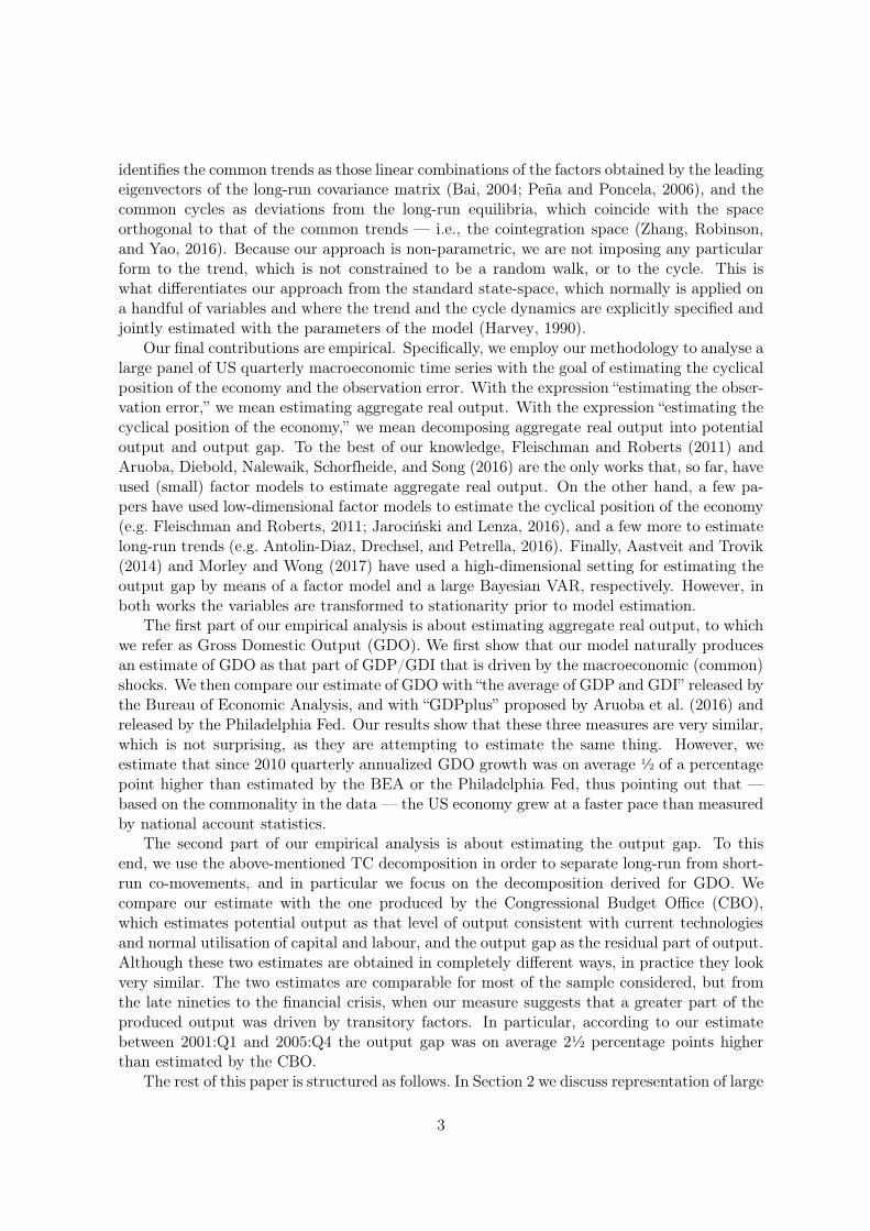


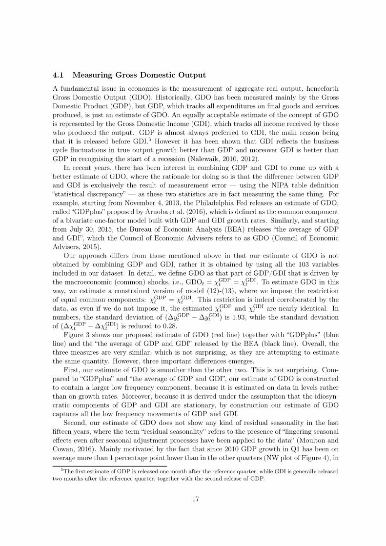
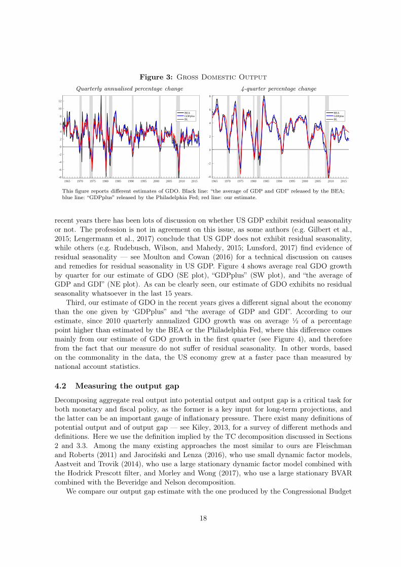


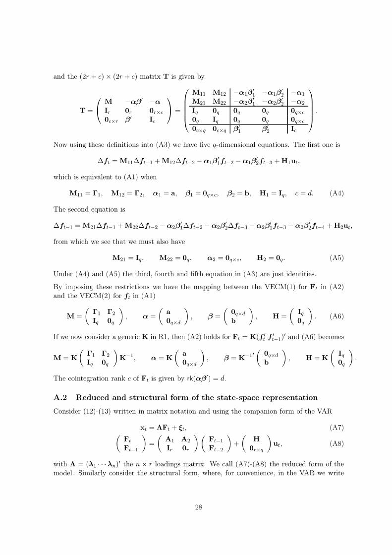


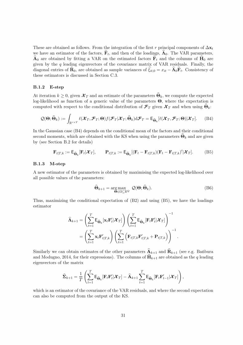


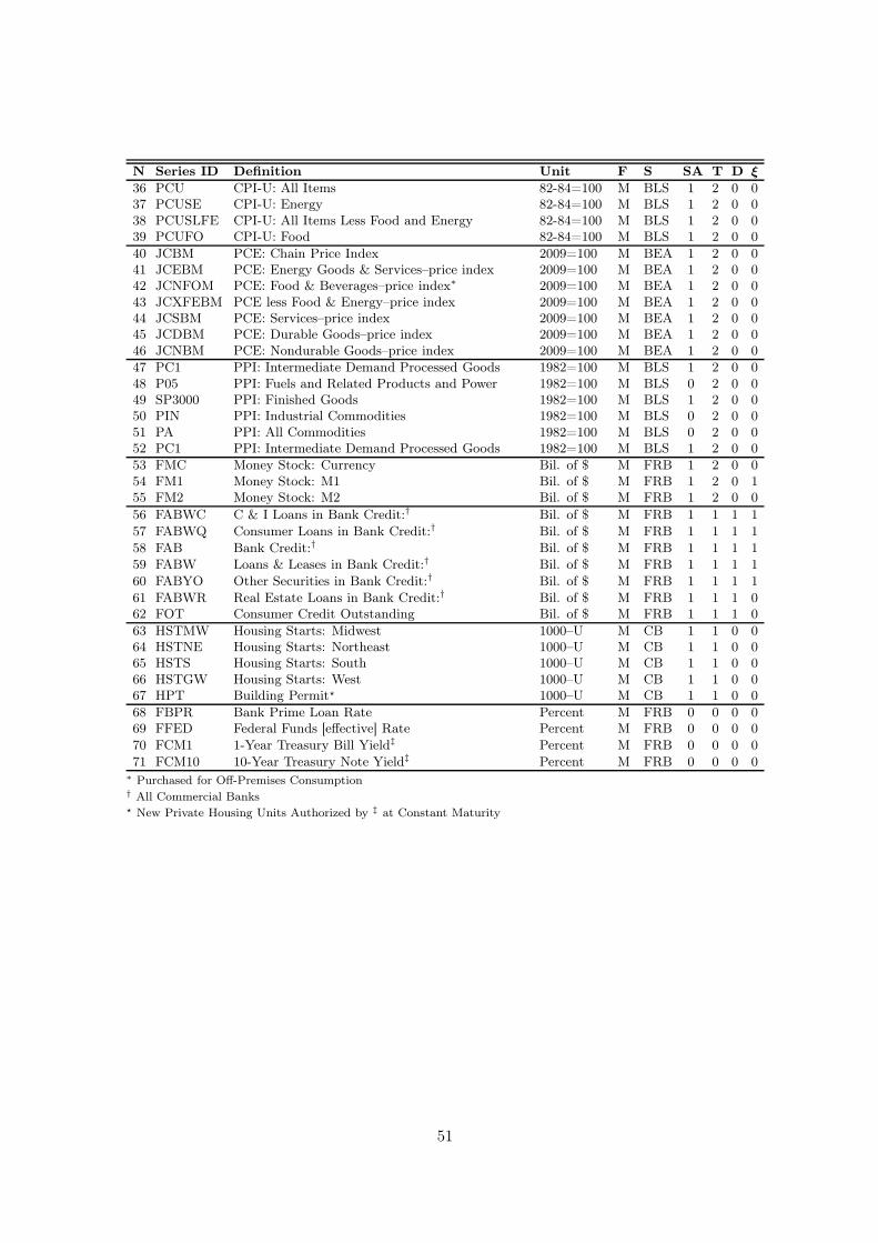


![Cemetery Records by Last Name - hshccatalog.org · Aaronson, Harry E. 1955 Saint George's Episcopal Church [Spesutia] Aaronson, Henrietta R. 1960 Baker Cemetery Aaronson, James K.](https://static.documents.pub/doc/80x56/5f039ec67e708231d409f368/cemetery-records-by-last-name-aaronson-harry-e-1955-saint-georges-episcopal.jpg)


