Faculty of Engineering Electrical Engineering Department Communication II Lab (EELE 4170) Lab#1 Sampling and Quantization Objectives: 1-To understand the theory and application of sampling and quantization. 2-To understand the effect of aliasing on the reconstruction process. Theory: 1-Sampling theorem A real signal whose spectrum is band limited to f (Hz) can be reconstructed exactly (without any error) from its samples taken uniformly at a rate fs > 2f (samples per second). In other words the minimum sampling frequency is fs = 2 f. To prove sampling theorem, assume an analog waveform x (t), as shown in figure 1(a), with a Fourier transform, X (f) which is zero outside the interval (− fm < f < fm), as shown in figure 3(b). The sampling of x (t) can be viewed as the product of x (t) with a periodic train of unit impulse function (t), shown in figure 3(c) and defined as = ( − ) ∞ =−∞ Where the sampling period and δ (t) is is the unit impulse. Let us choose =1/2f s , so that the Nyquist criterion is just satisfied. The sifting property (the product of a function with an impulse () is equal to the value of that function at the instant at which the impulse is located) of the impulse function states that − = (− ) Using the frequency convolution property of the Fourier transform we can transform the time-domain product () to the frequency-domain convolution ∗ () , = 1 ( − ) ∞ =−∞
Transcript
Faculty of Engineering
Electrical Engineering Department
Communication II Lab (EELE 4170)
Lab#1 Sampling and Quantization
Objectives:
1-To understand the theory and application of sampling and quantization.
2-To understand the effect of aliasing on the reconstruction process.
Theory:
1-Sampling theorem
A real signal whose spectrum is band limited to f (Hz) can be reconstructed exactly (without any error) from its samples taken uniformly at a rate fs > 2f (samples per second). In other words the minimum sampling frequency is fs = 2 f.
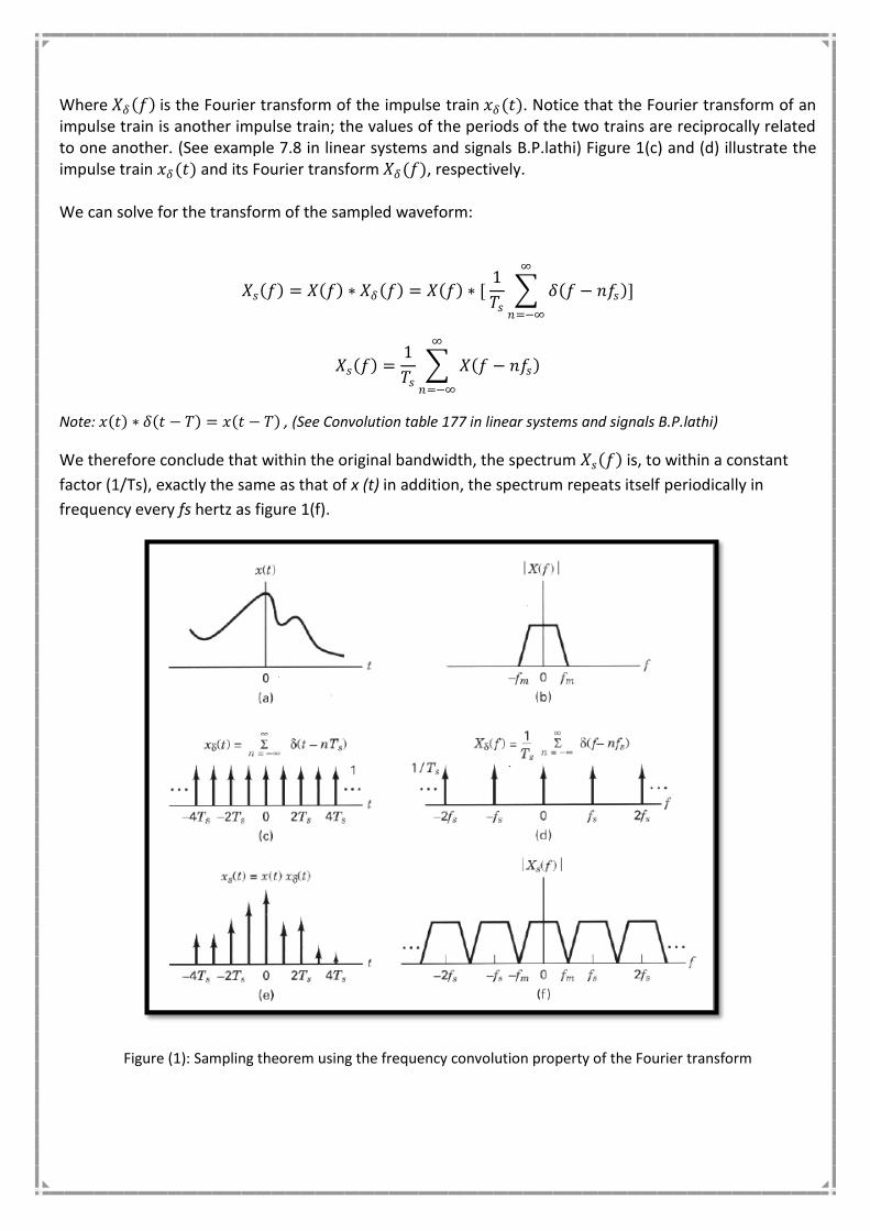
To prove sampling theorem, assume an analog waveform x (t), as shown in figure 1(a), with a Fourier
transform, X (f) which is zero outside the interval (− fm < f < fm), as shown in figure 3(b). The sampling of x (t) can be viewed as the product of x (t) with a periodic train of unit impulse function 𝑥𝛿 (t), shown in figure 3(c) and defined as
𝑥𝛿 𝑡 = 𝛿(𝑡 − 𝑛𝑇𝑠)
∞
𝑛=−∞
Where 𝑇𝑠the sampling period and δ (t) is is the unit impulse. Let us choose 𝑇𝑠=1/2fs, so that the Nyquist criterion is just satisfied. The sifting property (the product of a function with an impulse 𝛿(𝑡) is equal to the value of that function at the instant at which the impulse is located) of the impulse function states that
𝑥 𝑡 𝛿 𝑡 − 𝑡𝑜 = 𝑥 𝑡𝑜 𝛿(𝑡 − 𝑡𝑜) Using the frequency convolution property of the Fourier transform we can transform the time-domain product 𝑥 𝑡 𝑥𝛿(𝑡) to the frequency-domain convolution 𝑋 𝑓 ∗ 𝑋𝛿(𝑓) ,
𝑋𝛿 𝑓 =1
𝑇𝑠 𝛿(𝑓 − 𝑛𝑓𝑠)
∞
𝑛=−∞
Where 𝑋𝛿 𝑓 is the Fourier transform of the impulse train 𝑥𝛿(𝑡). Notice that the Fourier transform of an impulse train is another impulse train; the values of the periods of the two trains are reciprocally related to one another. (See example 7.8 in linear systems and signals B.P.lathi) Figure 1(c) and (d) illustrate the impulse train 𝑥𝛿(𝑡) and its Fourier transform 𝑋𝛿(𝑓), respectively. We can solve for the transform of the sampled waveform:
𝑋𝑠 𝑓 = 𝑋 𝑓 ∗ 𝑋𝛿 𝑓 = 𝑋 𝑓 ∗ [ 1
𝑇𝑠 𝛿 𝑓 − 𝑛𝑓𝑠
∞
𝑛=−∞
]
𝑋𝑠 𝑓 =1
𝑇𝑠 𝑋 𝑓 − 𝑛𝑓𝑠
∞
𝑛=−∞
Note: 𝑥 𝑡 ∗ 𝛿 𝑡 − 𝑇 = 𝑥 𝑡 − 𝑇 , (See Convolution table 177 in linear systems and signals B.P.lathi)
We therefore conclude that within the original bandwidth, the spectrum 𝑋𝑠 𝑓 is, to within a constant
factor (1/Ts), exactly the same as that of x (t) in addition, the spectrum repeats itself periodically in
frequency every fs hertz as figure 1(f).
Figure (1): Sampling theorem using the frequency convolution property of the Fourier transform
0 0.1 0.2 0.3 0.4 0.5 0.6 0.7 0.8 0.9 1-1
-0.8
-0.6
-0.4
-0.2
0
0.2
0.4
0.6
0.8
1
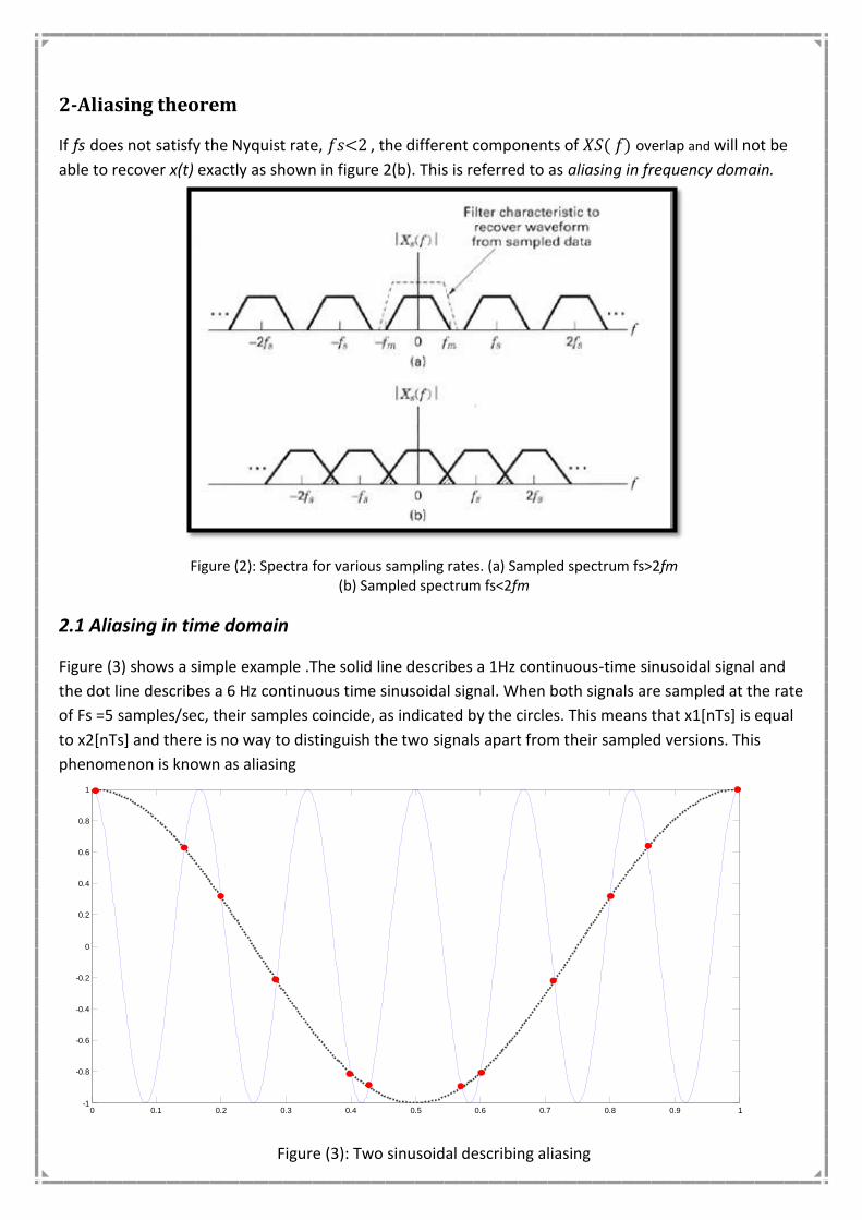
2-Aliasing theorem
If fs does not satisfy the Nyquist rate, 𝑓𝑠<2 , the different components of 𝑋𝑆( 𝑓) overlap and will not be
able to recover x(t) exactly as shown in figure 2(b). This is referred to as aliasing in frequency domain.
Figure (2): Spectra for various sampling rates. (a) Sampled spectrum fs>2fm (b) Sampled spectrum fs<2fm
2.1 Aliasing in time domain
Figure (3) shows a simple example .The solid line describes a 1Hz continuous-time sinusoidal signal and
the dot line describes a 6 Hz continuous time sinusoidal signal. When both signals are sampled at the rate
of Fs =5 samples/sec, their samples coincide, as indicated by the circles. This means that x1[nTs] is equal
to x2[nTs] and there is no way to distinguish the two signals apart from their sampled versions. This
Where 𝐹𝑎𝑙𝑖𝑎𝑠𝑒𝑑 𝑎𝑛𝑑 𝑓𝑎𝑙𝑖𝑎𝑠𝑒𝑑 are outside the fundamental frequency range:
−𝐹𝑠2
≤ 𝐹𝑏𝑎𝑠𝑒 ≤𝐹𝑠2
𝑎𝑛𝑑 −1
2≤ 𝑓𝑏𝑎𝑠𝑒 ≤
1
2
In order to avoid aliasing we must restrict the analog signal x (t) to the frequency range, F less than Fs/2.
Thus, every sampler must be preceded by an analog low-pass filter, known as an anti-aliasing filter; with a
cut-off frequency fc equals fs /2.
3- Quantization
The second stage in the A/D process is amplitude quantization, where the sampled discrete-time signal x(n), is quantized into a finite set of output levels . The quantized signal can take only one of L levels, which are designed to cover the dynamic range:
xmin ≤ x(n) ≤ xmax
The step size or resolution of the uniform quantizer is given as:
∆=𝑋𝑚𝑖𝑛 − 𝑋𝑚𝑎𝑥
𝐿 − 1
The step size can be either integer or fraction and is determined by the number of levels L. For binary coding, L is usually a power of 2, and practical values are 256 (=2 ^8) or greater. The difference between the actual analog value and quantized digital value is called quantization error.
Quantization error = 𝑒𝑞 𝑛 = 𝑥𝑞 𝑛 − 𝑥(𝑛)
−∆
2≤ 𝑒𝑟𝑟𝑜𝑟 ≤
∆
2
Practical parts:
Part1: Sampling and aliasing
The signal 𝑥 𝑡 = cos 2𝜋𝐹𝑡 can be sampled at rate 𝐹𝑠 =1
𝑇𝑠 to yield 𝑥[𝑛] = cos(2𝜋
𝐹
𝐹𝑠𝑛).
1. Let F = 800 Hz and Fs =40 kHz .compute and plot x[n].
2. Let F1=200 Hz, F2=800Hz and Fs =40kHz.compute and plot x[n].
3. Let F1=39800 Hz, F2=39200Hz and Fs =40kHz.compute and plot x[n].
Fs=40000;
F=800;
n=0:100;
xn=cos(2*pi*(F/Fs)*n);
stem(xn)
figure(1)
Fs=40000;
n=0:100;
Fo=[200,800];
for i=1:2;
subplot(2,1,i)
xn=cos(2*pi*(Fo(i)/Fs)*n);
stem(xn)
end
figure(2)
Fs=40000;
n=0:100;
Fo=[39800,39200];
for i=1:2;
subplot(2,1,i)
xn=cos(2*pi*(Fo(i)/Fs)*n);
stem(xn)
end
0 0.1 0.2 0.3 0.4 0.5 0.6 0.7 0.8 0.9 1-1
-0.5
0
0.5
1
0 0.1 0.2 0.3 0.4 0.5 0.6 0.7 0.8 0.9 10
0.5
1
1.5
2
2.5
3
0 0.1 0.2 0.3 0.4 0.5 0.6 0.7 0.8 0.9 10
0.5
1
1.5
2
2.5
3
0 0.1 0.2 0.3 0.4 0.5 0.6 0.7 0.8 0.9 1-1
-0.5
0
0.5
1
Part2: Quantization
1. Write a Matlab function Y = uquant(X, L) which will uniformly quantize an input array X (either a vector or a matrix) to L discrete levels.
2. Use this function to quantize an analog sinusoidal signal x(t)=sin(2*pi*t) with L=4 and 32 levels.


![[4170]-281unipune.ac.in/university_files/pdf/old_papers/April2012/...importance of Timing and Scheduling of Operations. [4170]-281 1 P.T.O. Seat No. [4170]-281/2 Q.4) Explain the situations](https://static.documents.pub/doc/80x56/5af4a3db7f8b9a92718dcf84/4170-of-timing-and-scheduling-of-operations-4170-281-1-pto-seat-no-4170-2812.jpg)


