51

FEEG6017 lecture:
Bayes' theorem and
Bayesian estimation
Dr Brendan Neville
Null hypothesis significance
testing: what are we doing?
• When we report on a p-value, we're
describing the probability of observing our
data (or more extreme data) given the
assumption that the null hypothesis is true.
• The convention is that if this probability is
low enough, we decide to reject the null
hypothesis and tentatively adopt the
alternative hypothesis.

Null hypothesis significance
testing: what are we doing?
• The difficulty in interpreting p-values is that
it's tempting to see them as somehow
describing the probability of the model being
correct.
• (A natural confusion: the appropriateness of
our model is what we really care about.)
• But p-values don't do this, they describe the
probability of the data given a very boring
model, the null hypothesis.
• P(Data|Null)
The null hypothesis: over-rated?
• In fact we're often not much interested in the
null hypothesis: in almost all realistic cases
it's not true.
• We could demonstrate that by collecting
more data, and/or measuring more precisely.
• The null hypothesis has had a starring role in
the history of statistics simply because it is
mathematically convenient.

Integrating new evidence
• It's a familiar scientific activity to report on
the p-value of some analysis and, if it's low
enough, to publish the findings.
• But how should we integrate new evidence
over time though?
Integrating new evidence
• Suppose many scientists investigate some
phenomenon.
• Most find that an effect exists, e.g., a
positive relationship between basketball skill
and height.
• Some analyses have very low p-values,
others are marginal, still others are non-
significant.

Integrating new evidence
• How should we rationally combine the
conclusions of these studies?
• In fact in the real world of publication, there's
reason to be concerned that we don't do this
at all rationally...
• Some fields tend to use significance levels of
p=0.01 or p=0.05 as a threshold for
publication.

Dangers of publication bias
• There's also an interest in publishing "new"
and "exciting" results.
• John Ioannidis's paper "Why most published
research findings are false" points out that
NHST combined with publication bias is a
recipe for disaster.
• Half-life of knowledge.
• Nevertheless: most of us have a pragmatic
sense of evidence somehow accumulating
for (or against) a theory over time.

Frequentist thinking
• There are several schools of thought on
probability.
• One is the "frequentist" view, which says
probabilities can only refer to the objective
long-run frequency of an event occurring in a
well-defined sample space.
• Particular events either happen or they don't.

Probability and belief
• Frequentists disapprove of using
probabilities to refer to subjective belief.
• For example: "I am 90% sure that he is the
one who stole the coffee money." Are we
happy with this kind of talk?
• Bayesian thinking: if we allow probabilities to
refer to subjective belief, this turns out to
help with the integration of new information.
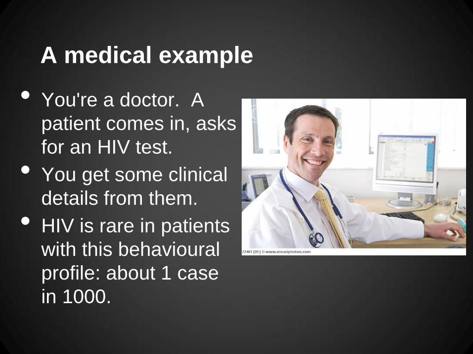
A medical example
• You're a doctor. A
patient comes in, asks
for an HIV test.
• You get some clinical
details from them.
• HIV is rare in patients
with this behavioural
profile: about 1 case
in 1000.
A medical example
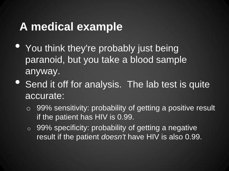
• You think they're probably just being
paranoid, but you take a blood sample
anyway.
• Send it off for analysis. The lab test is quite
accurate:
o 99% sensitivity: probability of getting a positive result
if the patient has HIV is 0.99.
o 99% specificity: probability of getting a negative
result if the patient doesn't have HIV is also 0.99.

A medical example
• To your surprise, the test comes back
positive.
• The patient is understandably dismayed, and
asks "Could it be a mistake?". What is the
probability that the patient has HIV?
• If you haven't seen this kind of problem
before, take a minute to think about your
answer.

A medical example
• The real answer is about 0.0902, or 9.02%.
• Only around 15% of doctors get this right.
• Many respondents focus on the 99%
sensitivity of the test, and believe that the
patient is 99% likely to have HIV given the
positive result.
• They're neglecting the background or base
rate of HIV prevalence.

Test example with frequencies
• Doctors (and others) do a better job on the
problem if it is framed differently.
• Consider a population of 100,000 people
who each decide to have an HIV test.
• HIV is rare in this population: 100 people
have it, and 99,900 people do not.
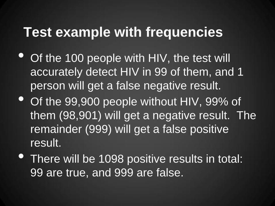
Test example with frequencies
• Of the 100 people with HIV, the test will
accurately detect HIV in 99 of them, and 1
person will get a false negative result.
• Of the 99,900 people without HIV, 99% of
them (98,901) will get a negative result. The
remainder (999) will get a false positive
result.
• There will be 1098 positive results in total:
99 are true, and 999 are false.

Test example with frequencies
• The probability of actually having HIV after
getting a positive test result is therefore
99 / 1098 = 0.0902.
• (Do you agree that this version makes the
problem easier?)
• The logic expressed here is Bayes' theorem.
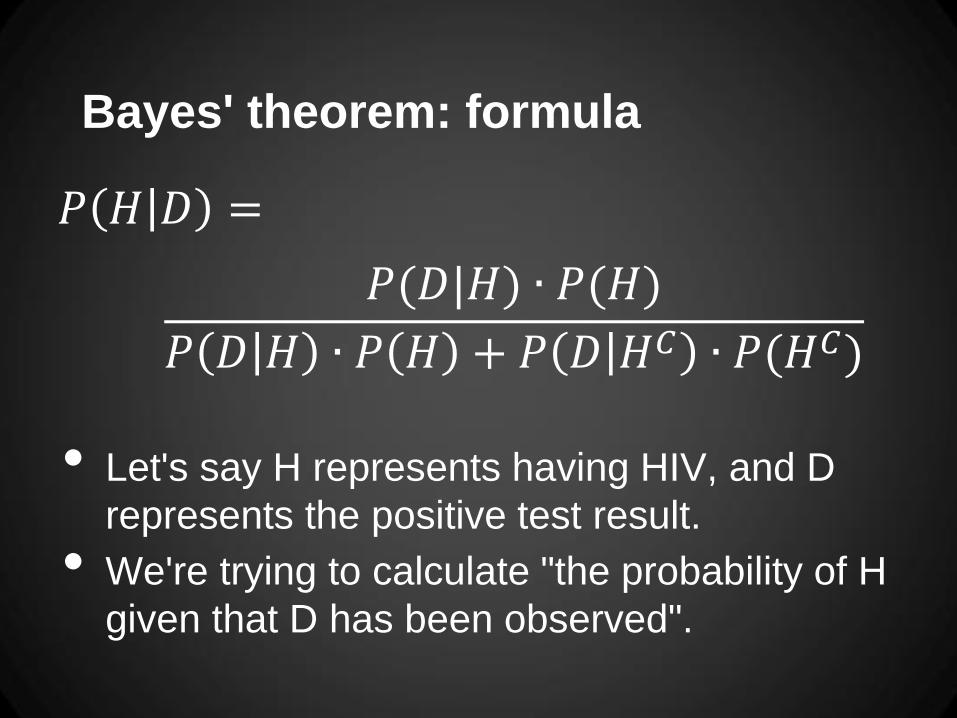
Bayes' theorem: formula
𝑃 𝐻 𝐷 =
𝑃(𝐷|𝐻) ∙ 𝑃(𝐻)
𝑃 𝐷 𝐻 ∙ 𝑃 𝐻 + 𝑃 𝐷 𝐻𝐶 ∙ 𝑃(𝐻𝐶)
• Let's say H represents having HIV, and D
represents the positive test result.
• We're trying to calculate "the probability of H
given that D has been observed".
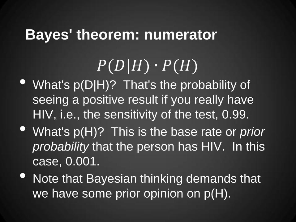
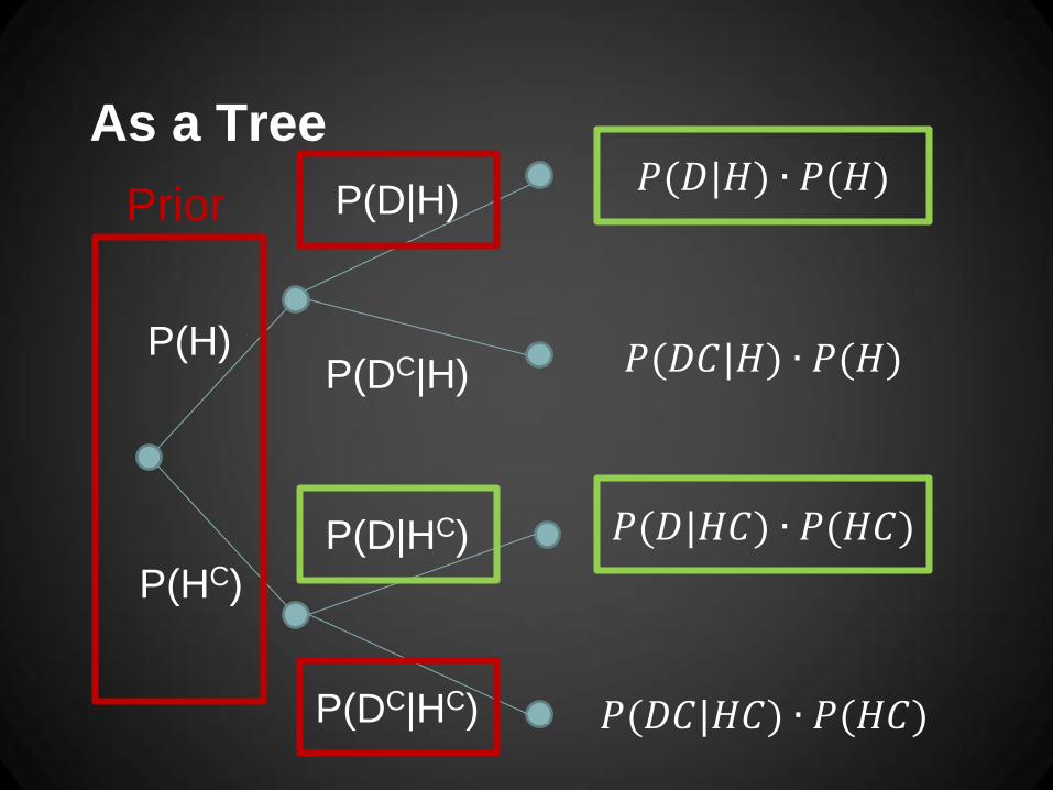
Bayes' theorem: numerator
𝑃(𝐷|𝐻) ∙ 𝑃(𝐻) • What's p(D|H)? That's the probability of
seeing a positive result if you really have
HIV, i.e., the sensitivity of the test, 0.99.
• What's p(H)? This is the base rate or prior
probability that the person has HIV. In this
case, 0.001.
• Note that Bayesian thinking demands that
we have some prior opinion on p(H).

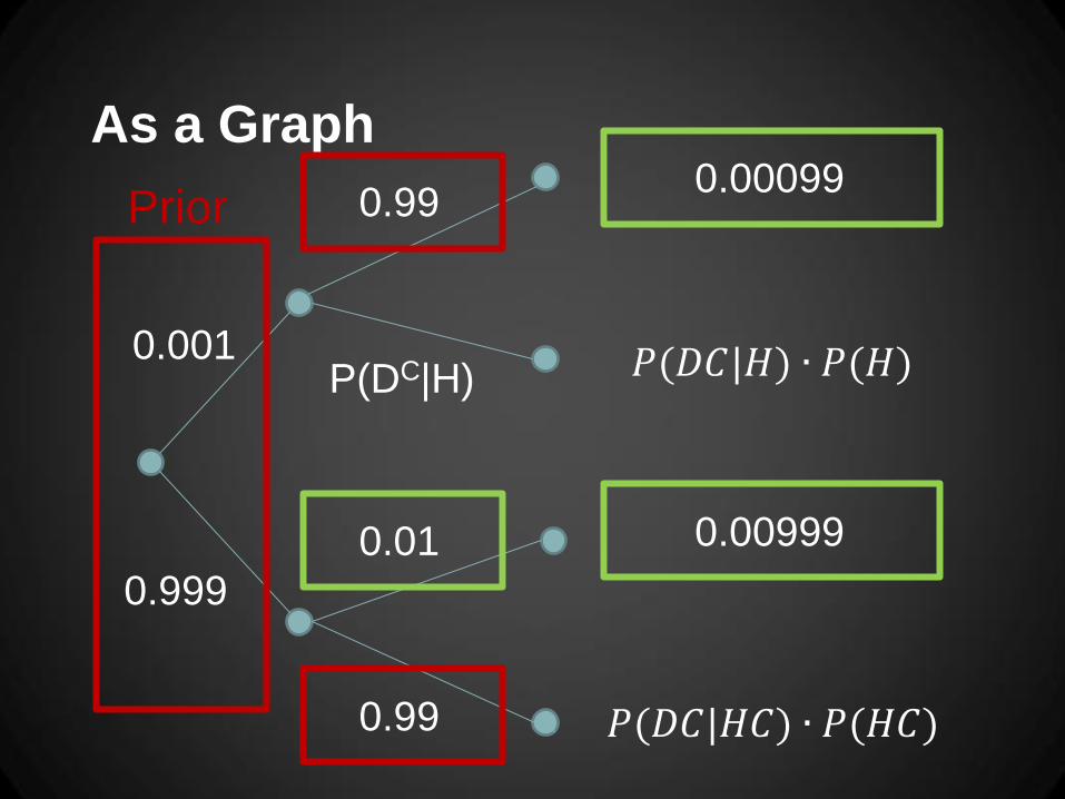
Bayes' theorem: numerator
• So the numerator is:
𝑃(𝐷|𝐻) ∙ 𝑃(𝐻)
0.99 x 0.001 = 0.00099
• This is the probability of any one person both
having HIV and also returning a positive
result on the test.

Bayes' theorem: denominator
𝑃 𝐷 𝐻 ∙ 𝑃 𝐻 + 𝑃 𝐷 𝐻𝐶 ∙ 𝑃(𝐻𝐶)
• The first component of the denominator
simply repeats the numerator.
• This is "how often does someone have HIV
and then get a positive test result“.
• The second component looks at the other
way you can get a positive test result, i.e.,
via a false positive.

Bayes' theorem: denominator
• We need to know P(D|HC), i.e., the
probability of seeing a positive test result if
you don't have HIV. That's 0.01, the
complement of the specificity.
• We also want to know P(HC), the prior
probability of not having HIV. That's 0.999.
• Multiply them to get the overall rate of false
positives: 0.01 x 0.999 = 0.00999.

Bayes' theorem: denominator
• We add these two components to find out
how often positive test results will be seen
for any reason:
𝑃 𝐷 𝐻 ∙ 𝑃 𝐻 + 𝑃 𝐷 𝐻𝐶 ∙ 𝑃(𝐻𝐶)
0.00099 + 0.00999 = 0.01098
• So about 1% of the time we'll see positive
test results.
• How often will those be true positives? In
other words, what's p(H|D)?

Bayes' theorem:
putting it all together
• The probability of seeing a true positive
(0.00099)...
... divided by the overall probability of seeing
a positive test result of either sort (0.01098)
... gives the probability of actually having HIV
given the observation of a positive test result
(0.09016).
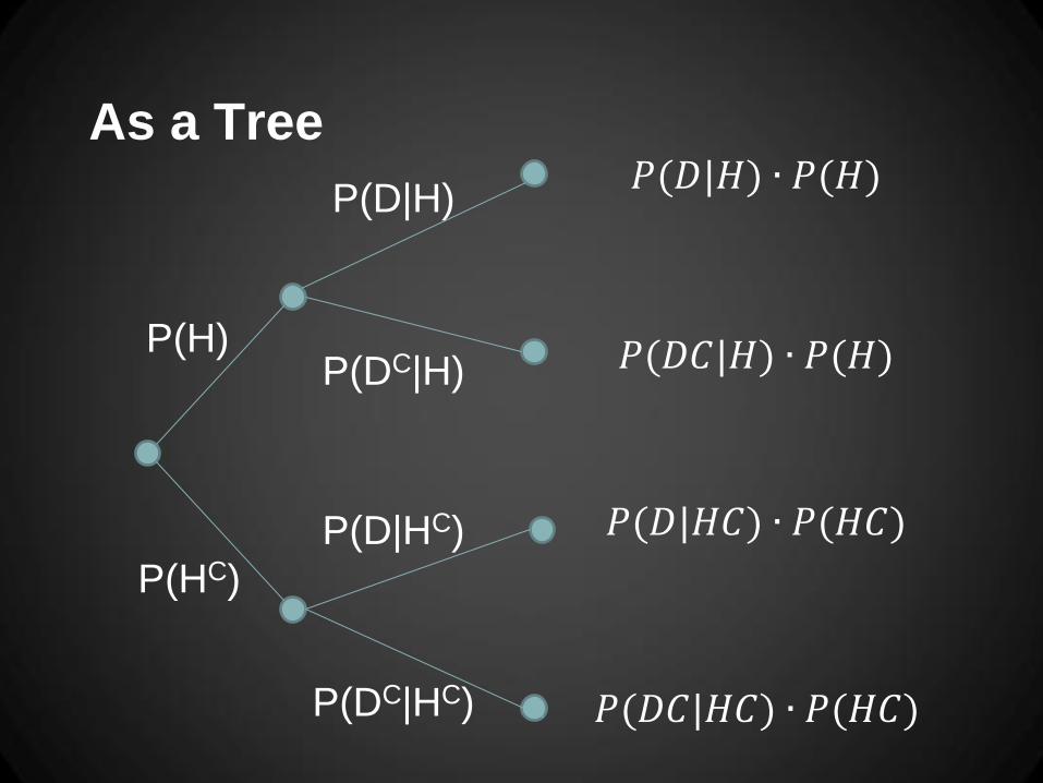
As a Tree
P(H)
P(HC)
P(D|H)
P(DC|H)
P(D|HC)
P(DC|HC)
𝑃(𝐷|𝐻) ∙ 𝑃(𝐻)
𝑃(𝐷𝐶|𝐻) ∙ 𝑃(𝐻)
𝑃(𝐷|𝐻𝐶) ∙ 𝑃(𝐻𝐶)
𝑃(𝐷𝐶|𝐻𝐶) ∙ 𝑃(𝐻𝐶)

As a Tree
P(H)
P(HC)
P(D|H)
P(DC|H)
P(D|HC)
P(DC|HC)
𝑃(𝐷|𝐻) ∙ 𝑃(𝐻)
𝑃(𝐷𝐶|𝐻) ∙ 𝑃(𝐻)
𝑃 𝐷 𝐻𝐶 ∙ 𝑃(𝐻𝐶)
𝑃(𝐷𝐶|𝐻𝐶) ∙ 𝑃(𝐻𝐶)
As a Tree
P(H)
P(HC)
P(D|H)
P(DC|H)
P(D|HC)
P(DC|HC)
𝑃(𝐷|𝐻) ∙ 𝑃(𝐻)
𝑃(𝐷𝐶|𝐻) ∙ 𝑃(𝐻)
𝑃(𝐷|𝐻𝐶) ∙ 𝑃(𝐻𝐶)
𝑃(𝐷𝐶|𝐻𝐶) ∙ 𝑃(𝐻𝐶)
Prior

As a Graph
0.001
0.999
0.99
P(DC|H)
P(D|HC)
0.99
𝑃(𝐷|𝐻) ∙ 𝑃(𝐻)
𝑃(𝐷𝐶|𝐻) ∙ 𝑃(𝐻)
𝑃(𝐷|𝐻𝐶) ∙ 𝑃(𝐻𝐶)
𝑃(𝐷𝐶|𝐻𝐶) ∙ 𝑃(𝐻𝐶)
Prior

As a Graph
0.001
0.999
0.99
P(DC|H)
0.01
0.99
𝑃(𝐷|𝐻) ∙ 𝑃(𝐻)
𝑃(𝐷𝐶|𝐻) ∙ 𝑃(𝐻)
𝑃(𝐷|𝐻𝐶) ∙ 𝑃(𝐻𝐶)
𝑃(𝐷𝐶|𝐻𝐶) ∙ 𝑃(𝐻𝐶)
Prior
As a Graph
0.001
0.999
0.99
P(DC|H)
0.01
0.99
0.00099
𝑃(𝐷𝐶|𝐻) ∙ 𝑃(𝐻)
0.00999
𝑃(𝐷𝐶|𝐻𝐶) ∙ 𝑃(𝐻𝐶)
Prior

Bayes' theorem: formula
𝑃 𝐻 𝐷 =𝑃(𝐷|𝐻) ∙ 𝑃(𝐻)
𝑃 𝐷 𝐻 ∙ 𝑃 𝐻 + 𝑃 𝐷 𝐻𝐶 ∙ 𝑃(𝐻𝐶)
𝑃 𝐻 𝐷 =0.99 x 0.001
(0.99 x 0.001)+(0.01 x 0.999)
𝑃(𝐻|𝐷) =0.00099
0.01098= 0.09016
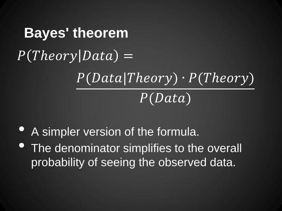
Bayes' theorem
𝑃 𝑇ℎ𝑒𝑜𝑟𝑦 𝐷𝑎𝑡𝑎 =
𝑃(𝐷𝑎𝑡𝑎|𝑇ℎ𝑒𝑜𝑟𝑦) ∙ 𝑃(𝑇ℎ𝑒𝑜𝑟𝑦)
𝑃(𝐷𝑎𝑡𝑎)
• A simpler version of the formula.
• The denominator simplifies to the overall
probability of seeing the observed data.

Rethinking the test example
• Let's view the doctor as a scientist who is
collecting data. He starts with the estimated
prior probability for a patient to have HIV of
0.001.
• He makes a measurement (i.e., the HIV
test).
• The measurement forces a change in the
estimated probability that the patient has
HIV.
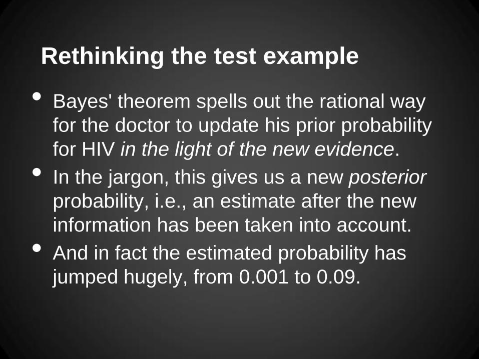
Rethinking the test example
• Bayes' theorem spells out the rational way
for the doctor to update his prior probability
for HIV in the light of the new evidence.
• In the jargon, this gives us a new posterior
probability, i.e., an estimate after the new
information has been taken into account.
• And in fact the estimated probability has
jumped hugely, from 0.001 to 0.09.
Another example: finding the mole
• This is a story in the style of John le Carré in
order to make clear the link between Bayes'
theorem and the revision or updating of
scientific theories.
• So: you're the head of MI6. You're pretty
sure there's a "mole" in your organization.
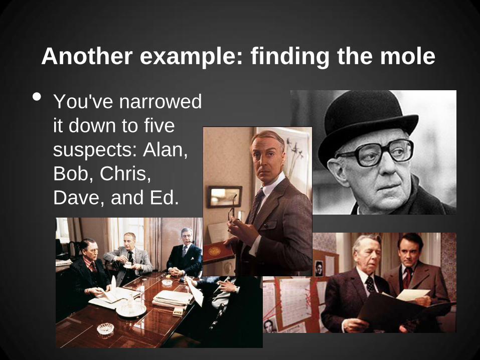
Another example: finding the mole
• You've narrowed
it down to five
suspects: Alan,
Bob, Chris,
Dave, and Ed.

Finding the mole
• You have all five arrested and begin to
interrogate them.
• You know from previous experience with
interrogations that there are five behaviours
to be expected in any given session: normal
behaviour, nervousness, anger at the
accusation, making a mistake in one's story,
and a desperate exhausted confession.
Finding the mole
• However, none of these five behaviours will
completely settle the question.
• Both moles and loyal operatives will exhibit
any of these, even confession.
• However, you know from experience that
moles and loyal operatives will exhibit the
five behaviours at different rates.

Behaviours of loyal operatives

Behaviours of moles

Prior probabilities
• Perhaps you have no idea who the mole is,
but are convinced that it must be one of the
suspects.
• The probability-of-being-the-mole is 0.2 for
each person in this case. This is called a
uniform prior.
Iterative Bayesian reasoning
• We begin the interrogation sessions.
• After each session, we update our prior
probability estimate of each person being the
mole using Bayes' theorem.
• We then return to the questioning, but
today's posterior becomes tomorrow's prior.

Iterative Bayesian reasoning
Session 1
Alan (0.2) Normal 0.164
Bob (0.2) Normal 0.164
Chris (0.2) Confess 0.333
Dave (0.2) Normal 0.164
Ed (0.2) Normal 0.164
Session 2
Alan (0.164) Normal 0.134
Bob (0.164) Mistake 0.164
Chris (0.333) Nervous 0.429
Dave (0.164) Normal 0.134
Ed (0.164) Confess 0.282
Uniform Priors
P(M|L)=P(M|LC)
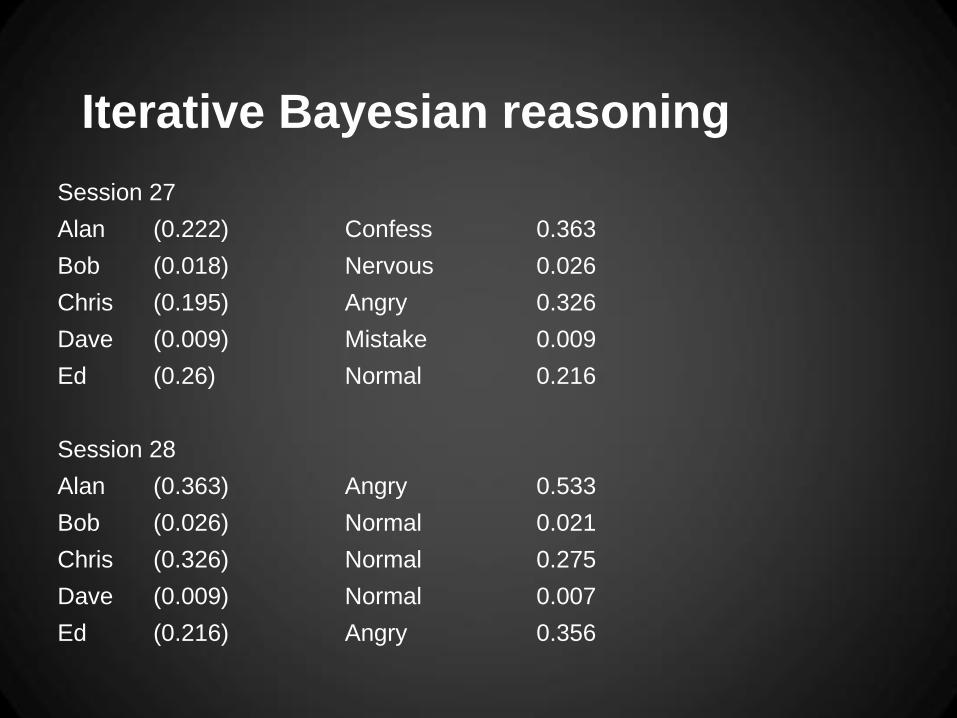
Iterative Bayesian reasoning
Session 27
Alan (0.222) Confess 0.363
Bob (0.018) Nervous 0.026
Chris (0.195) Angry 0.326
Dave (0.009) Mistake 0.009
Ed (0.26) Normal 0.216
Session 28
Alan (0.363) Angry 0.533
Bob (0.026) Normal 0.021
Chris (0.326) Normal 0.275
Dave (0.009) Normal 0.007
Ed (0.216) Angry 0.356

Iterative Bayesian reasoning
Session 150
Alan (0.0) Normal 0.0
Bob (0.0) Normal 0.0
Chris (0.999) Confess 1.0
Dave (0.001) Confess 0.001
Ed (1.0) Normal 1.0
• The truth is there are two moles: Chris and
Ed. After enough sessions, our probability
estimates reflect this.

Prior probabilities
• But perhaps you are not so agnostic:
o Alan is your oldest friend; you can't believe it could
be him. You assign him a prior of 0.001.
o Bob seems unlikely, but you never know: 0.1.
o Chris, well, you never liked his face: 0.5.
o Dave has been taking a lot of mysterious holidays to
Moscow: 0.75.
o Ed: surely not? 0.05.
• The probabilities don't add to 1.0 as there
just might be more than one of them!
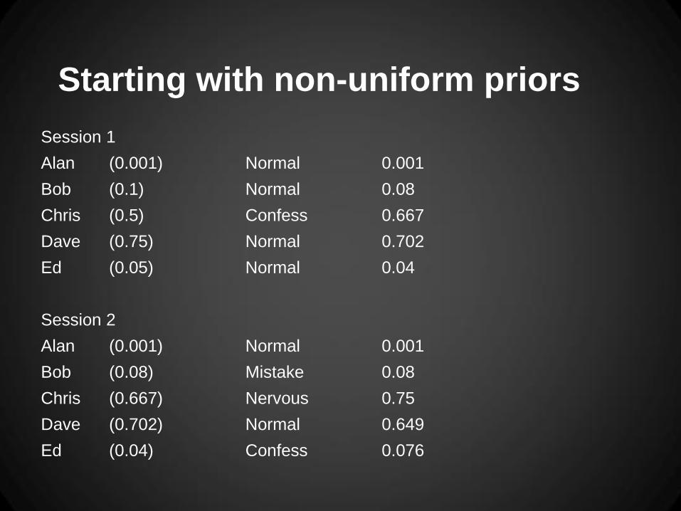
Starting with non-uniform priors
Session 1
Alan (0.001) Normal 0.001
Bob (0.1) Normal 0.08
Chris (0.5) Confess 0.667
Dave (0.75) Normal 0.702
Ed (0.05) Normal 0.04
Session 2
Alan (0.001) Normal 0.001
Bob (0.08) Mistake 0.08
Chris (0.667) Nervous 0.75
Dave (0.702) Normal 0.649
Ed (0.04) Confess 0.076

Starting with non-uniform priors
Session 150
Alan (0.0) Normal 0.0
Bob (0.0) Normal 0.0
Chris (1.0) Confess 1.0
Dave (0.009) Confess 0.017
Ed (1.0) Normal 1.0
• We get to the same estimates eventually.
We started out badly wrong about Dave and
Ed, but with enough data, our priors don't
matter.
Bayesian statistics?
• Explicitly Bayesian statistical procedures
exist, in which new data is used to update
priors.
o These were not really practical before the era of
computational statistical tools.
o Often used in machine learning or artificial
intelligence: e.g., how should a robot use sensory
input to update its estimate of where the target is?

Bayesian statistics?
• Bayes-inspired procedures exist, e.g., the
Bayesian Information Criterion; similar to the
AIC measure.
• Bayes as a mindset.
o Comparing models and searching for the current
best one is a better statistical practice than repeated
use of NHST.
o Preferred model will change as more data comes in.

Additional material
• Great online intro to Bayesian thinking.
• Python program used to produce the "find
the mole" example.


![Bayesian InferenceStatisticat].pdf1. Bayes’ Theorem Bayes’ theorem shows the relation between two conditional probabilities that are the reverse of each other. This theorem is](https://static.documents.pub/doc/80x56/5f8dd532af152601480d83ba/bayesian-inference-statisticatpdf-1-bayesa-theorem-bayesa-theorem-shows-the.jpg)


