SEC “ 5 ”SIMPLE LINEAR REGRESSION

BAYES' THEOREM

Simple Linear Regression

• Linear regression models are used to describe or predict the relationship between two variables

“ 𝑥 and 𝑦 “. The simple linear regression model is represented by:

𝑦 = 𝛽0 + 𝛽1𝑥 + 𝑒

𝜷𝟎

𝜷𝟏

𝑦 : The factor that is being predicted (the factor that the equation

solves for) is called the dependent variable.

𝑥 : The factors that are used to predict the value of the

dependent variable are called the independent variables.

𝑒 : Is the error of the estimate. The error term is used to account

for the variability in 𝑦 that cannot be explained by the linear

relationship between 𝑥 and 𝑦.

𝛽0 : Is the y-intercept of the regression line.

𝛽1 : Is the slope.

The Estimated Linear Regression Equation

• In practice, the parameter of the population values generally are not known so they must

be estimated by using data from a sample of the population. The population parameters

are estimated by using sample statistics. The sample statistics are represented by 𝑏0 and

𝑏1. When the sample statistics are substituted for the population parameters, the estimated

regression equation is formed as follow:

𝐸 𝑦 = ො𝑦 = 𝑏0 + 𝑏1𝑥, 𝑤ℎ𝑒𝑟𝑒

𝑏0 = 𝐸 𝛽0 = 𝑦 − 𝑏1𝑥,

and

𝑏1 = 𝐸 𝛽1 = 𝑟𝑠𝑦

𝑠𝑥

• the error in the predicted value of 𝒚 at a

certain value of 𝒙:

Error = ෝ𝒚 − 𝒚• The coefficient of determination 𝒓𝟐:

how well does the regression equation fit the

data. This means that % of the variation in 𝒚can be described by 𝒙.

Sheet (3)

12. Last year, five randomly selected students took a math aptitude test before they

began their statistics course. The Statistics Department has three questions.

Student 𝒙𝒊 𝒚𝒊

1 95 85

2 85 95

3 80 70

4 70 65

5 60 70

• Draw the scatter plot representing the data

• What linear regression equation best predicts statistics performance, based on math

aptitude scores?

❑ 𝑛 = 5

❑ 𝑋 =σ𝑖=15 𝑥𝑖

𝑛=

95+⋯+60

5= 78

❑ 𝑠𝑥 =σ𝑖=15 𝑥−𝑥 2

𝑛−1=

95−78 2+⋯+ 95−78 2

4=13.5093

❑ 𝑦 =σ𝑖=15 𝑦𝑖

𝑛=

85+⋯+70

5= 77

❑ 𝑠𝑦 =σ𝑖=15 𝑦−𝑦 2

𝑛−1=

85−77 2+⋯+ 70−77 2

4=12.5499

❑ ො𝑦 = 𝑏0 + 𝑏1𝑥

➢ 𝑏1 = 𝑟𝑠𝑦

𝑠𝑥

= 0.693112.5499

13.5093

= 0.644

➢ 𝑏0 = 𝑦 − 𝑏1𝑥 = 77 − 0.644 ∗ 78

= 26.768

ො𝑦 = 26.768 + 0.644 𝑥

𝑥𝒛𝒙 =

𝒙 − 𝟕𝟖

𝟏𝟑. 𝟓𝟎𝟗𝟑

𝒚𝒛𝒚 =

𝒚 − 𝟕𝟕

𝟏𝟐. 𝟓𝟒𝟗𝟗

𝒛𝒙𝒛𝒚

95 1.2584 85 0.6375 0.8022

85 0.5182 95 1.4343 0.7433

80 0.1480 70 −0.5578 −0.0826

70 −0.5922 65 −0.9562 0.5663

60 −1.3324 70 −0.5578 0.7432

Total = 2.7724

𝑟 =σ𝑧𝑥𝑧𝑦𝑛 − 1

=2.7724

4= 0.6931

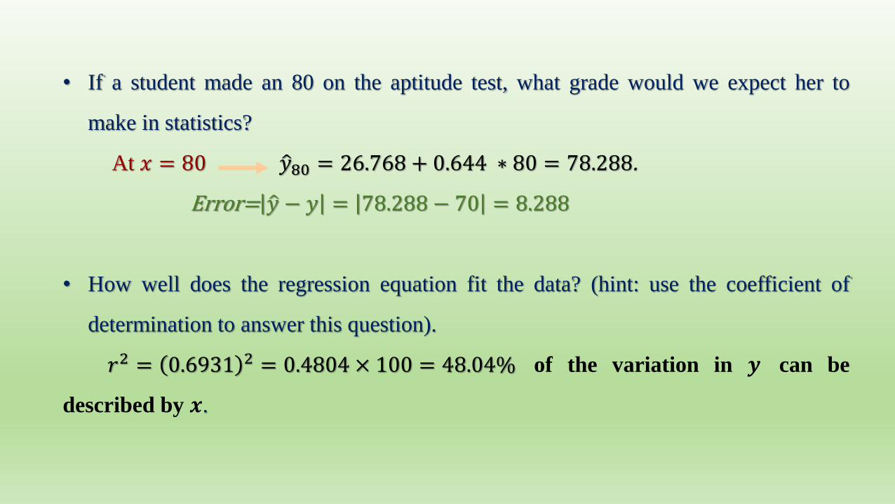
• If a student made an 80 on the aptitude test, what grade would we expect her to

make in statistics?

At 𝑥 = 80 ො𝑦80 = 26.768 + 0.644 ∗ 80 = 78.288.

Error= ො𝑦 − 𝑦 = 78.288 − 70 = 8.288

• How well does the regression equation fit the data? (hint: use the coefficient of

determination to answer this question).

𝑟2 = 0.6931 2 = 0.4804 × 100 = 48.04% of the variation in 𝒚 can be

described by 𝒙.

Bayes’ Rule

• Bayes' theorem, is a mathematical formula for determining conditional probability. Conditional

probability is the likelihood of an outcome occurring, based on a previous outcome occurring.

Bayes' theorem provides a way to revise existing predictions or theories (update probabilities)

given new or additional evidence

𝑨𝟏

𝑨𝟏

𝑨𝒌

…

𝑷 𝑨𝟐

𝟏

𝑩𝑷(𝑩|𝑨𝟏)

𝑷(𝑩|𝑨𝟐)

𝑷(𝑩|𝑨𝑲)

𝑩

𝑩

𝟐∩

𝑷(𝑨𝟏∩ 𝑩) = 𝑷(𝑩|𝑨𝟏)𝑷(𝑨𝟏)

𝑷(𝑨𝟐∩ 𝑩) = 𝑷(𝑩|𝑨𝟐)𝑷(𝑨𝟐)

𝑷(𝑨𝒌∩ 𝑩) = 𝑷(𝑩|𝑨𝒌)𝑷(𝑨𝒌)

……

𝑷 𝑩

➢ 𝑷 𝑩 = 𝑷(𝑨𝟏∩ 𝑩) + 𝑷(𝑨𝟐∩ 𝑩) +⋯+ 𝑷(𝑨𝒌∩ 𝑩)

= 𝑷(𝑩|𝑨𝟏)𝑷(𝑨𝟏) + 𝑷(𝑩|𝑨𝟐)𝑷(𝑨𝟐) + ⋯+ 𝑷(𝑩|𝑨𝒌)𝑷(𝑨𝒌)

= σ𝒋=𝟏𝒌 𝑷(𝑩|𝑨𝒋)𝑷(𝑨𝒋) “ Total Probability ” .

➢ 𝑷(𝑨𝒊 𝑩 =𝑷(𝑨𝒊∩𝑩)

𝑷 𝑩=

𝑷(𝑩|𝑨𝒊)𝑷(𝑨𝒊)

σ𝒋=𝟏𝒌 𝑷(𝑩|𝑨𝒋)𝑷(𝑨𝒋)

, 𝒊 = 𝟏, 𝟐, … , 𝒌

Sheet (3) [Revision on Probability]

4. All tractors made by a company are produced on one of three assembly lines, named Red,

White, and Blue. The chances that a tractor will not start when it rolls off of a line are 6%,

11%, and 8% for lines Red, White, and Blue, respectively. 48% of the company’s tractors

are made on the Red line and 31% are made on the Blue line.

(a) What fraction of the company’s tractors do not start when they roll off of an assembly

line?

𝑹

𝑩

𝑾

Let:

Red Line: R, Blue Line: B, White Line: W

Not Start “ Defective ”: D

𝑃 𝐷= 𝑃 𝑅 ∩ 𝐷 + 𝑃 𝐵 ∩ 𝐷 + 𝑃 𝑊 ∩ 𝐷= 0.0288 + 0.0248 + 0.0231= 0.0767 × 100= 7.67 ≈ 8%

𝑫

𝑫

𝑫

𝑷 𝑩 = 𝟎. 𝟑𝟏

𝑷 𝑫|𝑹 = 𝟎. 𝟎𝟔

𝑷 𝑫|𝑩 = 𝟎. 𝟎𝟖

𝑷 𝑫|𝑾 = 𝟎. 𝟏𝟏

∩

𝑷(𝑹 ∩ 𝑫) = 𝑷(𝑫|𝑹)𝑷(𝑹)= 𝟎. 𝟎𝟔 × 𝟎. 𝟒𝟖= 𝟎. 𝟎𝟐𝟖𝟖

𝑷(𝑩 ∩ 𝑫) = 𝑷(𝑫|𝑩)𝑷(𝑩)= 𝟎. 𝟎𝟖 × 𝟎. 𝟑𝟏= 𝟎. 𝟎𝟐𝟒𝟖

𝑷(𝑾∩𝑫) = 𝑷(𝑫|𝑾)𝑷(𝑾)= 𝟎. 𝟏𝟏 × 𝟎. 𝟐𝟏= 𝟎. 𝟎𝟐𝟑𝟏

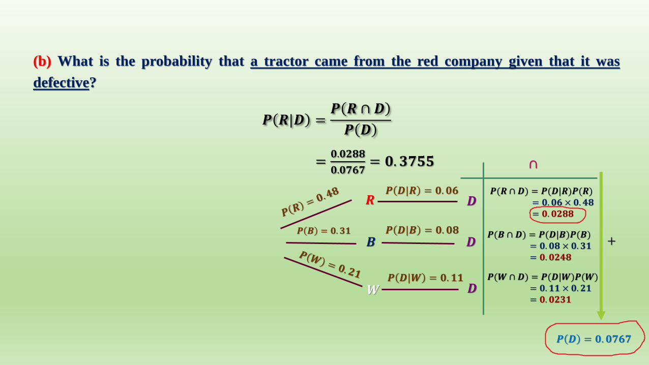
(b) What is the probability that a tractor came from the red company given that it was

defective?

𝑷 𝑹|𝑫 =𝑷 𝑹 ∩ 𝑫

𝑷 𝑫

=𝟎.𝟎𝟐𝟖𝟖

𝟎.𝟎𝟕𝟔𝟕= 𝟎. 𝟑𝟕𝟓𝟓

𝑹

𝑩

𝑾

𝑫

𝑫

𝑫

𝑷 𝑩 = 𝟎. 𝟑𝟏

𝑷 𝑫|𝑹 = 𝟎. 𝟎𝟔

𝑷 𝑫|𝑩 = 𝟎. 𝟎𝟖

𝑷 𝑫|𝑾 = 𝟎. 𝟏𝟏

∩

𝑷(𝑹 ∩ 𝑫) = 𝑷(𝑫|𝑹)𝑷(𝑹)= 𝟎. 𝟎𝟔 × 𝟎. 𝟒𝟖= 𝟎. 𝟎𝟐𝟖𝟖

𝑷(𝑩 ∩ 𝑫) = 𝑷(𝑫|𝑩)𝑷(𝑩)= 𝟎. 𝟎𝟖 × 𝟎. 𝟑𝟏= 𝟎. 𝟎𝟐𝟒𝟖

𝑷(𝑾∩𝑫) = 𝑷(𝑫|𝑾)𝑷(𝑾)= 𝟎. 𝟏𝟏 × 𝟎. 𝟐𝟏= 𝟎. 𝟎𝟐𝟑𝟏

+

𝑷 𝑫 = 𝟎. 𝟎𝟕𝟔𝟕

Sheet (3) [Revision on Probability]

2. A test for a rare disease claims that it will report a positive result for 99.5% of people with

the disease, and will report a negative result for 99.9% of those without the disease. We

know that the disease is present in the population at 1 in 100,000. Knowing this information,

what is the likelihood that an individual who tests positive will actually have the disease?

𝑫

𝑫′

Let:

The person with the disease: D.

The person without the disease: D′.

+𝒗𝒆∩

𝑷(𝑫 ∩ +𝒗𝒆) = 𝑷(+𝒗𝒆|𝑫)𝑷(𝑫)= 𝟎. 𝟗𝟗𝟓 × 𝟎. 𝟎𝟎𝟎𝟎𝟏= 𝟗. 𝟗𝟓 × 𝟏𝟎−𝟔

𝑷(𝑫 ∩ −𝒗𝒆) = 𝑷(−𝒗𝒆|𝑫)𝑷(𝑫)= 𝟎. 𝟎𝟎𝟓 × 𝟎. 𝟎𝟎𝟎𝟎𝟏= 𝟓 × 𝟏𝟎−𝟑

𝑷(𝑫′ ∩ +𝒗𝒆) = 𝑷(+𝒗𝒆|𝑫′)𝑷(𝑫′)= 𝟎. 𝟎𝟎𝟏 × 𝟎. 𝟗𝟗𝟗𝟗𝟗= 𝟗. 𝟗𝟗𝟗𝟗 × 𝟏𝟎−𝟒

−𝒗𝒆

−𝒗𝒆

+𝒗𝒆

𝑷(𝑫′ ∩ −𝒗𝒆) = 𝑷(−𝒗𝒆|𝑫′)𝑷(𝑫′)= 𝟎. 𝟗𝟗𝟗 × 𝟗𝟗𝟗𝟗𝟗= 𝟎. 𝟗𝟗𝟖𝟗𝟗𝟎𝟎𝟏

Note that:𝑃 𝐴|𝐸 + 𝑃 𝐵|𝐸 +⋯+ 𝑃 𝑍 𝐸= 1

what is the likelihood that an individual who tests positive will actually have the disease?

𝑷 𝑫| + 𝒗𝒆 =𝑷 𝑫 ∩ +𝒗𝒆

𝑷 +𝒗𝒆=

𝑷 𝑫 ∩ +𝒗𝒆

𝑷 𝑫 ∩ +𝒗𝒆 + 𝑷 𝑫′ ∩ +𝒗𝒆

=𝟗.𝟗𝟓×𝟏𝟎−𝟔

𝟗.𝟗𝟓×𝟏𝟎−𝟔 + 𝟗.𝟗𝟗𝟗𝟗×𝟏𝟎−𝟒= 𝟗. 𝟖𝟓𝟐𝟏 × 𝟏𝟎−𝟑 = 𝟎. 𝟎𝟎𝟗𝟖𝟓𝟐𝟏

𝑫

𝑫′

+𝒗𝒆∩

𝑷(𝑫 ∩ +𝒗𝒆) = 𝑷(+𝒗𝒆|𝑫)𝑷(𝑫)= 𝟎. 𝟗𝟗𝟓 × 𝟎. 𝟎𝟎𝟎𝟎𝟏= 𝟗. 𝟗𝟓 × 𝟏𝟎−𝟔

𝑷(𝑫 ∩ −𝒗𝒆) = 𝑷(−𝒗𝒆|𝑫)𝑷(𝑫)= 𝟎. 𝟎𝟎𝟓 × 𝟎. 𝟎𝟎𝟎𝟎𝟏= 𝟓 × 𝟏𝟎−𝟑

𝑷(𝑫′ ∩ +𝒗𝒆) = 𝑷(+𝒗𝒆|𝑫′)𝑷(𝑫′)= 𝟎. 𝟎𝟎𝟏 × 𝟎. 𝟗𝟗𝟗𝟗𝟗= 𝟗. 𝟗𝟗𝟗𝟗 × 𝟏𝟎−𝟒

−𝒗𝒆

−𝒗𝒆

+𝒗𝒆

𝑷(𝑫′ ∩ −𝒗𝒆) = 𝑷(−𝒗𝒆|𝑫′)𝑷(𝑫′)= 𝟎. 𝟗𝟗𝟗 × 𝟗𝟗𝟗𝟗𝟗= 𝟎. 𝟗𝟗𝟖𝟗𝟗𝟎𝟎𝟏