Comparison and Interpretation of Short-Term and Overall Indices

University of RichmondUR Scholarship Repository

Management Faculty Publications Management

2008

Capability Ratios: Comparison and Interpretationof Short-Term and Overall IndicesLewis A. LitteralUniversity of Richmond, [email protected]

Frank Rudisill

Follow this and additional works at: http://scholarship.richmond.edu/management-faculty-publications

Part of the Management Sciences and Quantitative Methods Commons, and the PerformanceManagement Commons

This Article is brought to you for free and open access by the Management at UR Scholarship Repository. It has been accepted for inclusion inManagement Faculty Publications by an authorized administrator of UR Scholarship Repository. For more information, please [email protected].

Recommended CitationLitteral, Lewis A. "Capability Ratios: Comparison and Interpretation of Short-Term and Overall Indices." International Journal ofQuality and Standards 2, no. 1 (2008): 67-86.

http://robins.richmond.edu/?utm_source=scholarship.richmond.edu%2Fmanagement-faculty-publications%2F50&utm_medium=PDF&utm_campaign=PDFCoverPages

http://robins.richmond.edu/?utm_source=scholarship.richmond.edu%2Fmanagement-faculty-publications%2F50&utm_medium=PDF&utm_campaign=PDFCoverPages

http://scholarship.richmond.edu?utm_source=scholarship.richmond.edu%2Fmanagement-faculty-publications%2F50&utm_medium=PDF&utm_campaign=PDFCoverPages

http://scholarship.richmond.edu/management-faculty-publications?utm_source=scholarship.richmond.edu%2Fmanagement-faculty-publications%2F50&utm_medium=PDF&utm_campaign=PDFCoverPages

http://scholarship.richmond.edu/management?utm_source=scholarship.richmond.edu%2Fmanagement-faculty-publications%2F50&utm_medium=PDF&utm_campaign=PDFCoverPages



http://network.bepress.com/hgg/discipline/637?utm_source=scholarship.richmond.edu%2Fmanagement-faculty-publications%2F50&utm_medium=PDF&utm_campaign=PDFCoverPages



mailto:[email protected]

Capability Ratios: Comparison and Interpretation of Short-Term and Overall Indices

Taken from The International Journal for Quality and Standards Page 1 of 20

Frank Rudisill, Lewis A. Litteral

CAPABILITY RATIOS: COMPARISON AND INTERPRETATION OF SHORT-TERM AND OVERALL INDICES

Frank Rudisill Management Department

School of Business Administration and Economics University of South Carolina Upstate

800 University Way Spartanburg, SC 29303

(864) 503-5511 [email protected]

and

Lewis A. Litteral * Management Department Robins School of Business

University of Richmond Richmond, VA 23173

(804) 289-8576 [email protected]

* Please send all correspondence to the second author.




CAPABILITY RATIOS: COMPARISON AND INTERPRETATION OF SHORT-TERM AND OVERALL INDICES

Keywords: Statistical process control, Capability indices

ABSTRACT

The ability of a process to satisfy customer requirements is frequently measured by capability

indices. The use and interpretation of these capability indices are often times misguided and or

misunderstood by those involved in this aspect of statistical process control. Those who monitor

and control processes and/or make decisions based on the reported values of these indices need

to have a clear understanding of indices that are reported by or to them. This paper addresses the

particular indices of Cp and Pp which indicate the capability of the process based only on its

variability and Cpk and Ppk which indicate process capability considering both variability and

location. A test is proposed to determine if there is significant non-common cause variability

and a method to estimate the unstable component of the overall variability is presented. A table

is provided to aid the analysis and examples based on the fiber characteristic of dyeability are

given.

Introduction

Many industries (automotive, paper, computer chips, paint, electronics, etc.) typically use

process capability indices to assess, monitor and communicate the capability of their processes




and products to meet tolerances/specifications. Capability assessment and improvement are

integral components of the ever-expanding Six Sigma philosophy (Breyfogle, 1999). Many

companies use these as the fundamental requirements for supplier selection and certification.

These indices also provide valuable internal information for setting priorities and identifying

processes that need improving.

There are many numerical ways to quantify capability of variables-type data. Some of the more

frequently used indices are; Cp, Cpk, Pp and Ppk. Each of these is defined carefully in the

following section. Computer software (Minitab, Statgraphics, Statistica, QI Analysis, and more)

calculates these as part of their capability analysis. Cp and Pp indicate the capability of

the process based only on its variability. Cpk and Ppk indicate process capability considering both

variability and location (average).

Bothe (1997) provides a comprehensive reference on process capability. He devotes a great deal

of discussion to the relationship between the Six Sigma philosophy and process capability

explaining that the often cited figure of 3.4 nonconformities per million opportunities is a result

of viewing the process as being dynamic rather than static and recognizing that small shifts in the

process average (less than +/ – 1.5 standard deviations) are often not detected. He provides

tables that relate values of capability indices to stated nonconformities per million opportunities.

For example, a Cp of 2.00 corresponds to a six sigma process when the process is dynamic. A

review of recent work on process capability indices appears in Kotz and Johnson (2002). There

is also an excellent series on the abuse and use of these indices in Gunter (1989a, b, c and d).




This paper proposes that practitioners who calculate, report and make decisions using these

capability indices first perform a statistical test (the F test) to determine if there is a statistically

significant component of non-common cause variability. If there is significant special cause

variability, we show how to estimate the unstable component and calculate the relative percent

contributions to the overall variability (this is useful in determining where to focus improvement

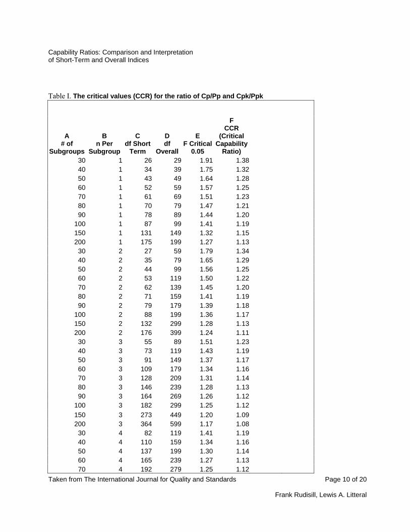
efforts). A table is presented showing the impact that sample size has on the estimates. Besides,

the use and interpretation of this procedure are illustrated with examples.

Some Capability Indices and their Estimates

Cp and Cpk reflect the capability of a process to meet specifications in the short run assuming the

process is stable.

Cp = (USL - LSL) /(3 σst) (1)

Cpk = min (Cpk upper, Cpk lower) where (2)

where

Cpk upper = (USL - μ)/ (3 σst) and (3)

Cpk lower = (μ - LSL)/(3 σst). (4)

USL = upper specification limit

LSL = lower specification limit

μ = process mean

σst = short term standard deviation of the process

μ is estimated with the following formula where k is the number of in-control subgroups;



= ==

Xk

K

ii∑

=

Χ1

__

. (5)

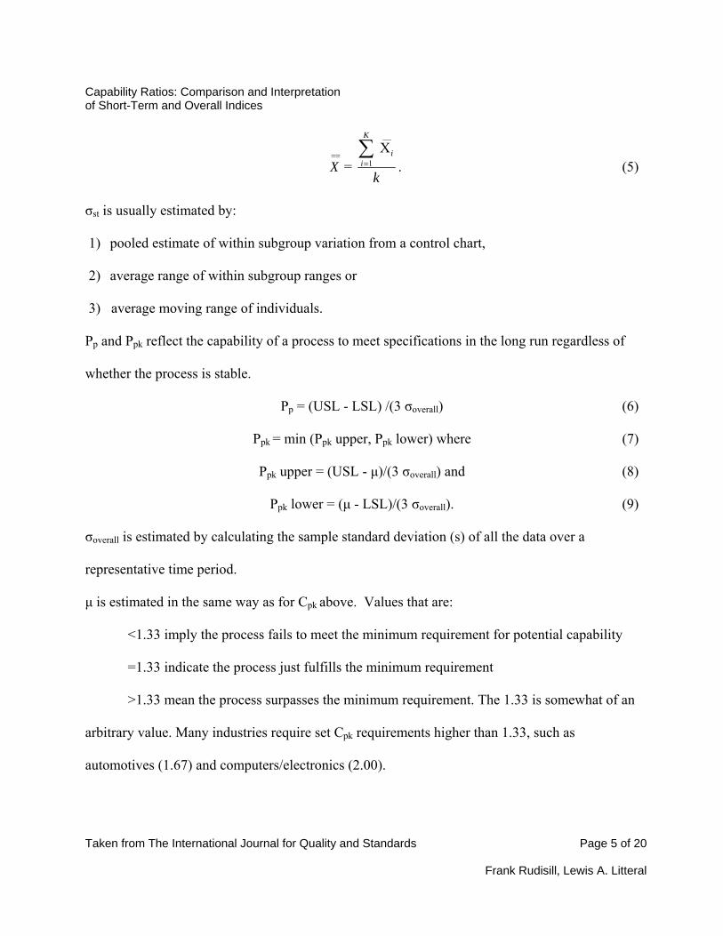
σst is usually estimated by:

1) pooled estimate of within subgroup variation from a control chart,

2) average range of within subgroup ranges or

3) average moving range of individuals.

Pp and Ppk reflect the capability of a process to meet specifications in the long run regardless of

whether the process is stable.

Pp = (USL - LSL) /(3 σoverall) (6)

Ppk = min (Ppk upper, Ppk lower) where (7)

Ppk upper = (USL - μ)/(3 σoverall) and (8)

Ppk lower = (μ - LSL)/(3 σoverall). (9)

σoverall is estimated by calculating the sample standard deviation (s) of all the data over a

representative time period.

μ is estimated in the same way as for Cpk above. Values that are:

<1.33 imply the process fails to meet the minimum requirement for potential capability =1.33 indicate the process just fulfills the minimum requirement >1.33 mean the process surpasses the minimum requirement. The 1.33 is somewhat of an

arbitrary value. Many industries require set Cpk requirements higher than 1.33, such as

automotives (1.67) and computers/electronics (2.00).




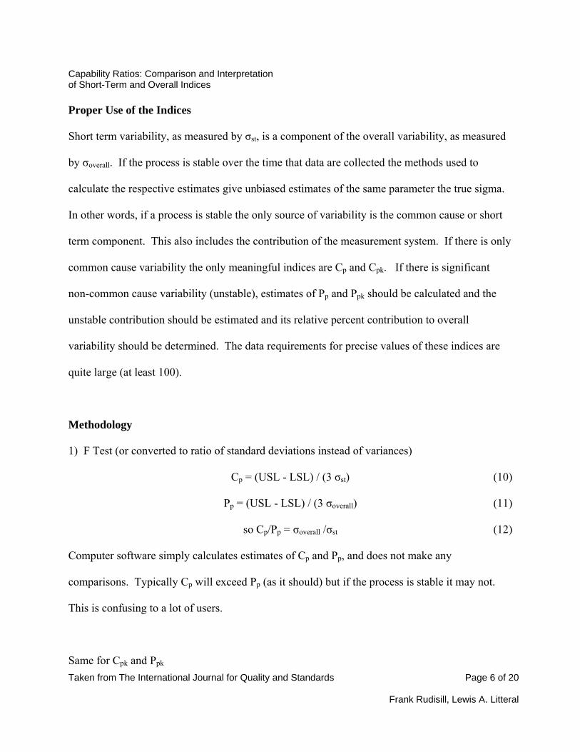
Proper Use of the Indices

Short term variability, as measured by σst, is a component of the overall variability, as measured

by σoverall. If the process is stable over the time that data are collected the methods used to

calculate the respective estimates give unbiased estimates of the same parameter the true sigma.

In other words, if a process is stable the only source of variability is the common cause or short

term component. This also includes the contribution of the measurement system. If there is only

common cause variability the only meaningful indices are Cp and Cpk. If there is significant

non-common cause variability (unstable), estimates of Pp and Ppk should be calculated and the

unstable contribution should be estimated and its relative percent contribution to overall

variability should be determined. The data requirements for precise values of these indices are

quite large (at least 100).

Methodology 1) F Test (or converted to ratio of standard deviations instead of variances)

Cp = (USL - LSL) / (3 σst) (10)

Pp = (USL - LSL) / (3 σoverall) (11)

so Cp/Pp = σoverall /σst (12)

Computer software simply calculates estimates of Cp and Pp, and does not make any

comparisons. Typically Cp will exceed Pp (as it should) but if the process is stable it may not.

This is confusing to a lot of users.

Same for Cpk and Ppk





Cpk/Ppk = σoverall /σst. (13)

This is intuitively appealing.

Thus, to determine if there is a statistical difference between Cp and Pp and Cpk and Ppk all we

have to do is to compare σoverall with σst.

Comparisons of variances (assuming the underlying populations are fairly normal) involve the F

ratio where the test statistic is the ratio of sample variances. The critical values found in an F

table depend upon the degrees of freedom of each sample variance.

Let k = the number of subgroups

and n = the number to samples within each subgroup.

The degrees of freedom for σoverall is nk-1, the degrees of freedom for σst is k(n-1) assuming σ 2st

is the pooled within subgroup variance. If the range method is used the degrees of freedom for

σst will be a different (less than) tabulated value. Also, if data are individuals, the 2 point

moving range is used to estimate σst. This situation is easily considered.

If the F stat does not exceed F critical we conclude that the only source of variability is short term

(common cause). That means the process is stable or in control. This should be evident in a

control chart. Recommend reporting Pp and Ppk as the measures of capability. Many companies

tend to misuse these statistics because they do not have adequate sample sizes. A general rule of




thumb is that the number of subgroups should be at least 100. With fewer than 100 subgroups

the estimates of σst and σoverall will be imprecise and could lead to either overstating or

understating capability.

2) Where is the variability?

If the Fstat exceeds the Fcritical there is statistically significant variability over and above the short

term variability.

a) This can be estimated by using the following formula and the respective estimates of the

variances.

σ 2 unstable = σ 2overall - σ 2st (14)

b) The percentage breakdowns are determined by:

stable % = σ 2st /σ 2overall *100% (15)

unstable % = σ 2 unstable / σ 2overall * 100% = 100% - stable %. (16)

These percentages are useful to management and quality engineers in setting priorities for

improvement. They indicate how successful the control plan is. If the unstable % is large (say

30 %) or more the control plan is not working.

The degrees of freedom for short term are based on using the ranges (or moving ranges) to

estimate sigma short term. One could also use the pooled estimates of within subgroup

variances.




In Table I, column F is the square root of column E. All one has to do is to divide Cp by Pp and

compare the result with column F. If the capability ratio is larger than the critical values in

column F there is significant unstable variability.




Table I. The critical values (CCR) for the ratio of Cp/Pp and Cpk/Ppk

A # of

Subgroups

B n Per

Subgroup

C df Short

Term

D df

Overall

E F Critical

0.05

F CCR

(Critical Capability

Ratio) 30 1 26 29 1.91 1.38 40 1 34 39 1.75 1.32 50 1 43 49 1.64 1.28 60 1 52 59 1.57 1.25 70 1 61 69 1.51 1.23 80 1 70 79 1.47 1.21 90 1 78 89 1.44 1.20

100 1 87 99 1.41 1.19 150 1 131 149 1.32 1.15 200 1 175 199 1.27 1.13

30 2 27 59 1.79 1.34 40 2 35 79 1.65 1.29 50 2 44 99 1.56 1.25 60 2 53 119 1.50 1.22 70 2 62 139 1.45 1.20 80 2 71 159 1.41 1.19 90 2 79 179 1.39 1.18

100 2 88 199 1.36 1.17 150 2 132 299 1.28 1.13 200 2 176 399 1.24 1.11

30 3 55 89 1.51 1.23 40 3 73 119 1.43 1.19 50 3 91 149 1.37 1.17 60 3 109 179 1.34 1.16 70 3 128 209 1.31 1.14 80 3 146 239 1.28 1.13 90 3 164 269 1.26 1.12

100 3 182 299 1.25 1.12 150 3 273 449 1.20 1.09 200 3 364 599 1.17 1.08

30 4 82 119 1.41 1.19 40 4 110 159 1.34 1.16 50 4 137 199 1.30 1.14 60 4 165 239 1.27 1.13 70 4 192 279 1.25 1.12




80 4 219 319 1.23 1.11 90 4 247 359 1.21 1.10

100 4 274 399 1.20 1.10 150 4 411 599 1.16 1.08 200 4 548 799 1.14 1.07

30 5 109 149 1.35 1.16 40 5 145 199 1.29 1.14 50 5 181 249 1.26 1.12 60 5 218 299 1.23 1.11 70 5 254 349 1.21 1.10 80 5 290 399 1.20 1.09 90 5 326 449 1.19 1.09

100 5 362 499 1.18 1.08 150 5 543 749 1.14 1.07 200 5 724 999 1.12 1.06

30 6 134 179 1.31 1.14 40 6 179 239 1.26 1.12 50 6 224 299 1.23 1.11 60 6 268 359 1.21 1.10 70 6 313 419 1.19 1.09 80 6 358 479 1.18 1.09 90 6 402 539 1.17 1.08

100 6 447 599 1.16 1.08 150 6 671 899 1.13 1.06 200 6 894 1199 1.11 1.05

*************** Source: Computations are based Wheeler (1990, p. 302)




Examples and Implications

The method described above is helpful to practitioners that use capability ratios to evaluate the

capability of their suppliers or their internal processes. The following examples illustrate the

application and interpretation of these ratios of capabilities ratios. The following data and

graphical examples are presented for illustrative purposes only. The data were generated via

computer simulation to reflect four different scenarios encountered by the authors in over 25

years of consulting experience. Fiber dyeability is used as the variable of interest, but this could

be any key process or product variable. Dyeability is a critical characteristic of fiber. Whether

the end product is automotive upholstery, residential or commercial carpet or apparel garments,

it is important that fiber producers control the dyeability of their materials. Fiber dyeability is

frequently measured and reported as a relative percentage of standard value. A 100% result

indicates that the production sample dyes the same as the reference standard. A 110% result

indicates that the production sample dyes 10% darker than the reference standard. Results less

than 100% indicate that the production sample dyes lighter than the standard.

In each of the following examples, the assumed customer requirements for fiber dyeability are

100% +/- 20% for each sample. The typical test protocol requires that four random samples

from each production run (lot) be samples and individually tested for dyeability.

Supplier A




Figure 1 shows the X-bar and R dyeability control charts based on the most recent 100 lots of

fiber produced by Supplier A. Note that both X-bar and R indicate that the dyeability is in

control. The estimated σst is 5.07 and the estimated σoverall is 5.12. Cp = 1.32 and Pp = 1.30.

The capability ratio is

Cp/Pp = Cpk/Ppk = σoverall /σst = 5.12/5.07 = 1.01. (17)

The critical ratio from Table 1 (with 100 subgroups of size 4) is 1.10. Thus, there is no

statistically significant special cause contribution to variability. Supplier A needs to maintain it’s

level of control and devote resources to reduce the common cause variability.

Supplier B

Now consider Supplier B’s X-bar and R charts as shown in Figure 2. Supplier B has several

points that indicate out-of-control conditions. The estimated σst is 5.07 (the same as Supplier A)

and the estimated σoverall is 5.66. Cp = 1.32 and Pp = 1.18.



This ratio is greater than the critical value of 1.10 in Table 1. Thus, there is a statistically

significant special cause contribution to variability.




The estimates of the percent contributions for stable and unstable components are:

stable % = σ 2st /σ 2overall *100% = 5.072/ 5.662 * 100% = 80%. (19)

unstable % = σ 2 unstable / σ 2overall * 100% = 100% - 80% = 20%. (20)

Thus, Supplier B’s special causes contribute 20% to his total variability. Supplier B needs to

reduce his common cause variability as well as improve his control system.

Supplier C

Next, consider Supplier C’s who has not devoted much attention to process control. Supplier C’s

X-bar and R charts are as shown in Figure 3. There are numerous indications of out-of-control

conditions. The estimated σst is 5.07 (the same as for Suppliers A and B) and the estimated σoverall

is 7.09. The results are Cp = 1.32 and Pp = 0.94, respectively.





Supplier C’s estimates of the percent contributions for stable and unstable components are:






Thus, Supplier C’s special cause contribution is half of his total variability. Supplier C definitely

needs to improve his control plan and then work to reduce his common cause variability.

Supplier D

To carry the example further, consider Supplier D’s X-bar and R charts as shown in Figure 4.

Supplier D is hard-pressed to find any points that indicate a stable condition. The estimated σst is

5.07 (the same as for Suppliers A, B and C) and the estimated σoverall is 9.00. Supplier D’s Cp =

1.32 (respectable) and Pp = 0.74 (disappointing).





The estimates of the percent contributions for D’s stable and unstable components are:






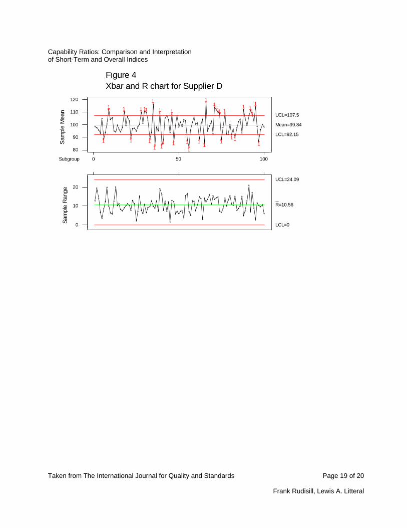
Thus, the majority of Supplier D’s variability is due to special causes. Supplier D needs to

significantly overhaul his control system since the current system is clearly not effective.

Discussion and Conclusion

The proposed method of calculating the ratios of capability indices, Cp and Pp, testing for

statistical significance and then estimating the relative percent contributions of common cause

and special cause variation is useful in a variety of scenarios by practitioners.

1. Process engineers may use this technique to evaluate their internal processes. If the F test

indicates statistically significant special cause variation then the control plan is not

effective and it should be improved. If the F test indicates no statistical significance, then

the Cp and Cpk values should be used to assess the need to reduce variation or center the

process (as they are intended).

2. This technique provides supply chain managers and engineers with a tool to evaluate

current and potential suppliers. If the F test indicates statistically significant special cause

variation then the supplier’s control plan is not effective. Procuring product from this

supplier may lead to problems even if the supplier reports capable Cp and Cpk values. If

the F test indicates no statistical significance, then the supplier has an effective control

plan and supplier capability can be evaluated based on the Cp and Cpk values.

The purpose of this paper was to present a method for comparing two routinely calculated

capability indices (Cp and Pp or Cpk and Ppk) and using this comparison to determine the

relative percent contributions of common and special causes to the total variability. The table

of critical ratios, the calculation of the percent contributions and the examples of four



supplier scenarios were presented to assist quality practitioners who frequently calculate the

ratios but are not sure of the best way to interpret and use them to improve their processes.

The techniques presented above are not stand alone methods. They should be used in

conjunction with other sound quality and process control techniques.

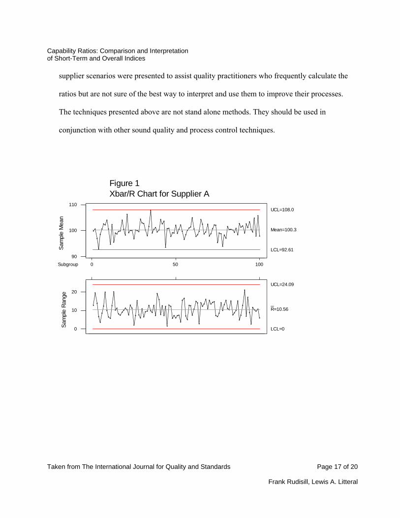
10050Subgroup 0

110

100

90

Sam

ple

Mea

n

Mean=100.3

UCL=108.0

LCL=92.61

20

10

0Sam

ple

Rang

e

R=10.56

UCL=24.09

LCL=0

Xbar/R Chart for Supplier AFigure 1




0Subgroup 50 10090

100

110

Sam

ple

Mea

n

Figure 2Xbar and R Chart for Supplier B

1

Mean=100.1

UCL=107.8

LCL=92.45


0

10

20

Sam

ple

Rang

e

R=10.56

UCL=24.09

LCL=0

0Subgroup 50 10085

95

105

115

Sam

ple

Mea

n

Figure 3

1 1 1

1

1

1 1 1 11

1 1

11

Xbar and R chart for SupplierC

1

Mean=100.0

UCL=107.7

LCL=92.301

1 1 1

0

10

20

Sam

ple

Rang

e

R=10.56

UCL=24.09

LCL=0



0Subgroup 50 100

80

90

100

110

120

Sam

ple

Mea

n

Figure 4Xbar and R chart for Supplier D


1

1 1

1

1 11

1

1

1

1

11

1

1 11

11

11111

1

1

11

1 11

Mean=99.84

UCL=107.5

LCL=92.15

1

1

0

10

20

Sam

ple

Rang

e

R=10.56

UCL=24.09

LCL=0




References

Bothe, Davis R., 1997. Measuring Process Capability: Techniques and Calculations for

Quality and Manufacturing Engineers. New York, NY: McGraw-Hill.

Breyfogle, Forrest W. III, 1999. Implementing Six Sigma. New York, NY: John Wiley & Sons, Inc. Gunter, Berton H., 1989a. The Use and Abuse of Cpk. Quality Progress, 72-73. Gunter, Berton H., 1989b. The Use and Abuse of Cpk. Part 2. Quality Progress, 108- 109. Gunter, Berton H., 1989c, The Use and Abuse of Cpk. Part 3. Quality Progress, 79- 80. Gunter, Berton H., 1989d, The Use and Abuse of Cpk. Part 4. Quality Progress, 86- 87. Kotz, Samuel and Johnson, Norman L., 2002. Process Capability Indices—A Review 1992-2000. Journal of Quality Technology, Vol. 34, No.1.

Wheeler, Donald J., 1990. Understanding Industrial Experimentation. Knoxville, TN: SPC

Press.

Date post:	07-Jan-2017
Category:	Documents
Upload:	lamtram
View:	216 times
Download:	1 times

Comparison and Interpretation of Short-Term and Overall Indices

Documents