Page 1
Comparison of 19 mm Superpave and
Marshall Base II Mixes
in West Virginia
John P. Zaniewski, Ph.D.
Vasavi Kanneganti
Asphalt Technology Program
Department of Civil and Environmental Engineering
Morgantown, West Virginia
June, 2003
Page 2
i
NOTICE
The contents of this report reflect the views of the authors who are responsible for
the facts and the accuracy of the data presented herein. The contents do not necessarily
reflect the official views or policies of the State or the Federal Highway Administration.
This report does not constitute a standard, specification, or regulation. Trade or
manufacturer names, which may appear herein, are cited only because they are
considered essential to the objectives of this report. The United States Government and
the State of West Virginia do not endorse products or manufacturers. This report is
prepared for the West Virginia Department of Transportation, Division of Highways, in
cooperation with the US Department of Transportation, Federal Highway Administration.
Page 3
ii
Technical Report Documentation Page
1. Report No. 2. Government
Accociation No.
3. Recipient's catalog No.
4. Title and Subtitle
Comparison of 19 mm Superpave and Marshall
Base II Mixes in West Virginia
5. Report Date June, 2003
6. Performing Organization Code
7. Author(s)
John P. Zaniewski, Vasavi Kanneganti 8. Performing Organization Report No.
9. Performing Organization Name and Address
Asphalt Technology Program
Department of Civil and Environmental
Engineering
West Virginia University
P.O. Box 6103
Morgantown, WV 26506-6103
10. Work Unit No. (TRAIS)
11. Contract or Grant No.
12. Sponsoring Agency Name and Address
West Virginia Division of Highways
1900 Washington St. East
Charleston, WV 25305
13. Type of Report and Period Covered
14. Sponsoring Agency Code
15. Supplementary Notes
Performed in Cooperation with the U.S. Department of Transportation - Federal Highway
Administration
16. Abstract
The WVDOH has implemented Superpave on all National Highway System projects
since 1997. The decision regarding implementation of Superpave for low volume roads in
WV is still under review. The primary objective of this research work was to compare the
19mm Superpave and Base II Marshall design mixes in WV to supplement information
required for WVDOH to make a suitable decision regarding the implementation of Superpave
for low volume roads.
The Marshall and Superpave methods were compared by preparing similar mix design
with each method. The mix designs from each method were cross-compared with the
conclusion that mixes developed under one method meet the criteria of the other method. In
addition, the Asphalt Pavement Analyzer (APA) was used to evaluate rutting performance of
gyratory compacted samples in the laboratory. The statistical analysis of rut depth results
indicated there is not enough evidence to conclude there is a significant difference between the
Marshall and Superpave mix design methods. It can be concluded that for the materials
evaluated in this research, the Marshall and Superpave methods produce interchangeable
results.
17. Key Words
Marshall, Superpave, Rutting Potential, Asphalt
mix design
18. Distribution Statement
19. Security Classif. (of this
report)
Unclassified
20. Security Classif. (of
this page)
Unclassified
21. No. Of Pages
77
22. Price
Form DOT F 1700.7 (8-72) Reproduction of completed page authorized
Page 4
iii
Table of Contents
CHAPTER 1 INTRODUCTION 1
1.1 INTRODUCTION 1
1.2 PROBLEM STATEMENT 1
1.3 OBJECTIVES 2
1.4 SCOPE OF WORK AND LIMITATIONS 2
1.5 REPORT OVERVIEW 3
CHAPTER 2 LITERATURE REVIEW 4
2.1 INTRODUCTION 4
2.2 MARSHALL MIX DESIGN 4
2.2.1 MATERIAL SELECTION 4
2.2.2 AGGREGATE GRADATION 5
2.2.3 SPECIMEN FABRICATION 6
2.2.4 VOLUMETRIC ANALYSIS 6
2.2.5 STABILITY AND FLOW MEASUREMENTS 7
2.2.6 OPTIMUM ASPHALT CONTENT 8
2.3 SUPERPAVE MIX DESIGN 9
2.3.1 GYRATORY COMPACTOR 9
2.3.2 MATERIAL SELECTION 10
2.3.3 DESIGN AGGREGATE STRUCTURE 11
2.3.4 DESIGN ASPHALT BINDER CONTENT 17
2.3.5 MOISTURE SENSITIVITY OF DESIGN MIXTURE 18
2.5 ASPHALT PAVEMENT ANALYZER 18
2.5.1 Evaluation of Permanent Deformation: 19
2.5.2 Results of Ruggedness Study of the APA 20
2.5.3 Effect of Compaction and Specimen Type 21
2.5.4 Effect of Position 21
2.6 Conclusions 21
CHAPTER 3 RESEARCH METHODOLOGY 23
3.1 INTRODUCTION 23
3.2 MATERIALS 23
3.3 AGGREGATE PREPARATION 23
Page 5
iv
3.4 SIEVE ANALYSIS 23
3.5 SPECIFIC GRAVITY OF AGGREGATES 24
3.6 AGGREGATE CONSENSUS PROPERTY TESTS 25
3.7 MARSHALL MIX DESIGN PROCEDURE 25
3.7.1 AGGREGATE GRADATION 26
3.7.2 SPECIFIC GRAVITY 26
3.7.3 THEORETICAL MAXIMUM SPECIFIC GRAVITY 27
3.7.4 MARSHALL STABILITY AND FLOW TEST 27
3.7.5 TABULATING AND PLOTTING TEST RESULTS 28
3.7.6 DETERMINATION OF DESIGN ASPHALT CONTENT 29
3.8 SUPERPAVE MIX DESIGN PROCEDURE 29
3.8.1 AGGREGATE TRIAL BLENDS 29
3.8.2 DESIGN AGGREGATE STRUCTURE 30
3.8.3 DESIGN ASPHALT CONTENT 33
3.9 SPECIMENS FOR APA TESTING 36
3.10 ASPHALT PAVEMENT ANALYZER RUNS 36
3.11 TESTs FOR OTHER CRITERIA 37
CHAPTER 4 RESULT AND ANALYSIS 38
CHAPTER 5 CONCLUSIONS AND RECOMMENDATIONS 41
5.1 CONCLUSIONS 41
5.2 RECOMMENDATIONS 41
5.3 FUTURE RESEARCH 42
REFERENCES 43
APPENDIX A AGGREGATE TESTS AND PROPERTIES 46
APPENDIX B Marshall Mix Design Data and Analysis 49
APPENDIX C Superpave Mix Design Data and Analysis 58
APPENDIX D Data and Analysis for Exchanging Superpave and Marshall Mix Designs68
List of Figures
Fig. 2.1 Superpave Gyratory Compactor 10
Figure 3.1 Marshall gradation plot with control points 26
Page 6
v
FIGURE 3.2 Superpave trial blend gradations 31
Fig 4.1 Output of Analysis of Variance 39
Figure B.1 Asphalt content versus Density – Marshall heavy 52
Figure B.2 Asphalt content versus Stability – Marshall heavy traffic mix. 52
Figure B.3 Asphalt content versus Flow – Marshall heavy traffic mix 53
Figure B.4 Asphalt content versus VTM – Marshall heavy traffic mix 53
Figure B.5 Asphalt content versus VMA – Marshall heavy traffic mix 54
Figure B.6 Asphalt content versus VFA –Marshall heavy traffic mix. 54
Figure B. 7 Asphalt content versus density, Marshall medium traffic mix. 55
Figure B.8 Asphalt content versus Stability – Marshall medium traffic mix. 55
Figure B.9 Asphalt content versus Flow – Marshall light traffic level 56
Figure B.10 Asphalt content versus Air voids –Marshall medium traffic mix. 56
Figure B.11 Asphalt content versus VMA – Marshall light traffic mix. 57
Figure B.12 Asphalt content versus VFA – Marshall 57
Figure C.1 Asphalt content versus Air voids-Superpave heavy traffic mix. 60
Figure C.2 Asphalt content versus VMA-Superpave heavy traffic mix. 60
Figure C.3 Asphalt content versus Percent Gmm at Nd-Superpave heavy traffic mix 61
Figure C.4 Asphalt content versus VFA – Superpave heavy traffic mix. 61
Figure C.5 Asphalt content versus Air voids-Superpave medium traffic mix. 63
Figure C.6 Asphalt content versus VMA-Superpave medium traffic level 63
Figure C.7 Asphalt content versus Percent of Gmm at Nd-Superpave medium traffic mix
64
Figure C.8 Asphalt content versus VFA-Superpave medium traffic mix. 64
Figure C.9 Asphalt content versus Air voids-Supeprave light traffic mix. 66
Page 7
vi
Fgure C.10 Asphalt content versus VMA-Superpave light traffic mix. 66
Figure C.11 Asphalt content versus percent Gmm at Nd-Supeprave light traffic mix. 67
Figure C.12 Asphalt content versus VFA - Superpave light traffic level 67
List of Tables
Table 2.1 Tolerance Limits of Master Gradation Range for Base II Mix-WVDOH
Standard Specifications 5
Table 2.2 Stability Correlation Ratios from AASHTO T245 8
Table 2.3 Marshall Mix Design Criteria (WVDOH MP 401.02.22). 9
Table 2.4 Superpave Aggregate Consensus Property Requirements as set forth by
WVDOH 12
Table 2.5 Gradation Specifications for 19mm Nominal Maximum Size 13
Table 2.6 Superpave Compaction Criteria (WVDOH MP 401.02.28) 15
Table 2.7 Superpave Volumetric Mix Design Criteria (WVDOH MP 401.02.28) 18
Table 2.8 APA Specifications (APAC Procedure) 20
Table 3.1 Washed Sieve Analysis for Material Passing #200 Sieve. 24
Table 3.2 Dry Sieve Gradation Analysis Results. 24
Table 3.3 Specific Gravity and Absorption Values. 24
Table 3.4 Average Consensus Property Test Results for Individual Aggregates 25
Table 3.6 Maximum Theoretical Specific Gravity for Marshall Mix Designs. 27
Table 3.7 Volumetric Parameters for Marshall Heavy Traffic Mix 28
Table 3.8 Volumetric Parameters for Marshall Medium Traffic Mix 28
Table 3.9 Summary of Marshall Mix Designs 29
Table 3.10 Trial Blends for Evaluation of Aggregate Structure 32
Table 3.11 Trial Blends Bulk and Apparent Specific Gravity 32
Page 8
vii
Table 3.12 Theoretical Maximum Specific Gravity for Superpave Trial Blends 32
Table 3.13 Trial Blends Compaction Data 32
Table 3.14 Adjusted Volumetric Parameters for Superpave Trial Blends 32
Table 3.15 Blend 1 Volumetric Parameters for Medium and Light Traffic Level Mix
Designs 33
Table 3.16 Adjusted Volumetric Parameters for Medium and Light Traffic Level Mix
Designs 33
Table 3.17 Average Gmm Values for Superpave Mixes 34
Table 3.18. Volumetric Data for Superpave Heavy Traffic Level. 34
Table 3.19 Volumetric Data for Superpave Medium Traffic Level 35
Table 3.20 Volumetric Data for Superpave Light Traffic Level 35
Table 3.21 Summary of Superpave Mix Designs. 35
Table 3.19 Treatments Used in Experimental Design 36
Table 3.20 Rut Depth Results. 37
Table 4.1 Confidence Interval Computed for Various Parameters 40
Table A.1 Gradation Data for Aggregates 46
Table A.2 Specific Gravity of Aggregates 47
Table A.3. Aggregate Consensus Property Tests 48
Table B.1 Theoretical Maximum Specific Gravity Calculations 49
Table B.2 Marshall Heavy Traffic Level Mix Design 50
Table B.3 Marshall Medium Traffic Mix Design 51
Table C.1 Theoretical Specific Gravity for Trial Blends 58
Table C.2 Bulk Specific Gravity for Trial Blends 58
Table C.3 Theoretical Maximum Specific Gravity Calculations for Superpave Heavy
Traffic Mix 59
Page 9
viii
Table C.4 Bulk Specific Gravity for Superpave Heavy Traffic Level Mix 59
Table C.5 Blend Bulk Specific Gravity Calculations –Superpave Medium Traffic Mix. 62
Table C.6 Theoretical Maximum Specific Gravity Calculations-Superpave Medium
Traffic Mix 62
Table C.7 Bulk Specific Gravity-Superpave Medium Traffic Mix. 62
Table C.8 Blend Bulk Specific Gravity Calculations –Superpave Light Traffic Mix. 65
Table C.9 Theoretical Maximum Specific Gravity Calculations-Superpave Light Traffic
Mix. 65
Table C.10 Bulk Specific Gravity-Superpave Light Traffic Mix. 65
Table D.1 Marshall Mix Designs with Superpave Methodology 68
Table D.2 Superpave Mix Designs with Marshall Methodology 69
Page 10
1
CHAPTER 1 INTRODUCTION
1.1 INTRODUCTION
Most hot mix asphalt (HMA) produced during the 50 years between the 1940s
and mid 1990s were designed using the Marshall or Hveem methods. Increases in traffic
volumes and heavier loads became initiative for the Strategic Highway Research Program
(SHRP) in 1988. After a five year of effort, a new mix design, Superior Performing
Asphalt Pavements (Superpave)TM
, was developed. Superpave takes into consideration
the factors that are responsible for the typical distresses on asphalt pavements: rutting,
fatigue and thermal cracking. With the introduction of Superpave mix design, the
Marshall method of mix design is becoming obsolete for highway pavements.
Superpave implementation varies by state. Some have completely switched over
to the national Superpave standards. Others have implemented the Superpave concepts,
but have adjusted criteria to suit local conditions. Others have partially implemented
Superpave for some projects but are using their legacy method for other projects. Finally,
two states, California and Nevada, are continuing to use legacy methods. The West
Virginia Division of Highways (WVDOH), constructed its first Superpave project on I-79
in 1997. Since then, WVDOH has implemented Superpave on all National Highway
System (NHS) projects. The decision regarding implementation of Superpave for
non-NHS roads in West Virginia is still under review. The primary objective of this
research work was to compare the Superpave and Marshall design mixes in West
Virginia to supplement information required for WVDOH to make a suitable decision
regarding the implementation of Superpave for low volume roads.
1.2 PROBLEM STATEMENT
One of the advantages of the Marshall mix design method in West Virginia is that
the performance of the mixes is known for local conditions and materials. There are no
Superpave projects for low volume roads in West Virginia to evaluate the performance of
mixes. An investigation is needed to compare the performance of Superpave and
Marshall mix design methods, to support replacement of conventional mix design with
the new mix design. This research work compared the Superpave and Marshall mixes in
Page 11
2
West Virginia using the Asphalt Pavement Analyzer (APA) to evaluate rutting
performance in the laboratory. Mix designs were prepared under the Marshall and
Superpave methodologies. The resulting Marshall mix designs were evaluated under the
Superpave criteria, and vice versa. If the mixes prepared under the Superpave method
met the Marshall criteria, it was hypothesized that these mixes would perform well in the
field. If the mixes prepared under the Marshall method pass the Superpave criteria, it was
hypothesized that contractors would not encounter any undue hardships in designing and
constructing pavements to the Superpave criteria.
1.3 OBJECTIVES
The objective of this research was to compare 19 mm Superpave and Base II
Marshall mixes in West Virginia. The primary area of interest for this comparison was
for medium and light traffic volume loads since the WVDOH has not implemented
Superpave for these traffic levels. The research included mix designs for high traffic
volume roads for completeness and to provide insight on how the research methodology
would rank these mixes.
1.4 SCOPE OF WORK AND LIMITATIONS
In this research work 19mm Superpave and Base II Marshall mixes were designed
for Heavy, Medium, and Light traffic levels. Marshall and Superpave mixes were
designed from locally available materials. The Marshall and Superpave mix design
procedures of the West Virginia Division of Highways (WVDOH) were followed.
Gyratory compactor was used to make the Asphalt Pavement Analyzer (APA) samples to
evaluate permanent deformation (rutting). Results from tests with different aggregates,
gradations, and binder types show that the APA is sensitive to these factors and,
therefore, has a potential to predict relative rutting of hot mix asphalt mixtures ( 2 ).
The experimental design used for this research work provides comparison
between the mixes, traffic levels and their interactions. The work was limited to Base-II
mixes in West Virginia and to one source of aggregate and asphalt cement. The 19mm
nominal maximum size aggregate was used for the two mix design methods. The J.F.
Page 12
3
Allen Company, Buckhannon, WV, provided the aggregate used for the research. The
asphalt used was PG 70-22 from the source Marathon Ashland.
The work was also limited to laboratory testing. Field evaluation could not be
performed since WVDOH has not constructed medium and light traffic volume
Superpave mixes.
1.5 REPORT OVERVIEW
This report is organized into five chapters and five appendices. After the first
chapter of Introduction, Chapter 2 is a summary of literature review. Superpave and
Marshall mix design procedures are outlined with standard test procedures and
specifications required by the WVDOH. The method of rut testing with the Asphalt
Pavement Analyzer (APA), as specified by the device manufacturer, is explained in
detail. The research methodology and procedures for preparing, testing and analyzing
samples is presented in Chapter 3. Chapter 4 presents the results of the experimental
design and the analysis of the results. Chapter 5 concludes the report with the
conclusions and recommendations.
The aggregate test data are presented in the Appendix A. Detailed test data and
interim calculations of Marshall and Superpave mix designs are presented in Appendix B
and Appendix C respectively. Appendix D presents the data for evaluating Superpave
mix design with Marshall methodology and vice versa.
Page 13
4
CHAPTER 2 LITERATURE REVIEW
2.1 INTRODUCTION
It was in 600’s B.C. that the first Asphalt road was paved in Babylon. The first
bituminous Hot Mix Asphalt (HMA) pavement in the United States was built in
Washington D.C, in 1873. In the years between the 1940s and mid 1990s, most of the
hot mix asphalt projects in United States were designed using the Marshall and Hveem
methods. According to survey in 1984, approximately 75 percent of the State Highway
Departments used some variation of the Marshall method while the remaining 25 percent
used some variation of Hveem method (4). In 1995, a few states began to use the
Superpave design procedures (4). The 2000 Superpave Implementation survey shows
that almost every state in United States is at some stage or the other in Superpave
implementation ( 8).
The Superpave and Marshall mix design methods, the Gyratory Compaction, and
Asphalt Pavement Analyzer (APA) are discussed in this chapter.
2.2 MARSHALL MIX DESIGN
Bruce Marshall, formerly the Bituminous Engineer with the Mississippi State
Highway Department, developed the original concept of the Marshall Method of
designing asphalt pavements. The present form of Marshall mix design method
originated from an investigation started by the U.S Army Corps of Engineers in 1943 (4).
The purpose of the Marshall method is to determine the optimum asphalt content for a
particular blend of aggregates and traffic level. The optimum asphalt content is
determined by the ability of a mix to satisfy stability, flow, and volumetric properties.
2.2.1 MATERIAL SELECTION
The materials used in the mix design should conform to the requirements set forth
in the Standard Specifications of WVDOH. Specifications for aggregate are covered
under sections 702 and 703 while asphalt cement is covered under section 705.
Page 14
5
2.2.2 AGGREGATE GRADATION
The aggregate blend gradation requirements for base II mixes is presented in
Table 2.1 (WVDOH Standard Specifications; Section 401). Aggregates meeting these
requirements are not placed in single stockpile, as this would promote segregation.
Therefore, stockpiles must be blended to meet the gradation specifications. Equation 2.1
is used to estimate the blended gradation from multiple stockpiles.
Table 2.1 Tolerance Limits of Master Gradation Range for Base II Mix-WVDOH
Standard Specifications
SIEVE BASE II
SIZE (mm) LEVEL
25 100
19 90-100
12.5 90 max
9.5
4.75
2.36 20-50
1.18
0.600
0.300
0.075 2.0-8.0
....CcBbAap (2.1)
where,
p = the percent of material passing a given sieve for the combined aggregates A, B, C….;
A, B, C,… = the percent of material passing a given sieve for each aggregate A, B, C,…;
a,b,c,… = proportions of aggregates A, B, C,… to be used in the blend.
The specific gravity for the blend is computed as:
n
n
n
G
P
G
P
G
P
PPPG
...
...
2
2
1
1
21 (2.2)
where,
Page 15
6
G = blend specific gravity;
G1, G2,…Gn = specific gravity values for fraction 1, 2,…n; and
P1, P2,…Pn = weight percentages of fraction 1,2,…n.
2.2.3 SPECIMEN FABRICATION
For determining the design asphalt content for a particular blend of aggregates by
the Marshall method, a series of test specimens are required to include a range of asphalt
contents of at least 2.0%, at intervals not to exceed 0.5%. Three specimens are required
for each asphalt content used in the design. The standard method for compacting the test
specimens is to immediately compact them after mixing process is completed. The
WVDOH requires that the specimens are oven aged for two hours. The WVDOH uses
compaction effort of 50 and 75 blows per side for medium and heavy traffic levels,
respectively. WVDOH uses the medium traffic level procedures for light traffic levels.
At least one specimen is required at the estimated asphalt content to determine the
maximum specific gravity (AASHTO T209). WVDOH requires two maximum specific
gravity samples. These samples are prepared at the estimated asphalt content for the mix.
2.2.4 VOLUMETRIC ANALYSIS
The bulk specific gravity of the compacted samples is measured and used with the
maximum theoretical specific gravity to perform the volumetric analysis. The volumetric
parameters and formulae for their calculation are:
sb
bmb
G
PGVMA
11100 (2.3)
1001mm
mb
G
GVTM (2.4)
100VMA
VTMVMAVFA (2.5)
where,
VMA = Volume of voids in mineral aggregate;
Page 16
7
Gmb = Bulk specific gravity of compacted mixture;
Pb = Asphalt content;
Gsb = Bulk specific gravity of aggregate;
VTM = Air voids in compacted mixture:
Gmm = Theoretical maximum specific gravity; and
VFA = Voids filled with asphalt.
Since the theoretical maximum specific gravity (Gmm) is only measured for one
asphalt content (preferably near the optimum), its value at the other asphalt contents is
computed as:
b
b
mm
bse
G
P
G
PG
1
1 (2.6)
b
b
se
b
mm
G
P
G
PG
''
'
1
1 (2.7)
where,
Gse = Effective specific gravity of aggregates;
Gmm = Theoretical maximum specific gravity measured;
Pb = Asphalt content used for Gmm samples;
'
mmG = Calculated theoretical maximum specific gravity;
'
bP = Asphalt content used for other compacted samples; and
Gb = Binder specific gravity (generally provided by binder supplier).
2.2.5 STABILITY AND FLOW MEASUREMENTS
Marshall stability is defined as the maximum load carried by a compacted
specimen tested at 140oF (60
oC) at a loading rate of 2 inches/minute ( 4). The flow is
measured at the same time as the Marshall stability. The flow is equal to the vertical
Page 17
8
deformation of the sample (measured from start of loading to the point at which stability
begins to decrease) in hundredths of an inch ( 4). The stability and flow measurements
procedure (AASHTO T245) indicates that the stability reading for a test specimen is only
accurate if the test specimen measures 63.5mm in height. For test specimens that vary
slightly from 63.5 mm, the stability reading should be multiplied with a correlation ratio
in Table 2.2 (AASHTO T245).
Table 2.2 Stability Correlation Ratios from AASHTO T245
Specimen Height Correlation Ratio
58.7 1.14
60.3 1.09
61.9 1.04
63.5 1.00
65.1 0.96
66.7 0.93
68.3 0.89
69.8 0.86
71.4 0.83
73.0 0.81
74.6 0.78
76.2 0.76
2.2.6 OPTIMUM ASPHALT CONTENT
The stability, flow, unit weight, air voids, VMA and VFA are plotted versus the
asphalt content. The optimum asphalt content of the mix is determined from the data
obtained from the plots. WVDOH specifies that the asphalt content that corresponds to
the specification’s median air void content (4.0%) is the optimum asphalt content. Using
the asphalt content at 4.0% air voids, the corresponding values for VMA, VFA, stability
and flow are determined from the plots and compared to the acceptance criteria in Table
2.3 (WVDOH MP 401.02.22). The mix must be redesigned using different aggregate
blends if design criteria are not satisfied.
Page 18
9
Table 2.3 Marshall Mix Design Criteria (WVDOH MP 401.02.22).
Design Criteria Medium traffic design Heavy traffic design
Compaction, number of
blows per side 50 75
Stability (Newton) 5300 8000
Flow (0.25 mm) 8-16 8-14
Air voids (%) 3-5 3-5
VFA, % 65-78 65-75
VMA, % 13* 13*
*VMA specifications are for Base II mix.
2.3 SUPERPAVE MIX DESIGN
Despite the best efforts put with the existing mix design methods, it is common to
see severe rutting and cracking in asphalt pavements due to increased traffic loads and
environmental conditions. In the 1988, a research program called Strategic Highway
Research Program (SHRP) was started in USA. The major funds of the SHRP research
program were allocated to establish new procedures for the selection of binders and mix
designs with regard to the rutting and cracking problems in the asphalt pavements. The
research program was completed in 1993, producing the Superpave mix design method
(7).
2.3.1 GYRATORY COMPACTOR
The key piece of equipment used in the Superpave mix design method is the
gyratory compactor, Figure 2.1. One of the main goals of the SHRP was to develop a
laboratory compaction method, which can consistently produce specimens representative
of in-service pavements. The Superpave gyratory compactor compacts HMA samples to
densities achieved under traffic loading conditions. Its ability to estimate specimen
density at any point during the compaction process is its key feature (4).
Gyratory compaction has been used in asphalt mix design since early 1900’s.
Midway through the Strategic Highway Research Program, an evaluation of available
gyratory compaction research was done to develop a gyratory protocol, which would
simulate the density achieved at the end of pavement’s life. Studies conducted during
SHRP show that the density of the HMA sample is influenced mostly by the angle of
Page 19
10
gyration, and slightly by the speed of gyration and the vertical pressure. The stresses
applied to the mixture and the mixture properties are the two parameters that would
influence asphalt mixture density (3).
Fig. 2.1 Superpave Gyratory Compactor
The AASHTO provisional standard TP 4-00 covers the compaction of cylindrical
specimens of hot-mix asphalt (HMA) using the Superpave gyratory compactor. This
standard specifies the compaction criteria of the Superpave gyratory Compactor. The
ram shall apply and maintain a pressure of 600 18 kPa perpendicular to the cylindrical
axis of the specimen during compaction. The compactor shall tilt the specimen at an
angle of 1.25 0.02 o and rotate the specimen molds at a rate of 30.0 0.5 gyrations per
minute throughout compaction.
The ruggedness evaluation of AASHTO TP4 conducted by FHWA arrived at the
conclusions that ( 9):
The tolerance on compaction angle ( 0.02o) is reasonable and necessary
The tolerance on compaction pressure ( 18kPa) is too high
2.3.2 MATERIAL SELECTION
Binder selection is based on environmental data, traffic level and traffic speed. A
Performance Grade asphalt binder is designated with a high and low temperature grade,
such as PG 70-22. For this binder, 70 is the high temperature grade and is the 7-day
maximum pavement design temperature in degrees centigrade for the project. The low
temperature grade, -22, is the minimum pavement design temperature in centigrade (5).
Page 20
11
The SHRP made no research effort to specifically look at aggregates. However,
guidance was eventually provided based on a consensus approach by a group of experts.
Superpave requires both consensus and source aggregate tests be performed to assure that
the combined aggregates selected for the mix design are acceptable. The consensus
property criteria are the minimum requirements for the aggregates to be used in the
Superpave mix design method and they are the same regardless of geographic location.
The source property criteria are specified by the state highway agencies (5). Superpave
requires the following consensus properties be determined for the design aggregate blend:
Coarse aggregate angularity (ASTM D 5821) –materials retained on 4.75 mm
sieve.
Fine Aggregate angularity (AASHTO T304) – materials passing the 2.36 mm
sieve.
Flat & Elongated particles (ASTM D4791) –materials retained on 9.5 mm
sieve.
Sand Equivalent (AASHTO T176) –materials passing the 4.75 mm sieve.
The flat and elongated test follows the general procedures of ASTM D 4791, but
is modified for Superpave. Under the Superpave guidelines an aggregate particle coarser
than 4.75mm sieve is flat and elongated if the ratio of the maximum to minimum
dimension is greater than 5 ( 5).
Aggregate property requirements set forth by WVDOH is shown in Table
2.4(WVDOH MP-2)
2.3.3 DESIGN AGGREGATE STRUCTURE
Trial blends are established by mathematically combining the gradations of
individual stockpiles into a single blend using Equation 2.1. The gradation of the
aggregate blend must be within the control limits to meet the Superpave requirements.
The gradation control is based on four control sieves: the maximum sieve, the nominal
Page 21
12
Table 2.4 Superpave Aggregate Consensus Property Requirements as set forth by
WVDOH
Design
ESALs
Coarse Aggregate
angularity (%min)*
Fine aggregate
angularity (%min)
Sand
equivalent
Flat &
elongated
(Million) 100 mm
from
surface
>100 mm
from
surface
100 mm
from
surface
>100 mm
from
surface
Percent
minimum
Percent
minimum
<0.3 55/- - - - 40 -
0.3 to <3 75/- 50/- 40 40 40 10
3 to <10 85/80 60/- 45 40 40 10
10 to <20 90/95 80/75 45 40 45 10
20 to <30 95/90 80/75 45 40 45 10
30 100/100 100/100 45 45 50 10
*Percent of one/more than one fractured faces
maximum sieve, the 2.36-millimeter sieve, and the 75-micron sieve. The Superpave
definitions for nominal maximum aggregate size and maximum aggregate size are:
Nominal Maximum Aggregate Size: One sieve size larger than the first sieve
to retain more than 10.0% of the material.
Maximum Aggregate Size: One sieve size larger than the nominal maximum
aggregate size.
The restricted zone is another part of grading specification. Aggregate blends that
pass through the restricted zone that do not use excessive amounts of rounded aggregates
and that meet the minimum VMA requirements perform satisfactorily (4). However, the
WVDOH specifications do not allow any mix with a gradation passing through the
restricted zone. There is evidence to support the belief that mixtures closer to the low
end of the control limits (those going underneath the restricted zone) provide a desirable
structure for resisting rutting ( 4). WVDOH Specifications for 19mm nominal maximum
size are shown in Table 2.5.
Once an aggregate blend is identified, which meets the gradation criteria, the
consensus propery for the blend is determined as:
...
...
2211
222111
pPpP
pPxpPxX (2.8)
Page 22
13
Table 2.5 Gradation Specifications for 19mm Nominal Maximum Size
SIEVE CONTROL POINTS RESTRICTED ZONE
SIZE
(mm)
Lower Upper Lower Upper
25 100 100 - -
19 90 100 - -
12.5 - 90 - -
9.5 - - - -
4.75 - - - -
2.36 23 49 34.6 34.6
1.18 - - 22.3 28.3
0.6 - - 16.7 20.7
0.3 - - 13.7 13.7
0.15 - - - -
0.075 2 8 - -
where
X = Blended consensus property;
xi = Consensus property for stockpile;
Pi = Percent of stockpile i in the blend; and
pi = Percent of stockpile which either passes or is retained on the dividing sieve.
The Superpave process requires evaluating the aggregate blends to determine a
design aggregate structure. The Superpave guidelines suggest selecting two blends with
gradation below the restricted zone and one blend with a gradation above the restricted
zone. The asphalt content for the blends may be estimated based on experience or using
the equations:
sbsasbse GGFGG (2.9)
sasb
se
s
b
b
as
baGG
G
P
G
P
VPV
111
(2.10)
nbe SV ln0675.0176.0 (2.11)
Page 23
14
se
s
b
b
as
s
G
P
G
P
VPW
1 (2.12)
sbabeb
babebbi
WVVG
VVGP (2.13)
where,
Gse = Effective specific gravity of aggregate;
Gsb = Bulk specific gravity of aggregate;
Gsa = Apparent specific gravity of aggregate;
F = factor for absorption;
Vba = volume of absorbed binder;
Pb = Asphalt content, percent by weight of mix;
Pc = percent of aggregate;
Gb = Specific gravity of binder;
Va = volume of air voids;
Ws = weight of aggregate;
Vba = volume of absorbed binder;
Vbe = volume of effective binder;
Sn = nominal maximum sieve size of aggregate blend; and
Pbi = percent (by weight) of binder;
Two samples are prepared for each aggregate blend. The samples are mixed,
cured for 2 hours and compacted and the Gmb is determined. The Superpave gyratory
compactor is used to compact the samples. The number of gyrations applied to the mix
regulates the compactive effort. The number of gyrations required is a function of the
traffic level. As shown in the Table 2.6, Superpave defines three compaction
requirements for a mix.
Page 24
15
Table 2.6 Superpave Compaction Criteria (WVDOH MP 401.02.28)
ESALs (million) Compaction Parameters
Ni Nd Nm
<0.3 6 50 75
0.3 to <3 7 75 115
3 to <30 8 100 160
> 30 9 125 205
The number of gyrations for design, Nd, was selected to simulate the compacted
state of an asphalt pavement following construction. An initial compactive effort, Ni,
was defined to identify “tender” mixes. Some mixes are difficult to compact in the field
because the mix lacks the internal friction required to prevent the excessive deformation.
As traffic is applied to a pavement, the mix will continue to compact until an equilibrium
condition is achieved. The maximum Superpave compactive effort, Nmax was selected to
ensure the material does not over compact under traffic. Nmax and Ni are a function of Nd:
Ni = (Nd)0.45
(2.14)
Nmax = (Nd)1.10
(2.15)
where
Ni = Initial number of gyrations;
Nd = Design number of gyrations; and
Nm = maximum number of gyrations.
The WVDOH requirements for compactive effort are given in Table 2.6.The
design aggregate structure samples are compacted to Nd. The bulk specific gravity of the
mix at Ni must be computed as:
di Nmb
i
dNmb G
h
hG ,, (2.16)
where
Gmb,Ni = Bulk specific gravity at Ni;
hd = Height of the specimen at Nd;
Page 25
16
hi = Height of the specimen at Ni;
Gmb,Nd = Bulk specific gravity at Nd;
The percent maximum specific gravity at Ni is computed as:
mm
Nmb
NmmG
GG i
i
,
, 100% (2.17)
Two samples for each aggregate blend are prepared and evaluated to determine
Gmm. Gmb and Gmm are used for a volumetric analysis. VTM, VMA and VFA are
computed using equations 2.3 to 2.5.
Since Pb was only estimated, the VTM is generally not equal to the criteria of
4.0% air voids. Thus, the volumetric parameters are “corrected” to a 4.0% air content
using the equations:
dabtestb NVPP @44.0, (2.18)
dadest NVCNVMAVMA @4@ (2.19)
estdaestest VMANVVMAVFA @100 (2.20)
daimmimm NVGGEst @0.4%% ,, (2.21)
dammmmmm NVGGEst @0.4%% ,, (2.22)
where
Pb,est = Estimated asphalt binder content;
Pbt = Trial percent asphalt binder content;
Va = percent air voids in total mix at Nd;
VMAest = Estimated voids in mineral aggregate;
C = 0.1 when Va is less than 4.0%,
C = 0.2 when Va is 4.0% or greater
VFAest = Estimated voids filled with asphalt;
Page 26
17
Est%Gmm,i = Estimated percentage of maximum specific gravity at Ni;
Est%Gmm,m = Estimated percentage of maximum specific gravity at Nd;
In addition the dust to binder ratio is computed as:
estb
sbse
sbsebsestbe P
GG
GGGPP ,,
(2.23)
estbe
mm
estbeP
PPF
,
075.0
,
%/ (2.24)
where
F/Pbe,est = Estimated fines to effective asphalt ratio; and
%P0.075mm = percent material finer than 0.075 mm sieve.
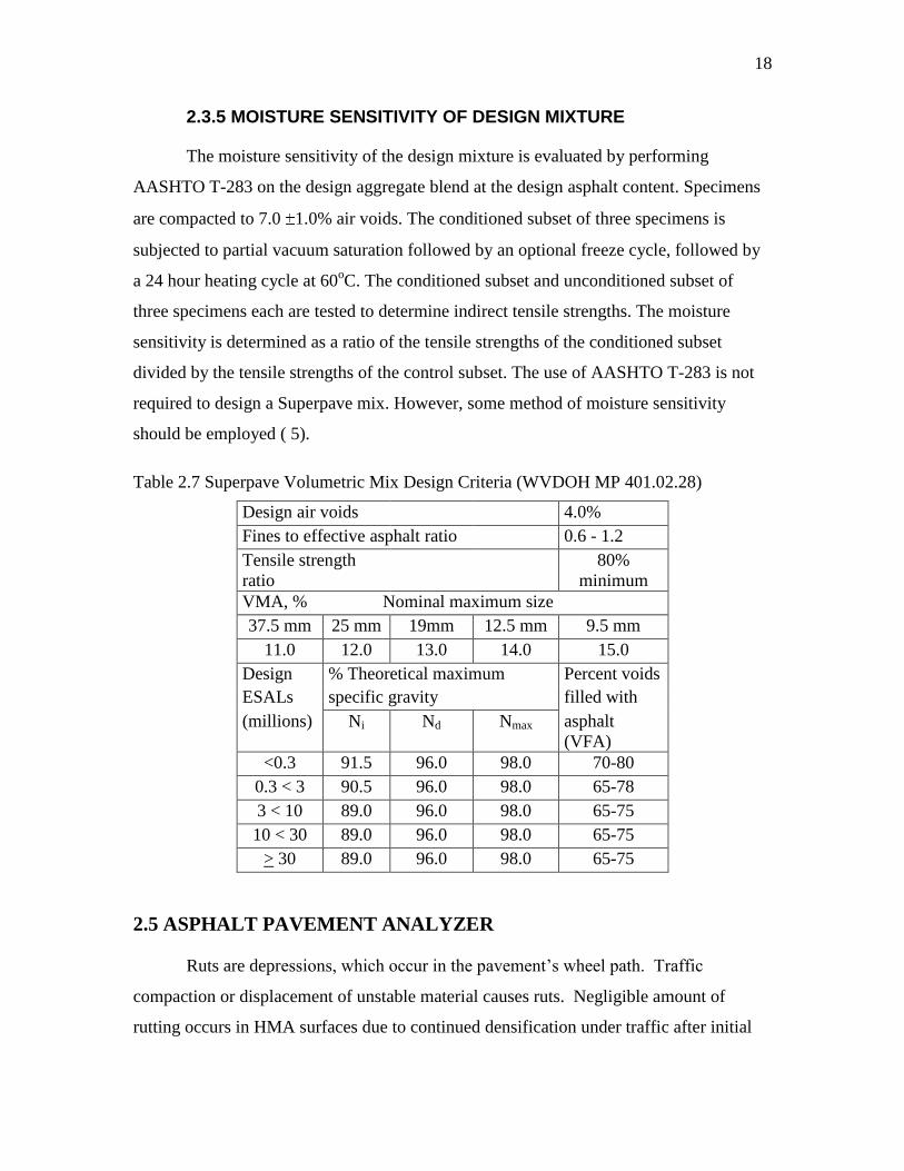
The corrected volumetric parameters are compared to the Superpave criteria,
Table 2.7. The design aggregate structure, which “best” meets the criteria is selected for
determining the design binder content. If none of the aggregate blends produce an
acceptable mix, a new aggregate blend must be determined and evaluated.
2.3.4 DESIGN ASPHALT BINDER CONTENT
The design binder content is defined by Superpave as the asphalt content that
produces 4.0% air voids at Nd and meets all other criteria. A good estimate of design
asphalt content is established from the design aggregate blend trials. Two or three
samples depending on the agency are prepared at four levels of binder content:
Pb,est-0.5%, Pb,est, Pb,est +0.5% and Pb,est+1.0%. The samples are compacted to Nd
gyrations and a volumetric analysis is performed and the results are plotted. As with the
Marshall procedure, the asphalt content corresponding to 4.0% air voids is determined.
This asphalt content is used with other plots to determine the other volumetric properties.
The design mixture must meet the requirements for Ni, VMA, VFA and dust to binder
ratio as presented in Table 2.7. Two additional samples are mixed with the selected
asphalt content and compacted to Nm to verify the mix meets the criteria.
Page 27
18
2.3.5 MOISTURE SENSITIVITY OF DESIGN MIXTURE
The moisture sensitivity of the design mixture is evaluated by performing
AASHTO T-283 on the design aggregate blend at the design asphalt content. Specimens
are compacted to 7.0 1.0% air voids. The conditioned subset of three specimens is
subjected to partial vacuum saturation followed by an optional freeze cycle, followed by
a 24 hour heating cycle at 60oC. The conditioned subset and unconditioned subset of
three specimens each are tested to determine indirect tensile strengths. The moisture
sensitivity is determined as a ratio of the tensile strengths of the conditioned subset
divided by the tensile strengths of the control subset. The use of AASHTO T-283 is not
required to design a Superpave mix. However, some method of moisture sensitivity
should be employed ( 5).
Table 2.7 Superpave Volumetric Mix Design Criteria (WVDOH MP 401.02.28)
Design air voids 4.0%
Fines to effective asphalt ratio 0.6 - 1.2
Tensile strength
ratio
80%
minimum
VMA, % Nominal maximum size
37.5 mm 25 mm 19mm 12.5 mm 9.5 mm
11.0 12.0 13.0 14.0 15.0
Design % Theoretical maximum Percent voids
ESALs specific gravity filled with
(millions) Ni Nd Nmax asphalt
(VFA)
<0.3 91.5 96.0 98.0 70-80
0.3 < 3 90.5 96.0 98.0 65-78
3 < 10 89.0 96.0 98.0 65-75
10 < 30 89.0 96.0 98.0 65-75
> 30 89.0 96.0 98.0 65-75
2.5 ASPHALT PAVEMENT ANALYZER
Ruts are depressions, which occur in the pavement’s wheel path. Traffic
compaction or displacement of unstable material causes ruts. Negligible amount of
rutting occurs in HMA surfaces due to continued densification under traffic after initial
Page 28
19
compaction during construction. Rutting in a pavement can be larger if the HMA layer,
underlying layers, or the subgrade soil is overstressed and significant densification or
shear failures occur. Some common mistakes made when designing the HMA mixes like
selection of high asphalt content, use of excessive filler material (material passing #200
sieve), use of too many rounded particles in aggregates are all contributors to rutting in
HMA ( 4). In recent years, the potential for rutting on the nation’s highways has
increased due to higher traffic volumes and the increased use of radial tires that typically
exhibit higher inflation pressures ( 6).
The most common type of laboratory equipment that predicts field-rutting
potential is a loaded wheel tester (LWT). The LWTs currently being used in United
States include the Georgia Loaded Wheel Tester (GLWT), Asphalt pavement Analyzer
(APA), Hamburg Wheel Tracking Device (HWTD), LCPC (French) Wheel Tracker,
Purdue University Laboratory Wheel Tracking Device (PURWheel), and one-third scale
Model Mobile Load Simulator ( 6).
The APA is the new generation of the Georgia Loaded GLWT and was first
manufactured in 1996 by Pavement Technology, Inc. The APA is a multi-functional
LWT that can be used for evaluating rutting, fatigue cracking, and moisture susceptibility
of hot and cold asphalt mixes (2).
2.5.1 Evaluation of Permanent Deformation:
The standard method followed to determine rutting susceptibility using APA is
developed by APAC Materials Services in ASTM format. Rutting susceptibility of mixes
is estimated by placing beam or cylindrical samples under repetitive wheel loads and
measuring the amount of permanent deformation under the wheel loads. Triplicate beam
samples or cylindrical samples can be tested in APA under controllable high temperature
and in dry or submerged-in water conditions. The rut depth is measured after the desired
number of cycles (usually 8000) of load application (11). The Table 2.8 shows the test
parameters specified in the APAC procedure.
Page 29
20
Table 2.8 APA Specifications (APAC Procedure)
Factors Range specified in
APAC procedure
Air void content 7 1 %
Test
temperature
Based on average
high pavement
temperature
Wheel load 100 5 lb
Hose pressure 100 5 psi
Specimen type Beams, cylinders
Compaction Rolling, vibratory,
and gyratory
2.5.2 Results of Ruggedness Study of the APA
APAC Materials Services conducted a ruggedness study of the Asphalt Pavement
Analyzer rutting test in 1999 ( 11). Six factors; air void content of the test specimens, the
test temperature, specimen preheating time, wheel load, hose pressure, and specimen
compaction method were investigated and the following conclusions and
recommendations were made regarding the specifications of the standard procedure.
1. The air void content range of the specimens given in the procedure should be
changed from 7 1.0% to 7 0.5%. This will reduce the variability in the test
results but it will also affect the productivity of the labs because of having to
discard samples out of the tighter range.
2. The test temperature has a major effect on the test results. Proper calibration
of the APA chamber temperature and ovens for preheating specimens is
critical in obtaining meaningful test results.
3. Compaction and specimen type had a significant effect on the test results.
4. The ranges evaluated in the study for preheat time, wheel load, and the hose
pressure did not have a significant effect on the rut results. Therefore, it was
concluded that the standard procedure gives adequate guidance on the control
of each of these test parameters.
Page 30
21
2.5.3 Effect of Compaction and Specimen Type
The results from the ruggedness study of the APA shows that for the low rut
potential mixes, the Superpave Gyratory Compactor (SGC) cylinders tended to have
higher rut depths, while for the high rut potential mixes the Asphalt Vibratory Compactor
(AVC) beams yielded collectively higher rutting. The reasons postulated for this behavior
are:
In high rut potential mixes, the center part of the cylinder mold supports the
load when the rut depth advances to the depth of the contour at the center of
the mold (12).
The compaction modes of cylinder and beam samples may produce different
density gradients in the samples (12).
The evaluation of density gradients in APA samples shows that vibratory
compaction tends to result in more compaction at the top and less compaction at the
bottom for both beams and cylinders. Gyratory compacted samples showed less
compaction in the top and bottom of samples and significantly more compaction in the
middle. The top of the AVC specimens should be loaded in APA. This type of
specification is not needed for SGC compacted samples as the density in the top and
bottom layers were not significant not significantly different (12).
2.5.4 Effect of Position
Studies have shown that there is variation in the left, center and right rut depth
measurements of the APA. Although the wheel loads are individually calibrated, it has
been observed that the wheel loads are not necessarily independent. During calibration,
the load applied by any wheel is affected by whether or not the other wheels are in
loading or rest position indicating the is an interaction between the wheel loads.
2.6 CONCLUSIONS
The Marshall and Superpave mix design methods were briefly described. State
highway agencies have some discretion in the specific details of how the methods are
implemented. The specifics for the WVDOH method were presented since they are the
methods and procedures followed during this research.
Page 31
22
The literature on the APA demonstrates it is a useful device for evaluating the
rutting potential of a mix. However, there is an inherent variability in the results
produced with the device, particularly with respect to load position. The experimental
plan developed for this research was designed to minimize the effect of the variability in
the APA results.
Page 32
23
CHAPTER 3 RESEARCH METHODOLOGY
3.1 INTRODUCTION
This research compares 19 mm nominal maximum aggregate size Superpave to
Marshall Base II mixes in West Virginia. Mix designs were prepared for Heavy, Medium
and Light traffic levels using the Superpave methodology and for Heavy and Medium
traffic level using the Marshall methodology. The resulting Marshall mix designs were
evaluated under the Superpave criteria and vice versa. APA samples were made using
Gyratory Compactor to evaluate rutting potential of the mixes. The following sections of
this chapter explain the laboratory-testing program conducted in the Asphalt Technology
Laboratory of West Virginia University, Morgantown. The data and interim calculations
for the aggregates are presented in Appendix A.
3.2 MATERIALS
The aggregate used in this research work was provided by J.F Allen Company,
Buckhannon, WV. Four types of aggregates (#57, #8, #9, Limestone Sand) and bag fines
were used to develop aggregate blends meeting the gradation requirements. The asphalt
used for both Superpave and Marshall mix design methods was PG 70-22 obtained from
Marathon, Ashland.
3.3 AGGREGATE PREPARATION
The aggregates were obtained from J.F. Allen Company. Three of the aggregate
types were ASTM coarse aggregate sizes #57, #8, and #9. The fourth aggregate type was
crushed limestone sand. The aggregates were processed by washing, oven drying and
sieving. Dried aggregates were separated with a nest of sieves, consisting of: 1”, 3/4”,
3/8”, #4, #8, #16, #30, #50, and #200 and the material retained on each sieve and pan
was placed in storage bins.
3.4 SIEVE ANALYSIS
Three samples of each aggregate type were tested to determine the amount of
material passing the #200 sieve (ASTM C117) and to determine gradation (ASTM
C136). The amount of material passing the #200 sieve was determined by washed
Page 33
24
sieving for each type of aggregate is shown in Table 3.1. The average gradation results
for each aggregate type are shown in Table 3.2.
Table 3.1 Washed Sieve Analysis for Material Passing #200 Sieve.
Sample No. #57 #8 #9 L. Sand
1 0.9 1.3 1.3 6.9
2 0.9 2.0 1.5 6.7
3 1.1 1.2 1.9 6.4
Average 1.0 1.5 1.6 6.7
Table 3.2 Dry Sieve Gradation Analysis Results.
Sieve No. Sieve size #57 #8 #9 Limestone Sand Bag fines
% passing % passing % passing % passing %passing
1” 25 mm 100 100 100 100 100
¾” 19 mm 84 100 100 100 100
3/8” 12.5 mm 36 100 100 100 100
½” 9.5 mm 14 96 100 100 100
#4 4.75 mm 2.4 14 69 99 100
#8 2.36 mm 1.6 3.5 5.0 77 100
#16 1.18 mm 1.4 2.3 2.1 45 100
#30 0.6 m 1.3 1.9 1.9 29 100
#50 0.3 m 1.2 1.7 1.8 17 97.0
#200 0.075 m 1.0 1.5 1.7 6.6 92.0
3.5 SPECIFIC GRAVITY OF AGGREGATES
Three samples of each aggregate type and one sample of bag fines were tested to
determine the specific gravity and absorption (AASHTO T85 for coarse aggregate
AASHTO T84 for fine aggregate). The average specific gravity and absorption values
are shown in Table 3.3.
Table 3.3 Specific Gravity and Absorption Values.
#57 #8 #9 L. sand Bag
Fines
Bulk Specific Gravity 2.687 2.686 2.648 2.665
Apparent Specific Gravity 2.731 2.734 2.751 2.732 2.680
% Absorption 0.6 0.7 1.4 0.9
Page 34
25
3.6 AGGREGATE CONSENSUS PROPERTY TESTS
The aggregate properties that are specified as a result of the SHRP program are
the coarse and fine aggregate angularity, flat and elongated particles, and sand equivalent
results. Three samples each of #57 and #8 aggregate were tested to determine the average
coarse aggregate angularity ( ASTM D5821). Three samples each of #8, #9 and
Limestone Sand were tested to determine the Uncompacted Void Content of Fine
Aggregate (AASHTO T304 Method A). Following the general procedures of ASTM D
4791, three samples of #57 and #8 aggregate were tested to determine the average Flat
and Elongated particles whose maximum to minimum dimension is greater than 5. Three
samples of Limestone Sand were tested to get an average sand equivalent value
(AASHTO T176). The aggregate average consensus property test results are shown in
Table 3.4. The aggregate blends met the Superpave mix design criteria.
Table 3.4 Average Consensus Property Test Results for Individual Aggregates
Property #57 #8 #9 L.Sand
Coarse aggregate angularity 100/100 100/100
Fine aggregate angularity 46.0 46.0 46.0
Flat & elongated particles 0 0
Sand equivalent value 100 78.0
3.7 MARSHALL MIX DESIGN PROCEDURE
The design traffic levels used in Marshall mix design method were Medium
Traffic (less than 3 million ESALs), and Heavy Traffic (greater than 3 million ESALs).
The binder used in the mix design was PG 70-22 (obtained from the source
Marathon/Ashland). The aggregate in the storage bins were combined as required to
produce the required gradation. The steps followed in determining the two Marshall mix
designs are explained in the following section. The summary of the tests performed in
determining the Marshall mixes are presented in this section. The detailed test data and
calculations are presented in Appendix B.
Page 35
26
3.7.1 AGGREGATE GRADATION
The result of sieve analysis of aggregates shown in Table 3.2 were used to
combine the aggregate to achieve an aggregate blend used by J.F. Allen Company for
Marshall Base II mix:
Aggregate type Percent of
blend
#57 35.5
#8 17.0
#9 10.0
Sand 36.5
Bag house fines 1.0
The plot of gradation is shown in Figure 3.1 with control points. The aggregate
blend was within the tolerance limits of Master Range and hence the aggregate structure
meets the gradation requirements; Table 2.4
Figure 3.1 Marshall gradation plot with control points
3.7.2 SPECIFIC GRAVITY
The binder supplier provided the specific gravity of the asphalt binder and the
value used was 1.020. The Equation 2.1 was used to calculate the specific gravity of the
Control points
Sieve size, mm
Per
cent
Pas
sing
Page 36
27
aggregate blend. The bulk specific gravity was 2.670 and the apparent specific gravity
was 2.733 for the blend.
3.7.3 THEORETICAL MAXIMUM SPECIFIC GRAVITY
From the experience of J.F.Allen Company, the optimum asphalt content for Base
II Marshall mix in West Virginia was 4.9% for Heavy traffic level. As described in
Chapter 2, the maximum theoretical specific gravity is measured at one asphalt content
and used to compute Gmm at the other asphalt contents. The validity of this approach
was tested by performing the Gmm procedure on three samples at five asphalt contents,
3.9%, 4.4%, 4.9%, 5.4%, 5.9% for the heavy traffic mix and 4.4%, 4.9%, 5.4%, 5.9%,
6.2% for the medium traffic mix. Table 3.6 shows the results for the laboratory test
results, and the computed approach. The computed and measured values compare
favorably. The lab-measured values were used for the Marshall volumetric analysis.
Table 3.6 Maximum Theoretical Specific Gravity for Marshall Mix Designs.
Heavy traffic Medium traffic
Asphalt Average Computed Asphalt Average Computed
content Gmm Gmm content Gmm Gmm
% Lab % Lab
3.9 2.550 2.552 4.4 2.533 2.529
4.4 2.533 2.533 4.9 2.513 2.513
4.9 5.513 - 5.4 2.491 -
5.4 2.491 2.494 5.9 2.476 2.472
5.9 2.476 2.475 6.2 2.452 2.453
3.7.4 MARSHALL STABILITY AND FLOW TEST
Three samples at each asphalt content were mixed and compacted using Marshall
Hammer. The samples were 1100g and 1150g for the medium and heavy traffic levels
respectively. The corresponding compaction level was 50 and 75 blows per side. The
bulk specific gravity of each compacted sample was determined (AASHTO T166) and
the average volumetrics at each asphalt content were computed using the equations 2.3 to
2.5. The Marshall Stability and Flow of each sample was determined (AASHTO T245).
Page 37
28
3.7.5 TABULATING AND PLOTTING TEST RESULTS
The volumetric data and Stability and Flow test results were tabulated and the
Stability values for specimen height different than 63.5 mm were corrected using Table
2.3. The average value for volumetric parameters, stability and flow of each set of three
specimens was calculated. The tabulated results for Heavy and Medium traffic level
Marshall mix designs are presented in Tables 3.7 and Table 3.8 respectively. The
following plots were prepared from the results and are presented in Appendix C.
Asphalt content versus density
Asphalt content versus Marshall stability
Asphalt content versus flow
Asphalt content versus air voids.
Asphalt content versus VMA
Asphalt content versus VFA
Table 3.7 Volumetric Parameters for Marshall Heavy Traffic Mix
AC, % Density %VMA %VFA Air voids,% Stability Flow
(Newton) (0.25 in)
3.9 2347 15.54 48.68 7.97 2230.2 14.5
4.4 2390 14.42 60.9 5.64 2180.4 17
4.9 2402 14.44 69.46 4.41 2017.8 12.7
5.4 2394 15.19 74.28 3.91 2008.9 16.3
5.9 2392 15.68 78.47 3.38 2318.3 15.3
Table 3.8 Volumetric Parameters for Marshall Medium Traffic Mix
AC, % Density %VMA %VFA Air
voids,%
Stability Flow
(Newton) (0.01 in)
4.4 2359 15.5 55.5 6.9 2099 15.0
4.9 2362 15.8 61.4 6.1 2163 17.0
5.4 2377 15.8 71.0 4.6 2062 19.0
5.9 2395 15.6 79.0 3.3 2073 14.3
6.4 2396 16.0 85.7 2.3 2046 20.0
Page 38
29
3.7.6 DETERMINATION OF DESIGN ASPHALT CONTENT
The asphalt content that corresponds to the specification’s median air void content
(4.0%) is the design asphalt content. The design asphalt content was determined from the
plots for Heavy and Medium traffic level. The Marshall stability, flow, VMA and VFA at
the design asphalt content were determined from the plots and were compared to the
specification values. The results are summarized in the Table 3.9. All the properties met
the Marshall criteria, Table 2.4.
Table 3.9 Summary of Marshall Mix Designs
Traffic AC, % Density %VMA %VFA Stability Flow
level (Newton) (0.01 in)
Medium 5.5 2405 14.5 68.0 2025 15
Heavy 5.0 2374 15.7 71.0 2100 17
3.8 SUPERPAVE MIX DESIGN PROCEDURE
The design traffic levels used in Superpave mix design were Light Traffic (<0.3
million ESALs), Medium Traffic (0.3 to <3 million ESALs), Heavy Traffic (3 to <30
million ESALs). The asphalt binder used in the mix design was PG 70-22. The design
aggregate structure for the heavy traffic level was established following the procedures
presented in Chapter 2. This design aggregate structure was evaluated for the other
traffic levels by preparing samples at estimated asphalt content, compacting with the
appropriate number of gyrations, then performing the volumetric analyses. This process
demonstrated the same design aggregate structure could be used for all traffic levels. The
binder content was then determined for each traffic level.
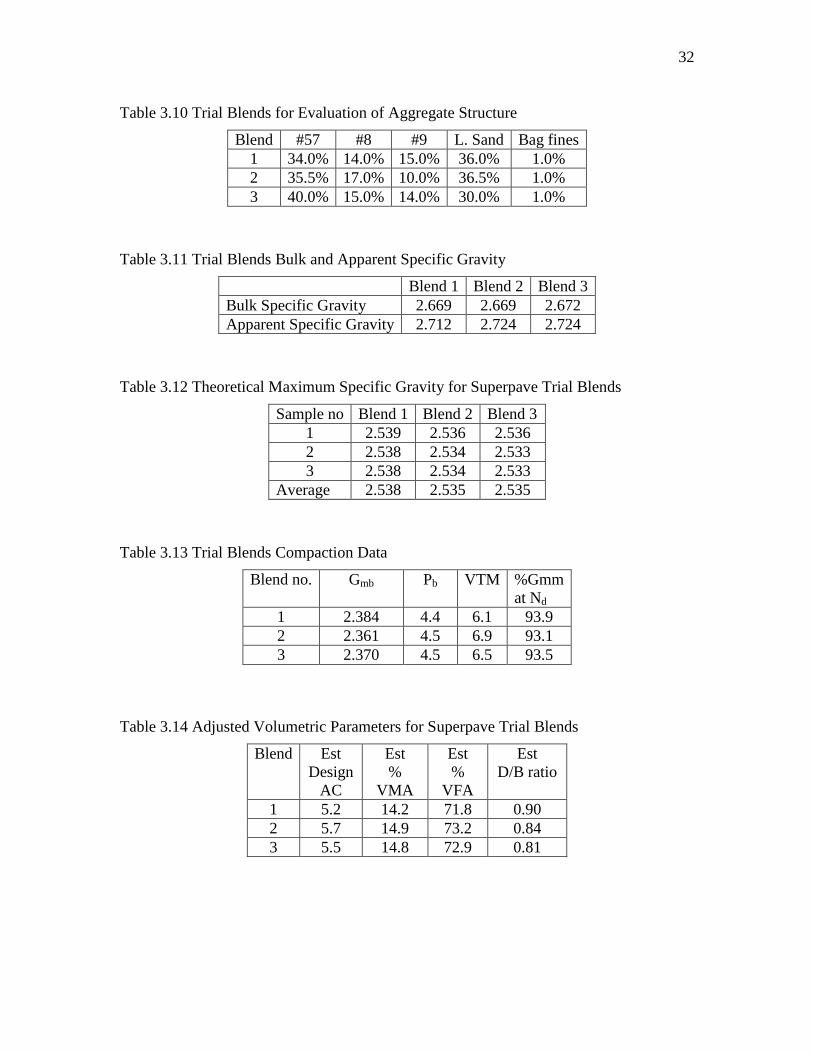
3.8.1 AGGREGATE TRIAL BLENDS
Three trial blends were evaluated to determine the best aggregate structure. The
percent of each aggregate type in the trial blends are shown in Table 3.10; the gradation
chart is shown in Figure 3.2. All the three trial blends were within the control points of
19mm nominal maximum size and below the restricted zone (Table 2.5). The restricted
zone is meant to be a guide to help ensure that too much natural sand is not used in the
mixture and to help ensure that minimum VMA requirements are met.
Page 39
30
The aggregate consensus property test values for aggregate blends and the
combined average aggregate bulk and apparent specific gravities were determined using
the Equation 2.8 and 2.2, respectively, and are presented in Table 3.11
The initial binder contents for heavy-traffic level mix design were computed
using the Equations 2.9 to 2.13. The initial binder content was 4.4% for blend 1 and 4.5%
for blend 2 and blend 3.
Three samples for each trial blend at their corresponding initial binder content
were tested to determine the average Theoretical Maximum Specific Gravity (AASHTO
T209) in Table 3.12.
3.8.2 DESIGN AGGREGATE STRUCTURE
Three samples for each trial blend at their corresponding initial binder content
were compacted to 100 gyrations, which is Nd for heavy traffic level. The bulk specific
gravity (AASHTO T 166) and volumetrics (Equations 2.3 to 2.5) of the compacted
samples were determined and the average values are presented in Table 3.13.
The estimated design asphalt content was computed using Equation 2.17. The
volumetric data at the estimated design asphalt content for all three blends were
computed (Equations 2.18 to 2.21) and summarized in Table 3.14.
All the three blends meet the Superpave volumetric criteria, Table 2.3. The trial
Blend 1 was selected as design aggregate structure for Heavy Traffic level Superpave
mix design because it was used by J.F. Allen Company for a Superpave project in West
Virginia and has proven performance.
The initial binder content of Superpave mix design for medium and light traffic
levels was estimated to be 5.0%. Three samples with blend 1 were tested to determine the
average Theoretical Maximum Specific Gravity (AASHTO T209) at 5.0% asphalt
content.
Page 40
31
FIGURE 3.2 Superpave trial blend gradations
0
10
20
30
40
50
60
70
80
90
100
Perc
en
t p
assin
g
Sieve size
0.075 1912.5 9.54.752.361.180.60.3 25
Page 41
32
Table 3.10 Trial Blends for Evaluation of Aggregate Structure
Blend #57 #8 #9 L. Sand Bag fines
1 34.0% 14.0% 15.0% 36.0% 1.0%
2 35.5% 17.0% 10.0% 36.5% 1.0%
3 40.0% 15.0% 14.0% 30.0% 1.0%
Table 3.11 Trial Blends Bulk and Apparent Specific Gravity
Blend 1 Blend 2 Blend 3
Bulk Specific Gravity 2.669 2.669 2.672
Apparent Specific Gravity 2.712 2.724 2.724
Table 3.12 Theoretical Maximum Specific Gravity for Superpave Trial Blends
Sample no Blend 1 Blend 2 Blend 3
1 2.539 2.536 2.536
2 2.538 2.534 2.533
3 2.538 2.534 2.533
Average 2.538 2.535 2.535
Table 3.13 Trial Blends Compaction Data
Blend no. Gmb Pb VTM %Gmm
at Nd
1 2.384 4.4 6.1 93.9
2 2.361 4.5 6.9 93.1
3 2.370 4.5 6.5 93.5
Table 3.14 Adjusted Volumetric Parameters for Superpave Trial Blends
Blend Est
Design
AC
Est
%
VMA
Est
%
VFA
Est
D/B ratio
1 5.2 14.2 71.8 0.90
2 5.7 14.9 73.2 0.84
3 5.5 14.8 72.9 0.81
Page 42
33
Samples at 5.0% asphalt content were compacted using 75 gyrations and 50
gyrations, which is the design number of gyrations for light and medium traffic level
respectively. Two samples were prepared at each compaction level. The volumetric
results determined using Equations 2.3 to 2.5 are shown in Table 3.15.
Table 3.15 Blend 1 Volumetric Parameters for Medium and Light Traffic Level Mix
Designs
Traffic level Avg. Gsb Avg. Gmm Pb VTM VMA %Gmm at Nd
Medium 2.367 2.513 5.0 5.8 15.8 94.2
Light 2.513 2.513 5.0 7.6 17.3 92.4
The estimated design asphalt content for medium and light traffic level Superpave
mixes was computed using Equation 2.17. The volumetric data at the estimated design
asphalt content for the two traffic levels are computed (Equations 2.18 to 2.21) and
presented in Table 3.16.
Table 3.16 Adjusted Volumetric Parameters for Medium and Light Traffic Level Mix
Designs
Traffic level Estimated
Design AC
Estimated
% VMA
Estimated
% VFA
Estimated
D/B
Medium 5.7 15.4 75.9 0.81
Light 6.4 16.6 74.0 0.71
The volumetric parameters at the estimated design asphalt content met Superpave
criteria and hence blend 1 was selected as design aggregate structure for the medium and
light traffic level Superpave mixes.
3.8.3 DESIGN ASPHALT CONTENT
The design aggregate structure process showed the same aggregate blends could
be used for all traffic levels. The estimated asphalt contents were 6.4%, 5.7%, and 5.2%
for the light, medium and heavy traffic levels respectively. The first procedure for
determining the design binder content is to measure Gmm. Since the binder content the
medium and heavy traffic were separated by 0.5%, six binder contents cover the needed
binder contents for Gmm testing; 4.7 to 6.7% at 0.5% increments. The Gmm for the low
Page 43
34
traffic level was determined for percent binder contents of 5.9 to 7.4% in 0.5%
increments. Table 3.17 gives the average Gmm values at each asphalt content.
Table 3.17 Average Gmm Values for Superpave Mixes
Asphalt Content
Percent
Average
Gmm
4.7% 2.523
5.2% 2.502
5.7% 2.495
6.2% 2.485
6.7% 2.464
5.9% 2.487
6.4% 2.469
6.9% 2.452
7.4% 2.434
Two samples each at 4.7%, 5.2%, 5.7%, and 6.2% asphalt content were
compacted to 100 gyrations. The average bulk specific gravities determined (AASHTO
T166) and the volumetrics computed using Equations 2.2 to 2.5 at each asphalt content
were tabulated in Table 3.18.
Table 3.18. Volumetric Data for Superpave Heavy Traffic Level.
Percent Asphalt Content Air voids % Gmm,Nd VMA at Nd VFA Nd Avg Gmb
4.7 5.3 94.7 14.7 63.8 2.389
5.2 3.8 96.2 14.5 73.6 2.406
5.7 3.0 97.0 14.6 79.3 2.420
6.2 2.7 97.3 15.0 82.3 2.419
Two samples each at 5.2%, 5.7%, 6.2%, and 6.7% asphalt content were
compacted to 75 gyrations. The average bulk specific gravities determined (AASHTO
T166) and the volumetrics computed using Equations 2.2 to 2.5 at each asphalt content
were tabulated in Table 3.19.
Page 44
35
Table 3.19 Volumetric Data for Superpave Medium Traffic Level
Percent Asphalt
Content
Air voids % Gmm,Nd VMA at Nd VFA Nd Avg Gmb
5.2 5.2 94.7 15.7 67.2 2.373
5.7 4.0 96.2 15.4 73.8 2.394
6.2 3.4 97.0 15.7 78.1 2.400
6.7 2.4 97.3 15.9 85.2 2.406
Two samples each at 5.9%, 6.4%, 6.9%, 7.4% asphalt content were compacted to
50 gyrations. The average bulk specific gravities determined (AASHTO T166) and the
volumetrics computed using Equations 2.2 to 2.5 at each asphalt content were tabulated
in Table 3.20.
Table 3.20 Volumetric Data for Superpave Light Traffic Level
Percent Asphalt Content Air voids % Gmm,Nd VMA at Nd VFA Nd Avg Gmb
5.9 4.8 95.2 16.5 71.0 2.368
6.4 3.7 96.3 16.6 77.6 2.377
6.9 2.8 97.2 16.8 83.5 2.384
7.4 1.6 98.4 16.9 90.7 2.396
The volumetric data was plotted versus asphalt content for all three traffic design
levels. The design asphalt content corresponding to 4.0% air voids was determined for
three mixes. The volumetric properties at design asphalt content were determined from
the plots. The summary of the three mix designs is shown in Table 3.21.
Table 3.21 Summary of Superpave Mix Designs.
Design Traffic Level Design
AC
% Gmm,Nd VTM VMA VFA
Heavy 5.1 96.0 4.0 14.5 70.2
Medium 5.7 96.0 4.0 15.4 73.7
Traffic 6.2 96.0 4.0 16.6 75.0
The complete data and interim calculations of Superpave mix designs are
presented in Appendix C.
Page 45
36
3.9 SPECIMENS FOR APA TESTING
The Superpave Gyratory Compactor was used to make the specimens for testing
with the APA. The APA specimens were made to 95 mm height with 7.0 0.5 % air
voids range. The specimens out of this air voids range were discarded.
3.10 ASPHALT PAVEMENT ANALYZER RUNS
The APA procedure described in Chapter 2 was followed to obtain rut depth
results of the specimens. All samples were tested at 140oF with a hose pressure of 100 psi
and a wheel load of 100 lb. Rut depths were measured after 8000 cycles.
There are 18 combinations of factors and levels. The combinations of mix design
and traffic levels were assigned a treatment number as defined in Table 3.19. Two sets of
test results were obtained for each combination, providing 36 experimental units. Each
test result is an average of two test specimens, one in the front position of the mould and
the other in the back. The factor levels in the experimental design were:
Factors Levels
Mix design method Superpave, Marshall
Traffic level Light, Medium, High
APA position Left, Center, Right
Table 3.19 Treatments Used in Experimental Design
Treatment
No.
Type of mix
design
Design
traffic level
1 Superpave Heavy
2 Superpave Medium
3 Superpave Light
4 Marshall Heavy
5 Marshall Medium
6 Marshall Light
The WVDOH uses the medium traffic level for all pavements with less than 3
million ESALs. Thus, the Marshall medium traffic level mix design was used to prepare
the samples for the Marshall light traffic level. Since the Marshall light and medium
traffic level mix designs were equivalent one would expect similar performance.
Page 46
37
To minimize the effects of position in the APA machine and test sequence, the
order of testing the specimens was randomized. The Table 3.20 presents the order of
testing the specimens and average rut depth results.
Table 3.20 Rut Depth Results.
Positions
Left Center Right
APA TEST
SEQUENCE
1 2 3
1 5.591* 6.16 2 9.39 3
2 9.34 6 4.73 1 9.32 5
3 6.26 5 5.80 4 4.75 6
4 9.39 3 9.17 5 6.45 3
5 8.39 2 4.61 6 5.03 4
6 5.26 3 3.89 4 6.90 1
7 4.09 1 6.54 2 6.58 6
8 6.32 4 6.53 3 6.02 2
9 9.29 6 5.09 5 5.62 4
10 6.83 2 3.62 1 7.68 5
11 5.20 4 5.49 3 6.58 2
12 8.70 5 8.50 6 5.12 1
*Subscript indicates treatment number as defined
in Table 3.19
3.11 TESTS FOR OTHER CRITERIA
Two samples for each mix design were evaluated to check for the other mix
design criteria. Marshall samples were made using Superpave mix designs and checked
for the criteria and vice versa. Both the mix designs passed the other mix design’s
criteria. The data are presented in Appendix D.
Page 47
38
CHAPTER 4 RESULT AND ANALYSIS
There are indications in the literature that Superpave mixes have lower optimum
binder content than Marshall mixes. This was not the case for the mixes designed during
the research. The Superpave mixes consistently had a greater binder content than
Marshall mixes, ranging from 0.2% to 0.7% higher. The largest range was for the
Superpave light traffic level versus the Marshall, since the WVDOH does not have
Marshall procedure for light traffic level, the Superpave light traffic design was
compared to a Marshall medium traffic design.
An Analysis of Variance shown in Figure 4.1 was performed using the SAS
program. The factors of mix design type, test sequence, and position indicate that there is
insufficient evidence to identify a difference. The traffic level indicates a difference at the
95% confidence level. The interaction effect of mix design type versus traffic level
indicates there is not sufficient evidence to identify a difference.
The confidence interval for the difference in the means of two mixes is –1.98 to
0.62. This interval is not within the detection limits.
The SAS program was run to compare possible combinations of mix and traffic
on one to one bases. The results were used to compute a confidence interval about the
difference in the adjusted means as:
21,
2
'
2
'
1 SEt df (Eqn. 4.1)
where,
’1=adjusted mean 1
’2=adjusted mean 2
SE=standard error
If the test is conducted a number of times under the same conditions, the
difference in the adjusted means would fall within this range, 95% of the time.
Page 48
39
Fig 4.1 Output of Analysis of Variance _________________________________________________________________________________________
The GLM Procedure
Class Level Information
Class Levels Values
mix 2 1 2
traf 3 1 2 3
seq 12 1 2 3 4 5 6 7 8 9 10 11 12
posit 3 1 2 3
Number of observations 36
The GLM Procedure
Dependent Variable: depth
Sum of
Source DF Squares Mean Square F Value Pr > F
Model 18 67.1728747 3.7318264 1.67 0.1491
Error 17 38.0637559 2.2390445
Corrected Total 35 105.2366306
R-Square Coeff Var Root MSE rutd Mean
0.638303 22.99807 1.496344 6.506389
Source DF Type I SS Mean Square F Value Pr > F
mix 1 1.80902500 1.80902500 0.81 0.3813
traf 2 32.72620556 16.36310278 7.31 0.0051
mix*traf 2 1.19761667 0.59880833 0.27 0.7685
seq 11 22.41098858 2.03736260 0.91 0.5514
position 2 9.02903889 4.51451944 2.02 0.1638
Source DF Type III SS Mean Square F Value Pr > F
mix 1 2.73985482 2.73985482 1.22 0.2841
traf 2 23.79695449 11.89847725 5.31 0.0161
mix*traf 2 0.92319986 0.46159993 0.21 0.8157
seq 11 22.41098858 2.03736260 0.91 0.5514
position 2 9.02903889 4.51451944 2.02 0.1638
The GLM Procedure
Level of -----depth----------
Mix N Mean Std Dev
1 18 6.28222222 1.58252425
2 18 6.73055556 1.89198145
Level of -------depth-----------
traf N Mean Std Dev
1 12 5.15916667 0.97764521
2 12 7.22833333 1.38264459
3 12 7.13166667 1.92986026
Level of Level of ---------depth--------
Mix traf N Mean Std Dev
1 1 6 5.00833333 1.16425799
1 2 6 6.75333333 0.85439257
1 3 6 7.08500000 1.85536789
2 1 6 5.31000000 0.83224996
2 2 6 7.70333333 1.71297013
2 3 6 7.17833333 2.17852626
The GLM Procedure
Dependent Variable: depth
Parameter Estimate Error t Value Pr>|t|
Mix -0.68245326 0.61693654 -1.11 0.2841
_________________________________________________________________________________________
Page 49
40
Table 4.1 shows the range of the difference in adjusted means computed from the
results of the SAS General Linear Models procedure. When zero is outside the range,
there is an indication of consistent difference in the test result. The comparisons which
doesn’t include zero in its range are
Superpave Light – Superpave Heavy
Superpave Medium - Superpave Heavy
Marshall Medium - Marshall Heavy
Marshall Light - Marshall Heavy
These comparisons are consistent with the concept, mixes for higher traffic levels
are designed for higher rut resistance.
Zero within the range for the comparisons of the different mix design methods for
a given traffic level is consistent with the ANOVA result.
Table 4.1 Confidence Interval Computed for Various Parameters
Comparison SAS program Results Confidence interval range
1 2 Estimate Standard Error Lower limit Upper limit
SPL ML 0.515 1.120 -2.88 1.85
SPL MM 0.641 1.052 -2.86 1.58
SPL MH -0.803 0.996 -1.75 2.43
SPM ML 0.176 1.005 -2.29 1.94
SPM MM 0.302 1.026 -2.47 1.86
SPM MH -1.142 0.953 -0.87 3.15
SPH ML 2.549 0.958 -4.57 -0.53
SPH MM 2.675 0.953 -4.69 -0.66
SPH MH 1.231 1.020 -3.38 0.92
SPL SPM 0.339 0.990 -1.75 2.43
SPL SPH -2.034 1.041 2.60 6.67
SPM SPH 2.034 1.040 -4.23 -0.16
ML MM 0.126 0.923 -2.073 1.821
ML MH -1.318 0.971 0.73 3.37
MM MH -1.444 0.993 0.65 3.54
Page 50
41
CHAPTER 5 CONCLUSIONS AND RECOMMENDATIONS
5.1 CONCLUSIONS
Based on the laboratory effort and statistical analysis of data, the following
conclusions were made:
The statistical analysis does not provide enough evidence to say that there is a
difference in the Superpave and Marshall mix design methodologies.
The ANOVA indicated a difference due to traffic levels. The multiple
comparison procedure indicated that mixes designed for higher traffic levels
are more rut resistant than mixes designed for lower traffic levels.
The mixes prepared under the Superpave method passed the Marshall criteria.
The mixes prepared under the Marshall method passed the Superpave criteria.
This indicates that contractors using Marshall methodology to design and
construct pavements should not face unusual difficulties with Superpave
mixes.
The asphalt contents of Superpave mix designs are higher than Marshall mix
design for the same traffic level.
5.2 RECOMMENDATIONS
Based on the information developed during this research, differences between
the Marshall Base II and Superpave 19 mm mixes, evaluated for all traffic
levels, could not be detected statistically. Thus, it would appear that
Superpave implementation could proceed with concerns about pavement
performance.
The fact that the Superpave mixes required slightly higher asphalt content
would increase the cost of the mixes. For non-NHS roads, this may be
beneficial as pavement performance, other than rutting, is generally improved
with the higher asphalt film thickness associated with higher asphalt contents.
Page 51
42
5.3 FUTURE RESEARCH
Similar analysis could be done using PG 64-22, which is generally used for
non-NHS roads in WV.
More aggregate types should be studied to have a broader perspective. This
study was limited to one source of limestone aggregates. Other aggregates
commonly used in the state should be studied, including other limestone
sources and natural sands.
Field tests on the rutting performance should be considered. The performance
evaluation performed during this study is based on rutting potential as
evaluated by the APA. An alternative method for estimating the performance
of low volume mixes is needed, since rutting may not be the controlling
performance parameter on low volume roads.
Page 52
43
REFERENCES
1. Huber G.A., Jones J. Chris, Messersmith E. Paul, Jackson N. Mike. Contribution
of Fine Aggregate Angularity and Particle Shape to Superpave Mixture
Performance. Transportation Research Record 1609. 1997.
2. Kandhal P.S, Mallick B.R. Evaluation of Asphalt Pavement Analyzer for HMA
Design. National Center for Asphalt Technology. April 1999.
3. Mallick B. Rajib, Buchanan Shane, Brown E.R, Huner Mike. An Evaluation of
Superpave Gyratory Compaction of Hot Mix Asphalt. National Center for Asphalt
Technology. May 1998.
4. Roberts L. Freddy, Kandhal S. Prithvi, Brown E. Ray, Lee Dah-Yim, Kennedy W.
Thomas. Hot Mix Asphalt Materials, Mixture Design and Construction. NAPA
Education Foundation, MD.1996.
5. Harman Thomas, D’Angelo John, Bukowski John. Superpave Asphalt Mixture
Design-Workshop. Federal Highway Administration. 1999.
6. Cooley L.A. Jr., Kandhal P.S, Buchanan M.S, Fee F, Epps A. Loaded Wheel
Testers in the United States: State of Practice. National Center for Asphalt
Technology. April 2000.
7. Background of Superpave Asphalt Mixture Design and Analysis. Federal Highway
Administration. Report number FHWA-SA-95-003, 1995.
8. Implementation Survey IV, 1999-2000. Federal Highway Administration. July
2000
[http://ce.ecn.purdue.edu/~spave/Technical%20Info/Meetings/Imp99-00.htm]
9. Ruggedness Evaluation of AASHTO TP4, The Superpave Gyratory Compactor.
The Superpave Asphalt research Program, The University of Texas, Austin. 1996.
[http://www.utexas.edu/research/articles/sgcrugg.html]
Page 53
44
10. Huber A. Gerald. Development of the Superpave Gyratory Compactor. The
Superpave Asphalt Research Program, The University of Texas, Austin. 1996.
[http://www.utexas.edu/research/superpave/articles/gyr-hist.html]
11. West C Randy. A Ruggedness Study of the Asphalt Pavement Analyzer Rutting.
APAC Materials Service. May 1999.
12. Cooley L. Allen Jr., Kandhal S. Prithvi. Evaluation of Density Gradients in APA
Samples. National Center for Asphalt Technology. October 1999.
SPECIFICATIONS
1. WVDOH Standard Specifications, 2000.
2. Guide to Designing Hot-Mix Asphalt using the Marshall Design Method.
WVDOT MP 401.02.22. 2000
3. Guide to designing Hot-Mix Asphalt using the Superpave Volumetric Design
System. WVDOT MP 401.02.28. 2000
4. Bulk Specific Gravity of Bituminous Mixtures. AASHTO T166. 1993.
5. Maximum Specific Gravity of Bituminous Paving Mixtures. AASHTO T209.
1994.
6. Resistance to Plastic Flow of Bituminous Mixtures Using Marshall Apparatus.
AASHTO T245. 1993.
7. Method for Preparing and Determining the Density of HMA specimens by Means
of the Superpave Gyratory Compactor. AASHTO TP4. 2000
8. Determining the Percentage of Fractured Particles in Coarse Aggregate. ASTM
D 5821.
9. Flat or Elongated Particles in Coarse Aggregate. ASTM D 4791.
10. Plastic Fines in Graded Aggregates and Soils by Use of the Sand Equivalent Test.
AASHTO T 176.1986
11. Uncompacted Void Content of Fine Aggregate. AASHTO T304. 1998.
Page 54
45
12. Determination of Specific Gravity and Absorption of Coarse Aggregate.
AASHTO T85. 1991.
13. Determination of Specific Gravity and Absorption of Fine Aggregate. AASHTO
T84. 1994.
14. Amount of Material Passing #200 Sieve. ASTM C117. 1984.
15. Sieve Analysis. ASTM C136. 1984.
Page 55
46
APPENDIX A AGGREGATE TESTS AND PROPERTIES
Table A.1 Gradation Data for Aggregates
#8 Coarse Aggregate
Sample Sample1 Sample 2 Sample 3
SIEVE Wt % Wt. % Wt % Wt. % Wt % Wt. %
SIZE, mm retained retained Passing retained Retained Passing retained retained Passing
25 0 0 100 0 0 100 0 0 100
19 0 0 100 0 0 100 0 0 100
12.5 0 0 100 0 0 100 0 0 100
9.5 37 3.7 96 40.5 3.8 96 56.4 4.9 95
4.75 836 83 13 836.2 78.6 18 965.9 83.9 11
2.36 108 11 2.6 131 12 5.3 98 8.5 2.6
1.18 7.6 0.8 1.9 23 2.2 3.1 8 0.7 1.9
0.6 1.7 0.2 1.7 8.2 0.8 2.3 1.8 0.2 1.8
0.3 0.8 0.1 1.6 4.1 0.4 2.0 1.1 0.1 1.7
0.075 1.3 0.1 1.5 4.3 0.4 1.6 1.6 0.1 1.5
Pan 14.9 1.5 16.5 1.6 17.5 1.5
Total 1007 1063.9 1150.7
#9 Coarse Aggregate
Sample Sample1 Sample 2 Sample 3
SIEVE Wt % Wt. % Wt % Wt. % Wt % Wt. %
SIZE,
mm retained retained Passing retained retained Passing retained retained Passing
25 0 0 100 0 0 100 0 0 100
19 0 0 100 0 0 100 0 0 100
12.5 0 0 100 0 0 100 0 0 100
9.5 0 0 100 0 0 100 0 0 100
4.75 175 32 68 183.2 32.3 68 157.8 28.6 71
2.36 346 64 4.1 359 63 4.5 360 65 6.3
1.18 13 2.3 1.8 14 2.5 2.0 21 4 2.5
0.6 0.4 0.1 1.7 1.2 0.2 1.8 2.4 0 2.0
0.3 0.1 0.0 1.7 0.2 0.0 1.8 0.7 0 1.9
0.075 0.2 0.0 1.7 0.7 0.1 1.7 1.4 0 1.7
Pan 9.1 1.7 9.4 1.7 9.2 1.7
Total 543.6 567.4 552
Page 56
47
Table A.1 Gradation Data for Aggregates (continued)
SAND
Sample Sample1 Sample 2 Sample 3
SIEVE Wt % Wt. % Wt % Wt. % Wt % Wt. %
SIZE,
mm retained retained Passing retained retained Passing retained retained Passing
25 0 0 100 0 0 100 0 0 100
19 0 0 100 0 0 100 0 0 100
12.5 0 0 100 0 0 100 0 0 100
9.5 0 0 100 0 0 100 0 0 100
4.75 5.6 1.1 99 5.9 1.1 99 4.4 0.8 99
2.36 111 21 78 117 22 77 119 23 76
1.18 166 31 46 168 32 45 165 31 45
0.6 91 17 29 88 17 28 87 17 28
0.3 62 12 18 58 11 17 59 11 17
0.075 58 11 6.6 54 10 6.5 55 10 6.6
Pan 35 6.6 34 6.5 35 6.6
Total 528.8 525.4 522.8
Table A.2 Specific Gravity of Aggregates
#57 #8
Sample No. Sample No.
1 2 3 1 2 3
Dry Wt. (g), A 4886.3 3790.6 3789.8 2756.1 1746.7 1741.3
SSD Wt.(g), B 4918.2 3812.6 3811.3 2773.8 1758.2 1752.6
Wet Wt. (g), C 3098.8 2403.1 2400.6 1752.4 1106.4 1102.9
Bulk SG 2.686 2.689 2.686 2.698 2.680 2.680
A/(B-C)
Apparent SG 2.734 2.732 2.728 2.746 2.728 2.728
A/(A-C)
Absorption, % 0.7 0.6 0.6 0.6 0.7 0.6
Page 57
48
Table A.2 Specific Gravity of Aggregates (continued)
#9 Sand
Sample No.
1 2 3 1 2 3
Dry Wt. (g), A 495.7 495.4 496.6 493.1 493.6 493.4
Pycnometer Wt.(g),
B 1448.2 1448.2 1448.2 1448.2 1448.2 1448.2
Wt. In water (g), C 1761.8 1762.5 1763.2 1761.9 1762.5 1762.3
SSD Wt.(g), D 500.3 500 501.1 500 500.6 500.5
Bulk SG 2.655 2.668 2.673 2.647 2.649 2.647
A/(B+D-C)
Apparent SG 2.722 2.736 2.739 2.749 2.753 2.752
A/(B+A-C)
Absorption,% 0.9 0.9 0.9 1.4 1.4 1.4
Table A.3. Aggregate Consensus Property Tests
Sand
Sample Sand Clay Equivalency
No.
reading
(A)
reading
(B) (A-10)/B*100
1 13.4 4.3 79
2 13.5 4.5 78
3 13.5 4.5 78
Aggregate
type
mass of fine
aggregate
(g)
Fine
aggregate
angularity
Sand 146.0 45.9
# 9 146.4 46.0
# 8 146.9 45.6
Page 58
49
APPENDIX B MARSHALL MIX DESIGN DATA AND ANALYSIS
Table B.1 Theoretical Maximum Specific Gravity Calculations
AC Sample Dry Wet Container Gmm
Wt. (g) Wt. (g) Wt. (g)
3.9 1 2071.1 2769.2 1511.1 2.547
2 2067.5 2766.9 1511.1 2.547
3 2072.9 2771 1511.1 2.550
4.4 1 2073.1 2766.2 1511.1 2.534
2 2072.8 2765.8 1511.1 2.534
3 2075.3 2767.6 1511.1 2.535
4.9 1 2086.2 2767 1511.1 2.513
2 2086.7 2769.9 1511.1 2.520
3 2029.2 2733.5 1511.1 2.515
5.4 1 2095.5 2583.9 1511.1 2.049
2 2093.2 2579.2 1511.1 2.042
3 2097 2583.2 1511.1 2.046
5.9 1 2110.6 2588.2 1511.1 2.042
2 2110.9 2587.7 1511.1 2.041
3 2109.2 2587 1511.1 2.041
6.4 1 2111.3 2583.8 1511.1 2.033
2 2110 2582.3 1511.1 2.031
3 2114.4 2586.3 1511.1 2.035
6.9 1 2106.9 2576.6 1511.1 2.023
2 2105.6 2575.2 1511.1 2.022
3 2107.5 2577.3 1511.1 2.024
7.4 1 2092.5 2562.6 1511.1 2.010
2 2098.6 2565 1511.1 2.009
3 2102.4 2568 1511.1 2.011
Page 59
50
Table B.2 Marshall Heavy Traffic Level Mix Design
Asphalt Content by Mass in Grams Specific Gravity Voids in Percent Air Voids Stability (n) Flow
Weight of Mix Specimen Weight Weight Saturated Density Mineral Pounds 0.01
Specimen Percent Thickness in Air In water surface dry Bulk Maximum Kg/m3 Aggregate Total Mix Filled Actual Adjusted inch
Number AC (mm) A C B D E F
100 X 100 X
A/(B-C) D X 1000 [(E-D)/E] [(F-G)/F]
1 3.9 66 1187.9 686.5 1194.2 2.340 2425 2287.1 16.0
2 3.9 65 1186.6 688.3 1193.2 2.350 2350 2261.9 14.0
3 3.9 65 1185.6 687.8 1192.3 2.350 2225 2141.6 13.5
Average 2.347 2.55 2347 15.54 7.97 48.68 2333 2230.2 14.5
1 4.4 66 1184.3 692.5 1190.1 2.380 2000 1886.3 17.5
2 4.4 64 1184.6 694.8 1190.4 2.390 2350 2320.6 17.5
3 4.4 66 1181.2 695.1 1187.2 2.400 2475 2334.2 16.0
Average 2.390 2.533 2390 14.42 5.64 60.90 2275 2180.4 17.0
1 4.9 63 1187.2 694.8 1190.3 2.396 2025 2050.3 12.5
2 4.9 63 1174.5 689.5 1178.8 2.400 2125 2151.6 12.5
3 4.9 64 1190.4 701.5 1195.4 2.410 1875 1851.6 13.0
Average 2.402 2.513 2402 14.44 4.41 69.46 2008 2017.8 12.7
1 5.4 64 1182 696 1186.4 2.410 1975 1950.3 13.5
2 5.4 63 1180.7 690.7 1184.7 2.390 2000 2025.0 13.0
3 5.4 66 1179.4 688.1 1183.5 2.381 2175 2051.3 22.5
Average 2.394 2.491 2394 15.19 3.91 74.28 2050 2008.9 16.3
1 5.9 63 1188.9 695.3 1191.1 2.398 2450 2480.6 15.0
2 5.9 63 1185.3 693.2 1189.3 2.389 2300 2328.8 15.0
3 5.9 64 1184.5 692.6 1188.2 2.390 2275 2145.6 16.0
Average 2.392 2.476 2392 15.68 3.38 78.47 2342 2318.3 15.3
Page 60
51
Table B.3 Marshall Medium Traffic Mix Design
Asphalt Content by Mass in Grams Specific Gravity Voids in Percent Air Voids Stability (n) Flow
Weight of Mix Specimen Weight Saturated Weight in Density Mineral Pounds 0.01
Specimen Percent Thickness in Air surface dry water Bulk Maximum Kg/m3 Aggregate Total Mix Filled Actual Adjusted inch
Number AC (mm) A B C D E F G
100 X 100 X
A/(B-C) D X 1000 [(E-D)/E] [(F-G)/F]
1 4.4 62 1136.7 1142.3 658.0 2.347 1950 2023 14
2 4.4 61 1140.7 1144.6 662.3 2.365 1975 2110 15
3 4.4 61 1138.1 1142.5 661.0 2.364 2025 2163 15
Average 2.359 2.534 2359 15.55 6.92 55.49 1983 2099 15
1 4.9 61 1145.7 1150.1 665.0 2.362 2025 2163 16
2 4.9 61 1141.9 1147.7 663.9 2.36 2050 2190 17
3 4.9 61 1141.5 1146.9 663.8 2.363 2050 2190 17
Average 2.362 2.516 2362 15.88 6.14 61.37 2042 2163 17
1 5.4 61 1139.5 1142.9 663.2 2.375 2000 2136 19
2 5.4 62 1140.9 1144.5 665.2 2.380 2000 2075 18
3 5.4 61 1139.2 1144.0 664.4 2.375 1850 1976 20
Average 2.377 2.491 2377.000 15.78 4.58 71.01 1950 2163 19
1 5.9 61 1143.8 1146.6 667.2 2.386 1950 2083 15
2 5.9 60 1138.0 1140.3 664.4 2.391 1975 2134 15
3 5.9 61 1144.6 1146.8 671.5 2.408 1875 2003 13
Average 2.395 2.476 2395 15.59 3.27 79.04 1933 2073 14.3
1 6.4 60 1137.6 1139.4 669.0 2.418 1825 1972 21
2 6.4 61 1138.5 1141.5 662.5 2.377 1975 2110 20
3 6.4 61 1150.9 1154.2 673.1 2.392 1925 2056 20
Average 2.396 2.452 2396 16.01 2.29 85.69 1908 2046 20
Page 61
52
2340
2350
2360
2370
2380
2390
2400
2410
3 3.5 4 4.5 5 5.5 6 6.5
Asphalt content, %
De
nsit
y, k
g/m
3
Figure B.1 Asphalt content versus Density – Marshall heavy
1950
2000
2050
2100
2150
2200
2250
2300
2350
3 3.5 4 4.5 5 5.5 6 6.5
Asphalt content, %
Sta
bilit
y, p
ou
nd
s
Figure B.2 Asphalt content versus Stability – Marshall heavy traffic mix.
Page 62
53
Figure B.3 Asphalt content versus Flow – Marshall heavy traffic mix
Figure B.4 Asphalt content versus VTM – Marshall heavy traffic mix
12
13
14
15
16
17
18
3 3.5 4 4.5 5 5.5 6 6.5
Asphalt content, %
Flo
w
3
4
5
6
7
8
9
3 3.5 4 4.5 5 5.5 6 6.5
Asphalt content, %
VT
M, %
Page 63
54
Figure B.5 Asphalt content versus VMA – Marshall heavy traffic mix
Figure B.6 Asphalt content versus VFA –Marshall heavy traffic mix.
14.2
14.4
14.6
14.8
15
15.2
15.4
15.6
15.8
16
3 3.5 4 4.5 5 5.5 6 6.5
Asphalt content, %
VM
A, %
30
40
50
60
70
80
90
3 4 5 6 7
Asphalt content, %
VF
A,
%
Page 64
55
Figure B. 7 Asphalt content versus density, Marshall medium traffic mix.
Figure B.8 Asphalt content versus Stability – Marshall medium traffic mix.
2355
2360
2365
2370
2375
2380
2385
2390
2395
2400
4 4.5 5 5.5 6 6.5 7
Asphalt content, %
Den
sit
y,
Kg/m
3
2040
2060
2080
2100
2120
2140
2160
2180
4 4.5 5 5.5 6 6.5 7
Asphalt content, %
Sta
bility
, p
oun
ds
Page 65
56
0.0
5.0
10.0
15.0
20.0
25.0
4 4.5 5 5.5 6 6.5 7
Asphalt content, %
Flo
w, 0.0
1 in
ch
Figure B.9 Asphalt content versus Flow – Marshall light traffic level
2.0
3.0
4.0
5.0
6.0
7.0
8.0
4 4.5 5 5.5 6 6.5 7
Asphalt content, %
Air
vo
ids
, %
Figure B.10 Asphalt content versus Air voids –Marshall medium traffic mix.
Page 66
57
15.5
15.6
15.7
15.8
15.9
16.0
16.1
4 4.5 5 5.5 6 6.5 7
Asphalt content, %
VM
A, %
Figure B.11 Asphalt content versus VMA – Marshall light traffic mix.
55.0
60.0
65.0
70.0
75.0
80.0
85.0
90.0
4 4.5 5 5.5 6 6.5 7
Asphalt content, %
VF
A, %
Figure B.12 Asphalt content versus VFA – Marshall
Page 67
58
APPENDIX C SUPERPAVE MIX DESIGN DATA AND ANALYSIS
Table C.1 Theoretical Specific Gravity for Trial Blends
Weight of the container in water, (g)[D] = 1511.1
A E A/(A+D-E)
BLEND AC,% Sample Dry wt.(g) Wet wt.(g) Gmm
1 4.4 1 2231.8 2864.0 2.539
2 2074.4 2768.2 2.538
3 2077.2 2769.8 2.538
2 4.5 1 2081.5 2771.8 2.536
2 2074.4 2766.9 2.534
3 2077.5 2768.8 2.534
3 4.5 1 2097.7 2770.6 2.503
2 2072.4 2771.5 2.552
3 2081.9 2771.1 2.533
Table C.2 Bulk Specific Gravity for Trial Blends
A B C A/(C-B)
Blend Sample Dry Wt. (g) Wet Wt. (g) SSD Wt. (g) Gmb
Blend 1 1 4767.6 2784.4 4788.1 2.379
2 4770.7 2791.2 4787.9 2.389
3 4778.2 2798.1 4803.3 2.383
Blend 2 1 4794.6 2795.0 4818.6 2.369
2 4786.0 2786.0 4814.0 2.360
3 4783.0 2781.0 4809.1 2.358
Blend 3 1 4941.4 2892.9 4968.4 2.381
2 4781.4 2787.2 4805.0 2.370
3 4767.5 2779.5 4798.5 2.361
Page 68
59
Table C.3 Theoretical Maximum Specific Gravity Calculations for Superpave Heavy
Traffic Mix
Weight of the container in water, (g) [D] = 1511.1
A E A/(A+D-E)
AC,% Sample Dry wt. (g) Wet wt. (g) Gmm Avg Gmm
4.7 1 2110.4 2785.2 2.523
2 2009.6 2723.9 2.522 2.523
5.2 1 2021.6 2724.7 2.502
2 2022.4 2725.2 2.502 2.502
5.7 1 2098.5 2768.2 2.494
2 2095.6 2767.1 2.496 2.495
6.2 1 2090.8 2760.2 2.484
2 2099.2 2765.9 2.486 2.485
Table C.4 Bulk Specific Gravity for Superpave Heavy Traffic Level Mix
Sample A B C A/(C-B)
AC, % No. Dry wt. (g) Wet wt. (g) SSD Wt. (g) Gmb Avg Gmb
4.7 1 4774.8 2787.1 4791.2 2.383
2 4759.6 2788.6 4776.2 2.395 2.389
6.4 1 4801.0 2808.3 4810.1 2.398
2 4765.0 2796.7 4771.5 2.413 2.406
6.9 1 4800.9 2825.2 4806.6 2.423
2 4775.2 2804.9 4781.2 2.416 2.420
7.4 1 4760.9 2802.1 4766.5 2.424
2 4755.2 2791.0 4762.0 2.413 2.419
Page 69
60
Figure C.1 Asphalt content versus Air voids-Superpave heavy traffic mix.
14.4
14.5
14.6
14.7
14.8
14.9
15.0
15.1
4.5 4.7 4.9 5.1 5.3 5.5 5.7 5.9 6.1 6.3
Asphalt content, %
VM
A, %
Figure C.2 Asphalt content versus VMA-Superpave heavy traffic mix.
2.0
2.5
3.0
3.5
4.0
4.5
5.0
5.5
4.5 4.7 4.9 5.1 5.3 5.5 5.7 5.9 6.1 6.3
Asphalt content, %
Air
vo
ids, %
Page 70
61
94.5
95.0
95.5
96.0
96.5
97.0
97.5
4.5 4.7 4.9 5.1 5.3 5.5 5.7 5.9 6.1 6.3
Asphalt content, %
Pe
rce
nt
Gm
m a
t N
d
Figure C.3 Asphalt content versus Percent Gmm at Nd-Superpave heavy traffic mix
60.0
65.0
70.0
75.0
80.0
85.0
4.5 5.0 5.5 6.0 6.5
Asphalt content, %
VF
A, %
Figure C.4 Asphalt content versus VFA – Superpave heavy traffic mix.
Page 71
62
Table C.5 Blend Bulk Specific Gravity Calculations –Superpave Medium Traffic Mix.
Sample A B C A/(C-B)
No. Dry Wt. (g) Wet Wt. (g) SSD Wt. (g) Gmb
1 4745.0 2742.5 4748.8 2.365
2 4753.2 2750.5 4768.8 2.355
3 4739.0 2762.9 4752.9 2.381
Table C.6 Theoretical Maximum Specific Gravity Calculations-Superpave Medium
Traffic Mix
Weight of the container in water, (g) [D] = 1511.1
A E A/(A+D-E)
AC,% Sample Dry wt. (g) Wet wt. (g) Gmm Avg Gmm
5.2 1 2013.4 2719.1 2.500
2 2021.6 2725.4 2.504 2.502
5.7 1 2092.8 2764.8 2.494
2 2098.5 2768.9 2.496 2.495
6.2 1 2088.4 2758.4 2.483
2 2090.8 2761.2 2.487 2.485
6.7 1 2099.4 2759.6 2.467
2 2110.9 2763.9 2.460 2.464
Table C.7 Bulk Specific Gravity-Superpave Medium Traffic Mix.
Sample A B C A/(C-B)
AC, % No. Dry wt. (g) Wet wt. (g) SSD Wt. (g) Gmb Avg Gmb
5.2 1 4730.4 2749.6 4743.3 2.373
2 4716.2 2740.8 4729.3 2.372 2.372
5.7 1 4760.1 2773.7 4769.7 2.385
2 4747.1 2779.2 4754.8 2.403 2.394
6.2 1 4652.2 2736.9 4657.9 2.422
2 4707.0 2765.6 4713.0 2.417 2.419
6.7 1 4734.2 2770.0 4742.4 2.400
2 4751.4 2787.5 4757.0 2.412 2.406
Page 72
63
2.0
2.5
3.0
3.5
4.0
4.5
5.0
5.5
5.0 5.2 5.4 5.6 5.8 6.0 6.2 6.4 6.6 6.8
Asphalt content, %
Air
vo
ids
, %
Figure C.5 Asphalt content versus Air voids-Superpave medium traffic mix.
14.8
15.0
15.2
15.4
15.6
15.8
16.0
5.0 5.2 5.4 5.6 5.8 6.0 6.2 6.4 6.6 6.8
Asphalt content, %
VM
A, %
Figure C.6 Asphalt content versus VMA-Superpave medium traffic level
Page 73
64
94.5
95.0
95.5
96.0
96.5
97.0
97.5
98.0
5.0 5.2 5.4 5.6 5.8 6.0 6.2 6.4 6.6 6.8
Asphalt content, %
Pe
rce
nt
of
Gm
m a
t N
d
Figure C.7 Asphalt content versus Percent of Gmm at Nd-Superpave medium traffic mix
60.0
65.0
70.0
75.0
80.0
85.0
90.0
5 5.2 5.4 5.6 5.8 6 6.2 6.4 6.6 6.8
Asphalt content,%
VF
A, %
Figure C.8 Asphalt content versus VFA-Superpave medium traffic mix.
Page 74
65
Table C.8 Blend Bulk Specific Gravity Calculations –Superpave Light Traffic Mix.
Sample A B C A/(C-B)
No. Dry Wt. (g) Wet Wt. (g) SSD Wt. (g) Gmb
1 4698.6 2704.4 4720.5 2.331
2 4684.5 2690.7 4711.9 2.318
3 4685.8 2701.1 4721.3 2.319
Table C.9 Theoretical Maximum Specific Gravity Calculations-Superpave Light Traffic
Mix.
Weight of the container in water, (g) [D] = 1511.1
A E A/(A+D-E)
AC,% Sample Dry wt. (g) Wet wt. (g) Gmm Avg Gmm
5.9 1 2061.3 2744 2.488
2 2072.4 2749.7 2.485 2.487
6.4 1 2148.0 2788.8 2.468
2 2144.3 2787.3 2.470 2.469
6.9 1 2103.6 2756.4 2.451
2 2100.2 2754.8 2.452 2.451
7.4 1 2124.9 2762.6 2.433
2 2110.4 2754.8 2.435 2.434
Table C.10 Bulk Specific Gravity-Superpave Light Traffic Mix.
Sample A B C A/(C-B)
AC, % No. Dry wt. (g) Wet wt. (g) SSD Wt. (g) Gmb Avg Gmb
5.9 1 4675.3 2710.7 4685.7 2.367
2 4638.8 2692.2 4651.5 2.368 2.367
6.4 1 4676.5 2721.0 4685.1 2.381
2 4653.2 2700.4 4662.3 2.372 2.376
6.9 1 4614.5 2682.7 4622.4 2.379
2 4645.9 2706.6 4651.3 2.389 2.384
7.4 1 4555.5 2656.8 4564.0 2.389
2 4666.0 2728.2 4670.8 2.402 2.395
Page 75
66
1.0
1.5
2.0
2.5
3.0
3.5
4.0
4.5
5.0
5.5 6.0 6.5 7.0 7.5
Asphalt content, %
Air
vo
ids,
%
Figure C.9 Asphalt content versus Air voids-Supeprave light traffic mix.
16.5
16.6
16.6
16.7
16.7
16.8
16.8
16.9
16.9
17.0
5.5 6 6.5 7 7.5
Asphalt content, %
VM
A, %
Fgure C.10 Asphalt content versus VMA-Superpave light traffic mix.
Page 76
67
95.0
95.5
96.0
96.5
97.0
97.5
98.0
98.5
5.5 6.0 6.5 7.0 7.5Asphalt content, %
Pe
rce
nt o
f G
mm
at N
d
Figure C.11 Asphalt content versus percent Gmm at Nd-Supeprave light traffic mix.
70.0
75.0
80.0
85.0
90.0
95.0
5.5 6.0 6.5 7.0 7.5
Asphalt content, %
VF
A,%
Figure C.12 Asphalt content versus VFA - Superpave light traffic level
Page 77
68
APPENDIX D DATA AND ANALYSIS FOR EXCHANGING
SUPERPAVE AND MARSHALL MIX DESIGNS
Table D.1 Marshall Mix Designs with Superpave Methodology
Asphalt Content by Mass in Grams Specific Gravity Voids in Percent Air Voids
Weight of Mix Weight Weight Saturated Density Mineral
MIX Percent in Air In water surface dry Bulk Maximum Kg/m3 Aggregate Total Mix Filled
AC A C B D E F
100 X 100 X
A/(B-C) D X 1000 [(E-D)/E] [(F-G)/F]
SL 6.2 4673.2 2711.3 4683.1 2.370
6.2 4664.8 2709.4 4675.2 2.373
Average 2.372 2.485 2372 16.66 4.57 72.58
SM 5.7 4760.1 2773.7 4769.7 2.385
5.7 4747.1 2779.2 4754.8 2.403
Average 2.394 2.533 2394 15.42 5.49 64.38
SH 5.1 4798.2 2800.2 4807.8 2.390
5.1 4786.5 2796.1 4797.1 2.392
Average 2.391 2.505 2391 14.98 4.55 69.63
ML 5.5 4659.0 2703.4 4668.4 2.371
5.5 4655.4 2702.1 4667.2 2.369
Average 2.370 2.483 2370 16.09 4.55 71.71
MM 5.5 4754.8 2769.1 4765.2 2.382
5.5 4755.2 2768.9 4766.0 2.381
Average 2.382 2.483 2382 15.68 4.09 73.93
MH 5.0 4784.2 2792.6 4795.2 2.389
5.0 4792.6 2794.4 4802.2 2.387
Average 2.388 2.514 2388 15.00 5.01 66.59
Page 78
69
Table D.2 Superpave Mix Designs with Marshall Methodology
Asphalt Content by Mass in Grams Specific Gravity Voids in Percent Air Voids Stability (n) Flow
Weight of Mix Specimen Weight Weight Saturated Density Mineral Pounds 0.01
Specimen Percent Thickness in Air In water surface dry Bulk Maximum Kg/m3 Aggregate Total Mix Filled Actual Adjusted inch
Number AC (mm) A C B D E F
100 X 100 X
A/(B-C) D X 1000 [(E-D)/E] [(F-G)/F]
MH 1 5.0 64 1193.8 699.7 1199.8 2.387 2525 2493.4 15.0
2 5.0 63 1174 686.1 1180 2.377 2400 2490.0 20.0
3 5.0 62 1190 696.6 1196.1 2.382 2700 2801.3 17.0
Average 2.382 2.51 2382 15.24 5.09 66.58 2542 2594.9 17.3
SPH 1 5.1 64 1214.8 711.1 1219.6 2.389 2975 2937.8 20.0
2 5.1 64 1210.3 706.6 1215.4 2.379 2575 2542.8 14.0
3 5.1 64 1207.6 704.0 1213.4 2.371 2525 2493.4 17.0
Average 2.379 2.508 2379 15.43 5.13 66.78 2692 2658.0 17.0
MM 1 5.5 58 1099.1 639.9 1103.3 2.372 1850 2152.1 15.0
2 5.5 62 1131.5 651.5 1138.6 2.323 1725 1789.7 20.0
3 5.5 61 1133.4 659.5 1137.4 2.372 2000 2137.5 15.0
Average 2.355 2.482 2355 16.63 5.10 69.35 1858 2026.4 16.7
SPM 1 5.7 61 1141.1 662.7 1145 2.366 2175 2323.2 22.0
2 5.7 62 1134.4 655.6 1139.6 2.344 1975 2049.1 20.0
3 5.7 62 1137.5 657.4 1142.3 2.346 2100 2178.8 22.0
Average 2.352 2.495 2352 16.94 5.74 66.13 2083 2183.7 21.3
SPL 1 6.2 63 1143.5 660.1 1148.2 2.343 1850 1873.1 24.0
2 6.2 61 1134.2 660.3 1138.5 2.372 1950 2082.8 20.0
3 6.2 61 1141.8 661.1 1146.4 2.353 2075 2217.6 22.0
Average 2.356 2.485 2356 17.24 5.20 69.84 1958 2057.9 22.0