Comparison of Automated Grain Sizing of Gravel Beds Using Digital Images to Standard Grid and Random-walk Pebble Counts

R. David Kuhns, Jr.1 and Kyle B. Strom2

ABSTRACTAn automated grain sizing (AGS) procedure which measures grain size

distributions from digital images was tested to see if it could be used as an acceptable alternative to standardized grid and random-walk pebble counts for measuring grain size information in gravel-bed rivers. This was accomplished using data from a field study in which multiple grid-type pebble counts, random-walk pebble counts, and digital images of the same sediment were all collected on two rivers. The image processing methodology was first tested and optimized for a control dataset in which all particle sizes in the image were known. The image processing methodology was then applied to the experimental field data to examine the variability of the method and accuracy of the method compared to the grid and random-walk pebble counts. Results showed that the AGS method, 1) produced less at-site variability from sample to sample when compared to the grid and random-walk pebble counts; 2) produced grain size statistics that were more accurate in relation to the grid count statistics than the random-walk method; and 3) was able to easily measure small scale spatial variations in grain size distributions.

INTRODUCTIONStudies in the fluvial environment typically require geomorphologists, ecologists,

and engineers alike all to characterize the sediment found in a river by obtain statistics from a cumulative grain size distribution (GSD) curve. This is most traditionally accomplished through sieving of bulk samples of riverbed sediment. With this method, field samples are brought back to the laboratory for analysis or are sieved in-situ, and a percent finer frequency-by-weight GSD curve is developed from the results. While sieving is a conventional and accepted method, it often becomes impractical for sampling larger size particles such as those found in the surface layer of gravel-bed rivers. This is because the large size and size range of particles found in such rivers require that the weight of the largest stone in the sample not exceed 1% of the total weight of the sample for 1% accuracy (Church et al. 1987). This can present practical limitations with sieving, especially when multiple samples at remote sites are required.

Grid and random-walk pebble counts (Wolman 1954, Bunte and Abt 2001) are acceptable alternatives for sampling grains in gravel to cobble size sediments. These methods both require that an operator sample 100 or more grains over a specified area of the river bed and physically measure the axes of the individual grains. These methods produce percent finer, frequency-by-number GSDs that are directly comparable to frequency-by-weight sieve analysis GSDs (Wolman 1954, Kellerhals and Bray 1971, Church et al. 1987). However, these two methods do present some inherent drawbacks;

1 NSF REU Undergraduate Research Assistant, Dept. of Civil Engineering, University of Houston, Houston, TX 77204-4003, USA, email: Ronald-Kuhns@utc.edu2 Assistant Professor, Dept. of Civil Engineering, University of Houston, Houston, TX 77204-4003, USA, email: kbstrom@uh.edu

1

namely, both methods are intrusive in that they disturb the sedimentary structure of the river bed, take considerable field effort (1 hour of field time per sample + 1 hour of processing time in the laboratory), and blend natural spatial variation in the GSD due to the size of the area required for the sample. In addition, the more commonly used random-walk method is known to produce results with considerable variability and operator bias (Bunte and Abt 2001).

Another method that has developed with the advance of digital technology uses image analysis procedures to automatically extract grain size information from digital images. This new method, termed Automated Grain Sizing (AGS), has shown promise as a viable method for measuring fluvial gravel and larger size sediment (Butler et al. 2001, Sime and Ferguson 2003, and Graham et al. 2005a,b). The goal of the AGS method is to automatically identify and measure all of the individual grains in a digital snap-shot of the riverbed and use this information to produce GSD statistics. While the AGS method is currently a non-standardized method, some of its potential advantages are: 1) that field time can be reduced to the time it takes to obtain a snap-shot of the bed (this bringing the total time required to sample and obtain statistics down to 15≈ min per sample); 2) that grain size information can be obtained non-intrusively so that the sedimentary structure of the bed is left intact; and 3) that the spatial variation in particle grain size exhibited at a particular study site can be captured due to the smaller sampling area needed by the AGS method.

Recent AGS studies have shown that grains can be correctly identified in images as they lie if proper lighting and image processing techniques are followed (Butler et. al. 2001, Graham et al. 2005a). Additionally, Graham et al. (2005b) has shown that AGS derived area-by-number grain size distributions are acceptably comparable to manually measured paint-and-pick, area-by-number GSDs with only some slight biasing in the upper and lower percentiles. The study presented in this paper further explores the potential of AGS methods for obtaining grain size statistics. The objective is to determine if AGS can practically be used as an acceptable alternative to the standardized grid and random-walk pebble counts that are typically used for obtaining grain size information in coarse grained rivers.

This objective is addressed through the analysis of a field study in which multiple grid pebble counts, random-walk pebble counts, and digital images of the same sediment were all collected on two rivers. In the analysis, the AGS image processing methodology is tested and optimized, the variability in the grain size statistics derived from each of the three individual methods is assessed, and a direct comparison of the grain size statistics derived from the three methods is made.

DATA COLLECTIONData was collected at two sites. Site 1, was an exposed fluvial deposit at the

confluence of Cedar Creek and the West Frio River, and site 2 was and exposed bar on the North Llano River. Table 1, exhibits the average grain size statistics, shape factor, sphericity, and Zingg classification for the particles at sites 1 and 2. The predominant grain shapes at site one were discs and spheres. Approximately half of the site 2 grains

Table 1 Average Grain Size Statistics and Particle Shape Descriptors for Data Collection Sites

2

Ψ units Site 1 Site 2D16 3.28 3.55D50 4.45 4.53D84 5.30 5.72Shape Factor 0.55 1.89Sphericity 0.66 1.49Zingg Classification 0.71 0.70

Average Value for Each Site

were discs while the other shapes (blades, rods, and spheres) possessed nearly equal shares of the remaining fifty percent. According to the grain size statistics, the particles at the sites 1 and 2 consisted mainly of medium to very coarse gravel.

Description of Data Collection ProcedureAt each site a rectangular sampling area consisting of an approximately

homogenous grain size mixture was marked out. Within this sampling area, five subplots of equal size were laid out as the sampling region for the five grid counts. Grid counts were collected using a sampling frame consisted of a wood frame with inner dimensions of 60 x 60 cm and slightly exposed nail heads placed at 10 cm spacing around the top of the frame (Bunte and Abt 2001). The grid for each site was then constructed on the frame by wrapping string around the nails such that the resulting grid spacing was

€

>dmax , where

€

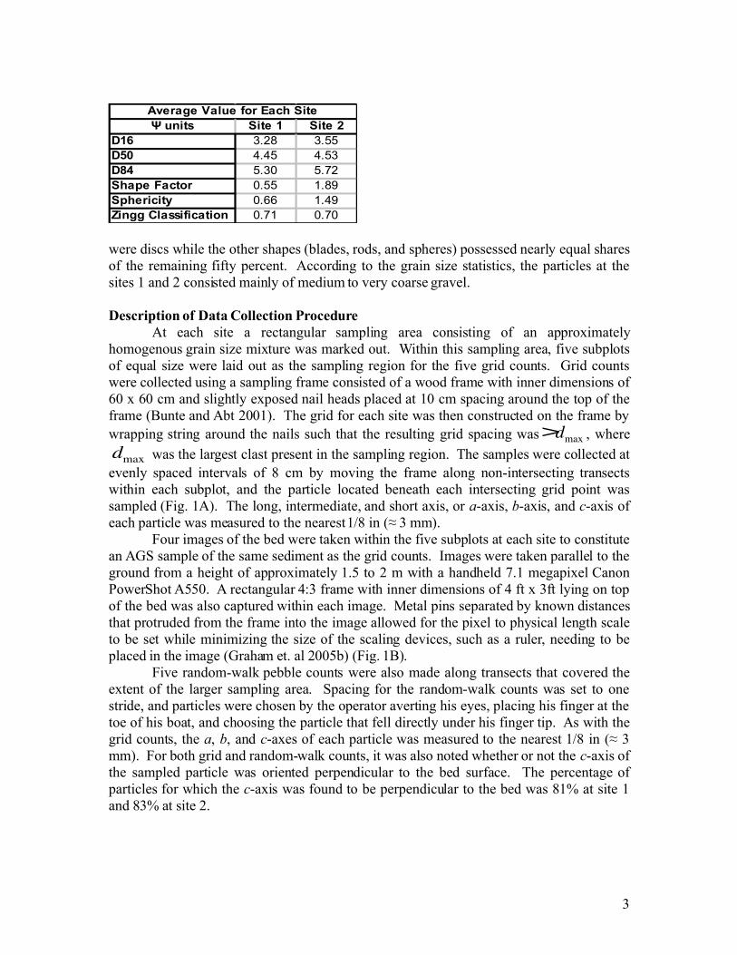
dmax was the largest clast present in the sampling region. The samples were collected at evenly spaced intervals of 8 cm by moving the frame along non-intersecting transects within each subplot, and the particle located beneath each intersecting grid point was sampled (Fig. 1A). The long, intermediate, and short axis, or a-axis, b-axis, and c-axis of each particle was measured to the nearest 1/8 in (≈ 3 mm).

Four images of the bed were taken within the five subplots at each site to constitute an AGS sample of the same sediment as the grid counts. Images were taken parallel to the ground from a height of approximately 1.5 to 2 m with a handheld 7.1 megapixel Canon PowerShot A550. A rectangular 4:3 frame with inner dimensions of 4 ft x 3ft lying on top of the bed was also captured within each image. Metal pins separated by known distances that protruded from the frame into the image allowed for the pixel to physical length scale to be set while minimizing the size of the scaling devices, such as a ruler, needing to be placed in the image (Graham et. al 2005b) (Fig. 1B).

Five random-walk pebble counts were also made along transects that covered the extent of the larger sampling area. Spacing for the random-walk counts was set to one stride, and particles were chosen by the operator averting his eyes, placing his finger at the toe of his boat, and choosing the particle that fell directly under his finger tip. As with the grid counts, the a, b, and c-axes of each particle was measured to the nearest 1/8 in (≈ 3 mm). For both grid and random-walk counts, it was also noted whether or not the c-axis of the sampled particle was oriented perpendicular to the bed surface. The percentage of particles for which the c-axis was found to be perpendicular to the bed was 81% at site 1 and 83% at site 2.

3

A BFig. 1. Images of Data Collection. A shows operators conducting a grid count sample, and B is a photo displaying the frame with metal pins used as the scaling device for the AGS method.

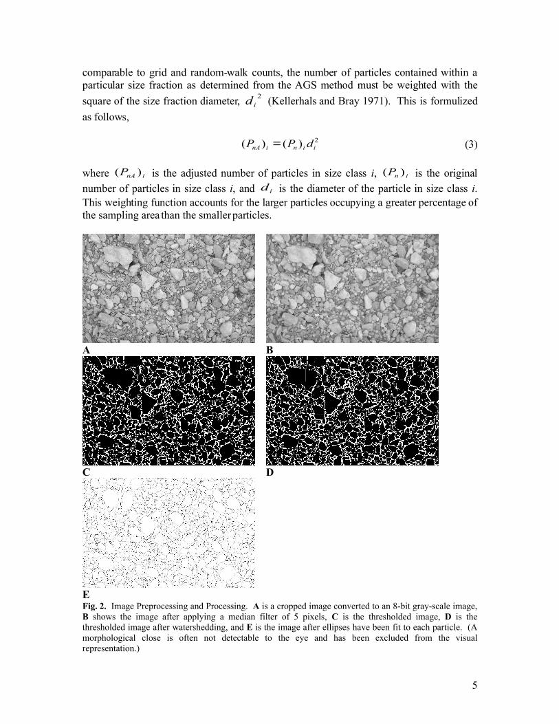
IMAGE PROCESSING PROCEDURES FOR AGSThe determination of a grain size distribution from a digital image can be organized

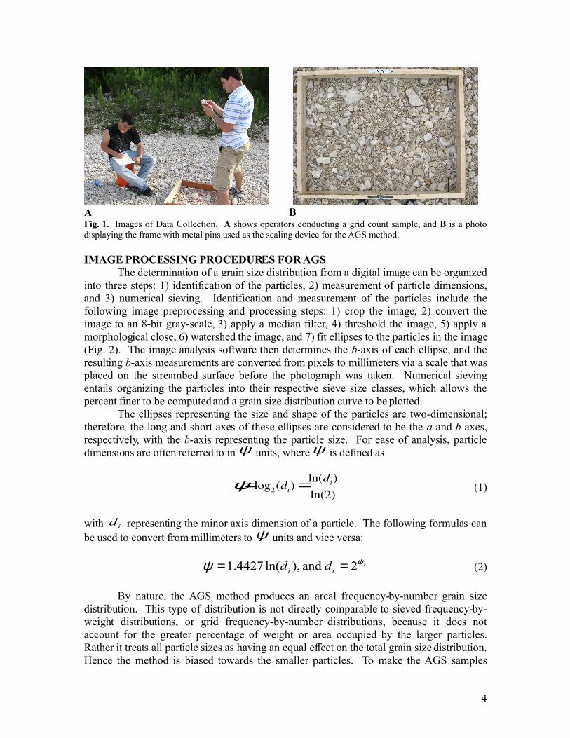
into three steps: 1) identification of the particles, 2) measurement of particle dimensions, and 3) numerical sieving. Identification and measurement of the particles include the following image preprocessing and processing steps: 1) crop the image, 2) convert the image to an 8-bit gray-scale, 3) apply a median filter, 4) threshold the image, 5) apply a morphological close, 6) watershed the image, and 7) fit ellipses to the particles in the image (Fig. 2). The image analysis software then determines the b-axis of each ellipse, and the resulting b-axis measurements are converted from pixels to millimeters via a scale that was placed on the streambed surface before the photograph was taken. Numerical sieving entails organizing the particles into their respective sieve size classes, which allows the percent finer to be computed and a grain size distribution curve to be plotted.

The ellipses representing the size and shape of the particles are two-dimensional; therefore, the long and short axes of these ellipses are considered to be the a and b axes, respectively, with the b-axis representing the particle size. For ease of analysis, particle dimensions are often referred to in ψ units, where ψ is defined as

€

ψ=log2(di) =ln(di)ln(2) (1)

with id representing the minor axis dimension of a particle. The following formulas can be used to convert from millimeters to ψ units and vice versa:

iii dd ψψ 2 and ),ln(4427.1 == (2)

By nature, the AGS method produces an areal frequency-by-number grain size distribution. This type of distribution is not directly comparable to sieved frequency-by-weight distributions, or grid frequency-by-number distributions, because it does not account for the greater percentage of weight or area occupied by the larger particles. Rather it treats all particle sizes as having an equal effect on the total grain size distribution. Hence the method is biased towards the smaller particles. To make the AGS samples

4

comparable to grid and random-walk counts, the number of particles contained within a particular size fraction as determined from the AGS method must be weighted with the

square of the size fraction diameter, 2id (Kellerhals and Bray 1971). This is formulized

as follows,

2)()( iininA dPP = (3)

where inAP )( is the adjusted number of particles in size class i, inP )( is the original

number of particles in size class i, and id is the diameter of the particle in size class i. This weighting function accounts for the larger particles occupying a greater percentage of the sampling area than the smaller particles.

A B

C D

EFig. 2. Image Preprocessing and Processing. A is a cropped image converted to an 8-bit gray-scale image, B shows the image after applying a median filter of 5 pixels, C is the thresholded image, D is the thresholded image after watershedding, and E is the image after ellipses have been fit to each particle. (A morphological close is often not detectable to the eye and has been excluded from the visual representation.)

5

Optimization of the AGS Image Processing ProceduresBefore comparing the AGS method to the grid and random-walk pebble counts, the

image processing procedures used in the AGS method must first be optimized to best identify the grains in the image. Therefore, the above methodology was optimized by: 1) determining the optimal median filter value, 2) determining whether or not a histogram equalization (a.k.a. Auto Levels) function should be applied to the images; and 3) determining whether or not the image background should be subtracted from the original image before thresholding the image. All image analysis functions were completed using ImageJ, a free image analysis software developed at the National Institutes of Health (Abramoff et al. 2004).

In order to discern the effects of the previously mentioned techniques, a control dataset containing the true sizes of the particles in the image was needed to which the various AGS results could be compared. Therefore, as a control, the minor axes (or b-axes) of all visible particles in images from both sites were manually measured within the framed region using ImageJ. In this way, datasets of approximately 2000 particles per image were developed as controls for the process optimization.

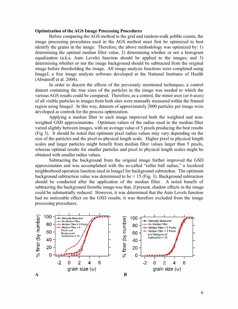
Applying a median filter to each image improved both the weighted and non-weighted GSD approximations. Optimum values of the radius used in the median filter varied slightly between images, with an average value of 5 pixels producing the best results (Fig 3). It should be noted that optimum pixel radius values may vary depending on the size of the particles and the pixel-to-physical length scale. Higher pixel to physical length scales and larger particles might benefit from median filter values larger than 5 pixels, whereas optimal results for smaller particles and pixel to physical length scales might be obtained with smaller radius values.

Subtracting the background from the original image further improved the GSD approximation and was accomplished with the so-called “roller ball radius,” a localized neighborhood operation function used in ImageJ for background subtraction. The optimum background subtraction value was determined to be ≈ 15 (Fig. 3). Background subtraction should be conducted after the application of the median filter. A noted benefit of subtracting the background from the image was that, if present, shadow effects in the image could be substantially reduced. However, it was determined that the Auto Levels function had no noticeable effect on the GSD results; it was therefore excluded from the image processing procedures.

A B

6

Fig. 3. Effect of Median Filter and Background Subtraction on GSD Results. A displays the non-weighted results, and B shows the weighted results.Manual Thresholding

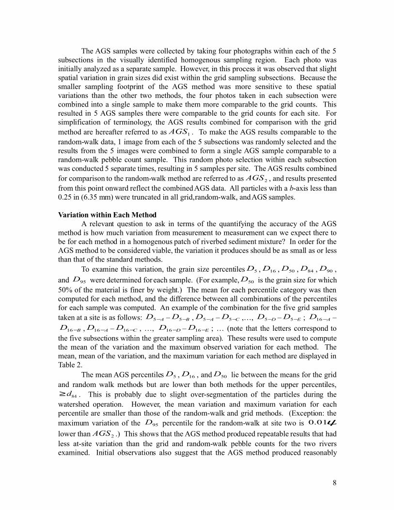
While the goal of the AGS method is to automatically detect the grains in the image with minimum user input, it was noticed that particles in images can sometime be better identified if the image threshold value is set manually rather than automatically. This process takes little time in ImageJ and users can interactively see and judge in real-time how various threshold values might effect the identification of particles. However, the use of an operator set threshold value does introduce some subjectivity. To quantify this effect, the manual threshold value was varied in steps of five beginning below and ending above the auto threshold value. These upper and lower values were chosen on the basis that an operator would not reasonably pick a higher or lower value (Fig 4). Fig. 5 shows a comparison of the grain size statistics based on the manual and auto threshold value in relation to the true grain size statistics derived from the GSD of manually measured image grains. No clear pattern for optimizing the manual thresholding technique was found. Therefore, the auto thresholding value was selected as the standard. The auto thresholding value was never optimum, but the results of the project indicate that it is sufficient.

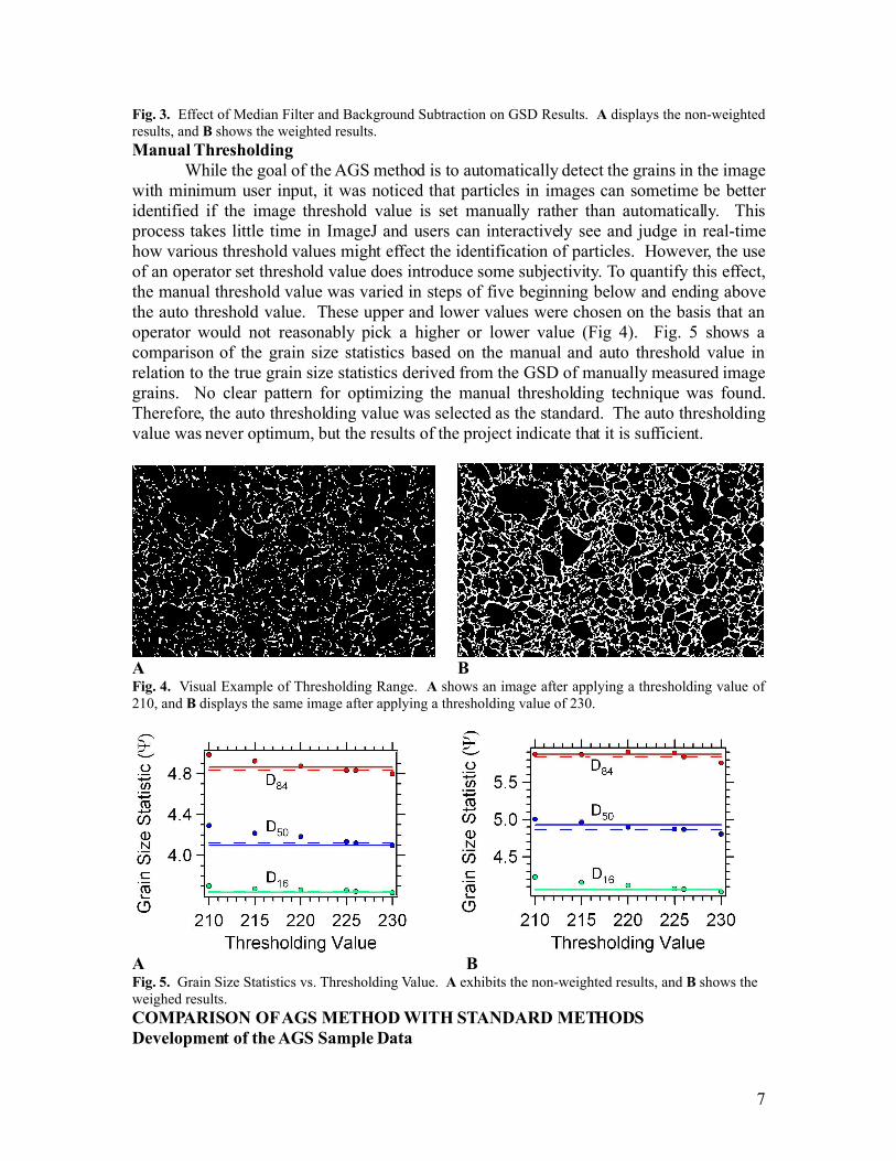
A BFig. 4. Visual Example of Thresholding Range. A shows an image after applying a thresholding value of 210, and B displays the same image after applying a thresholding value of 230.

A BFig. 5. Grain Size Statistics vs. Thresholding Value. A exhibits the non-weighted results, and B shows the weighed results.COMPARISON OF AGS METHOD WITH STANDARD METHODSDevelopment of the AGS Sample Data

7

The AGS samples were collected by taking four photographs within each of the 5 subsections in the visually identified homogenous sampling region. Each photo was initially analyzed as a separate sample. However, in this process it was observed that slight spatial variation in grain sizes did exist within the grid sampling subsections. Because the smaller sampling footprint of the AGS method was more sensitive to these spatial variations than the other two methods, the four photos taken in each subsection were combined into a single sample to make them more comparable to the grid counts. This resulted in 5 AGS samples there were comparable to the grid counts for each site. For simplification of terminology, the AGS results combined for comparison with the grid method are hereafter referred to as 1AGS . To make the AGS results comparable to the random-walk data, 1 image from each of the 5 subsections was randomly selected and the results from the 5 images were combined to form a single AGS sample comparable to a random-walk pebble count sample. This random photo selection within each subsection was conducted 5 separate times, resulting in 5 samples per site. The AGS results combined for comparison to the random-walk method are referred to as 2AGS , and results presented from this point onward reflect the combined AGS data. All particles with a b-axis less than 0.25 in (6.35 mm) were truncated in all grid, random-walk, and AGS samples.

Variation within Each MethodA relevant question to ask in terms of the quantifying the accuracy of the AGS

method is how much variation from measurement to measurement can we expect there to be for each method in a homogenous patch of riverbed sediment mixture? In order for the AGS method to be considered viable, the variation it produces should be as small as or less than that of the standard methods.

To examine this variation, the grain size percentiles 5D , 16D , 50D , 84D , 90D ,

and 95D were determined for each sample. (For example, 50D is the grain size for which 50% of the material is finer by weight.) The mean for each percentile category was then computed for each method, and the difference between all combinations of the percentiles for each sample was computed. An example of the combination for the five grid samples taken at a site is as follows: AD −5 – BD −5 , AD −5 – CD −5 ,…, DD −5 – ED −5 ; AD −16 –

BD −16 , AD −16 – CD −16 , …, DD −16 – ED −16 ; … (note that the letters correspond to the five subsections within the greater sampling area). These results were used to compute the mean of the variation and the maximum observed variation for each method. The mean, mean of the variation, and the maximum variation for each method are displayed in Table 2.

The mean AGS percentiles 5D , 16D , and 50D lie between the means for the grid and random walk methods but are lower than both methods for the upper percentiles,

84d≥ . This is probably due to slight over-segmentation of the particles during the watershed operation. However, the mean variation and maximum variation for each percentile are smaller than those of the random-walk and grid methods. (Exception: the maximum variation of the 95D percentile for the random-walk at site two is ψ01.0

lower than 2AGS .) This shows that the AGS method produced repeatable results that had less at-site variation than the grid and random-walk pebble counts for the two rivers examined. Initial observations also suggest that the AGS method produced reasonably

8

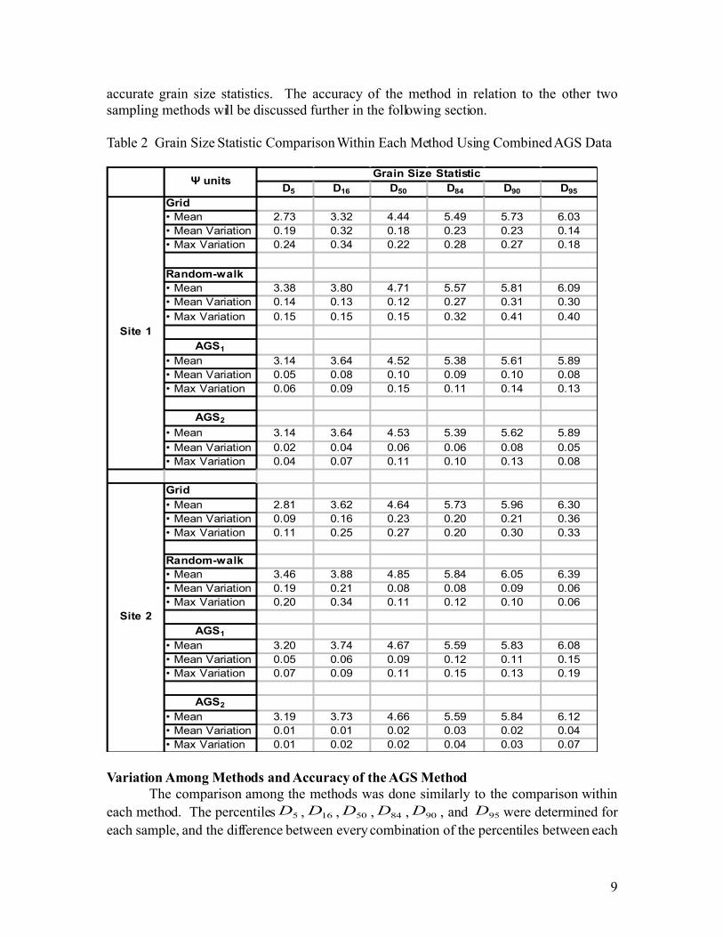
accurate grain size statistics. The accuracy of the method in relation to the other two sampling methods will be discussed further in the following section.

Table 2 Grain Size Statistic Comparison Within Each Method Using Combined AGS Data

D5 D16 D50 D84 D90 D95

Grid• Mean 2.73 3.32 4.44 5.49 5.73 6.03• Mean Variation 0.19 0.32 0.18 0.23 0.23 0.14• Max Variation 0.24 0.34 0.22 0.28 0.27 0.18

Random-walk• Mean 3.38 3.80 4.71 5.57 5.81 6.09• Mean Variation 0.14 0.13 0.12 0.27 0.31 0.30• Max Variation 0.15 0.15 0.15 0.32 0.41 0.40

AGS1

• Mean 3.14 3.64 4.52 5.38 5.61 5.89• Mean Variation 0.05 0.08 0.10 0.09 0.10 0.08• Max Variation 0.06 0.09 0.15 0.11 0.14 0.13

AGS2

• Mean 3.14 3.64 4.53 5.39 5.62 5.89• Mean Variation 0.02 0.04 0.06 0.06 0.08 0.05• Max Variation 0.04 0.07 0.11 0.10 0.13 0.08

Grid• Mean 2.81 3.62 4.64 5.73 5.96 6.30• Mean Variation 0.09 0.16 0.23 0.20 0.21 0.36• Max Variation 0.11 0.25 0.27 0.20 0.30 0.33

Random-walk• Mean 3.46 3.88 4.85 5.84 6.05 6.39• Mean Variation 0.19 0.21 0.08 0.08 0.09 0.06• Max Variation 0.20 0.34 0.11 0.12 0.10 0.06

AGS1

• Mean 3.20 3.74 4.67 5.59 5.83 6.08• Mean Variation 0.05 0.06 0.09 0.12 0.11 0.15• Max Variation 0.07 0.09 0.11 0.15 0.13 0.19

AGS2

• Mean 3.19 3.73 4.66 5.59 5.84 6.12• Mean Variation 0.01 0.01 0.02 0.03 0.02 0.04• Max Variation 0.01 0.02 0.02 0.04 0.03 0.07

Grain Size Statistic

Site 1

Site 2

Ψ units

Variation Among Methods and Accuracy of the AGS MethodThe comparison among the methods was done similarly to the comparison within

each method. The percentiles 5D , 16D , 50D , 84D , 90D , and 95D were determined for each sample, and the difference between every combination of the percentiles between each

9

sampling method was computed. For example, the difference between the five grid and random-walk (RW) samples at a site were calculated as follows: GridAD −−5 –

walkRandomAD −−−5 , GridAD −−5 – walkRandomBD −−−5 ,…, GridED −−5 –

walkRandomED −−−5 ; GridAD −−16 – walkRandomAD −−−16 , GridAD −−16 –

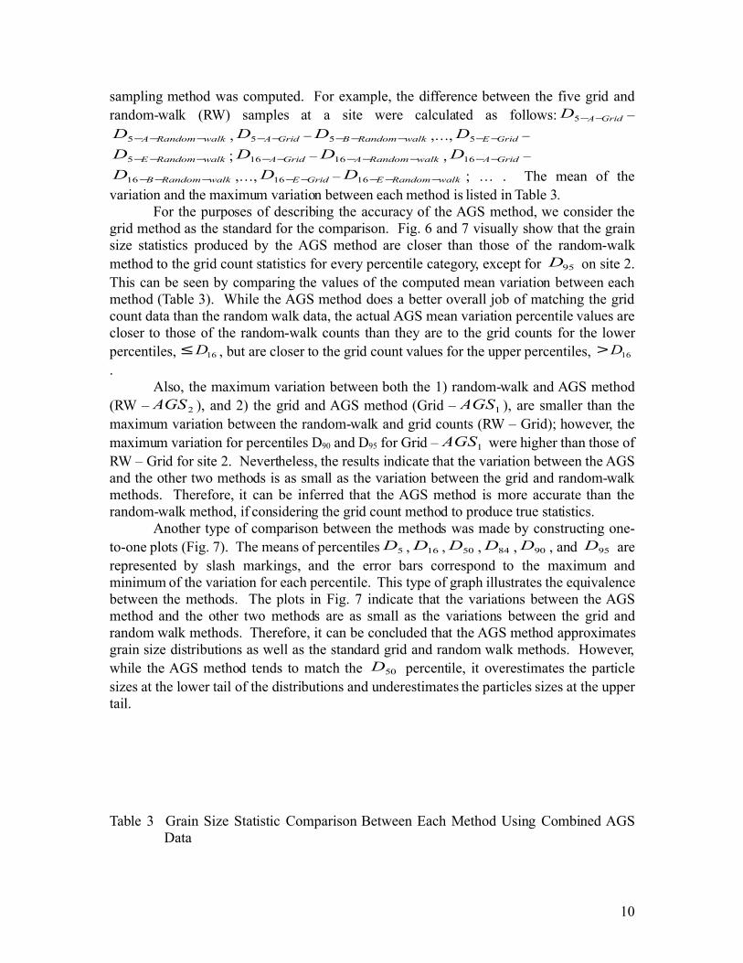
walkRandomBD −−−16 ,…, GridED −−16 – walkRandomED −−−16 ; … . The mean of the variation and the maximum variation between each method is listed in Table 3.

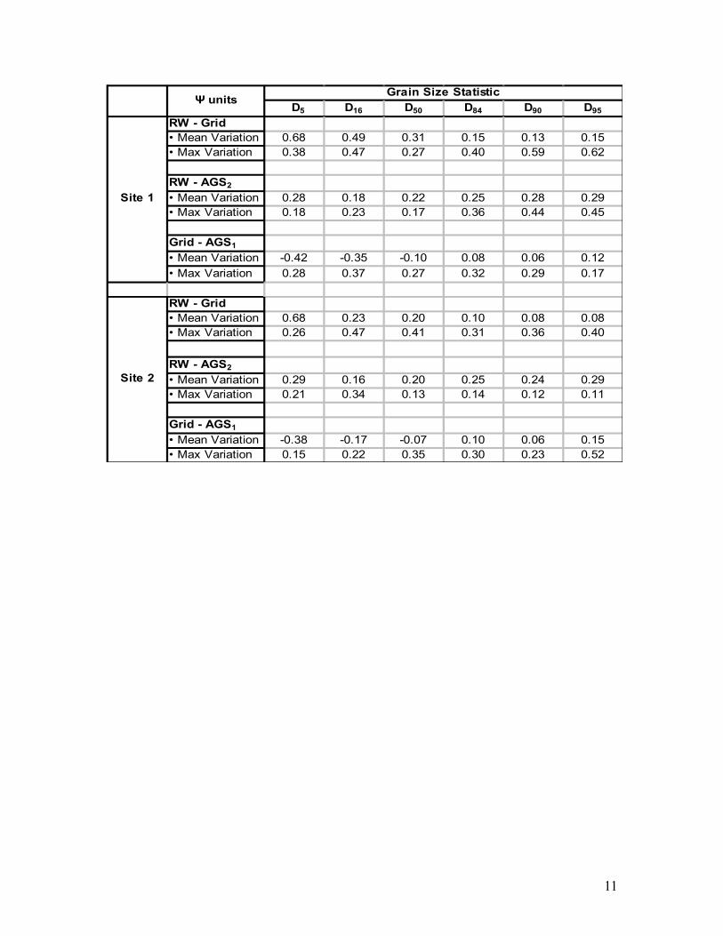
For the purposes of describing the accuracy of the AGS method, we consider the grid method as the standard for the comparison. Fig. 6 and 7 visually show that the grain size statistics produced by the AGS method are closer than those of the random-walk method to the grid count statistics for every percentile category, except for 95D on site 2. This can be seen by comparing the values of the computed mean variation between each method (Table 3). While the AGS method does a better overall job of matching the grid count data than the random walk data, the actual AGS mean variation percentile values are closer to those of the random-walk counts than they are to the grid counts for the lower percentiles, 16D≤ , but are closer to the grid count values for the upper percentiles, 16D>.

Also, the maximum variation between both the 1) random-walk and AGS method (RW – 2AGS ), and 2) the grid and AGS method (Grid – 1AGS ), are smaller than the maximum variation between the random-walk and grid counts (RW – Grid); however, the maximum variation for percentiles D90 and D95 for Grid – 1AGS were higher than those of RW – Grid for site 2. Nevertheless, the results indicate that the variation between the AGS and the other two methods is as small as the variation between the grid and random-walk methods. Therefore, it can be inferred that the AGS method is more accurate than the random-walk method, if considering the grid count method to produce true statistics.

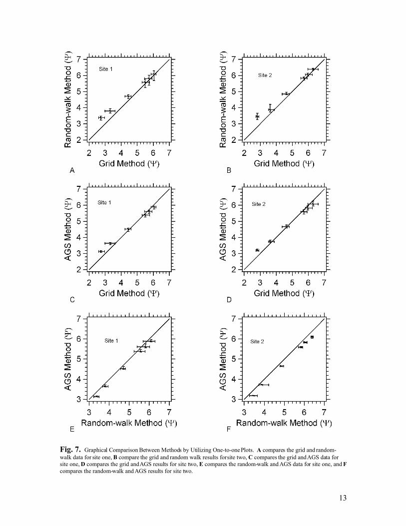
Another type of comparison between the methods was made by constructing one-to-one plots (Fig. 7). The means of percentiles 5D , 16D , 50D , 84D , 90D , and 95D are represented by slash markings, and the error bars correspond to the maximum and minimum of the variation for each percentile. This type of graph illustrates the equivalence between the methods. The plots in Fig. 7 indicate that the variations between the AGS method and the other two methods are as small as the variations between the grid and random walk methods. Therefore, it can be concluded that the AGS method approximates grain size distributions as well as the standard grid and random walk methods. However, while the AGS method tends to match the 50D percentile, it overestimates the particle sizes at the lower tail of the distributions and underestimates the particles sizes at the upper tail.

Table 3 Grain Size Statistic Comparison Between Each Method Using Combined AGS Data

10

D5 D16 D50 D84 D90 D95

RW - Grid• Mean Variation 0.68 0.49 0.31 0.15 0.13 0.15• Max Variation 0.38 0.47 0.27 0.40 0.59 0.62

RW - AGS2

• Mean Variation 0.28 0.18 0.22 0.25 0.28 0.29• Max Variation 0.18 0.23 0.17 0.36 0.44 0.45

Grid - AGS1

• Mean Variation -0.42 -0.35 -0.10 0.08 0.06 0.12• Max Variation 0.28 0.37 0.27 0.32 0.29 0.17

RW - Grid• Mean Variation 0.68 0.23 0.20 0.10 0.08 0.08• Max Variation 0.26 0.47 0.41 0.31 0.36 0.40

RW - AGS2

• Mean Variation 0.29 0.16 0.20 0.25 0.24 0.29• Max Variation 0.21 0.34 0.13 0.14 0.12 0.11

Grid - AGS1

• Mean Variation -0.38 -0.17 -0.07 0.10 0.06 0.15• Max Variation 0.15 0.22 0.35 0.30 0.23 0.52

Grain Size Statistic

Site 1

Site 2

Ψ units

11

Fig. 6. Graphical Comparison Between Methods by Utilizing Grain Size Distribution Curves. A compares the grid and random-walk data for site one, B compare the grid and random walk results for site two, C compares the grid and AGS data for site one, D compares the grid and AGS results for site two, E compares the random-walk and AGS data for site one, and F compares the random-walk and AGS results for site two.

12

Fig. 7. Graphical Comparison Between Methods by Utilizing One-to-one Plots. A compares the grid and random-walk data for site one, B compare the grid and random walk results for site two, C compares the grid and AGS data for site one, D compares the grid and AGS results for site two, E compares the random-walk and AGS data for site one, and F compares the random-walk and AGS results for site two.

13

CONCLUSIONSThis study examined the accuracy of an automated grain sizing method as

compared to standard grid and random-walk pebble counts. Image analysis techniques were explored and optimized to enhance the ability of the AGS method to identify grains in the image. The results indicate that the AGS method is at least as accurate in measuring grain size distributions as the standard random-walk pebble counts when compared to grid counts. From the study, the following conclusions are made:

1. The grain size distribution of a streambed can be determined using the automated grain sizing method for rivers with similar sediment as that examined in this study. It is expected that the grain size statistics derived from the AGS method will have less variation in the derived grain size statistics than either grid or random-walk pebble counts, and will have an accuracy at least as good, if not better, than random-walk pebble counts.

2. In comparison to grid count derived percentiles, the AGS method tends to match the median grain sizes, 50D , overestimate the size of the smallest size fractions, 16D≤ ,

and slightly underestimate the size of the largest size fractions, 84D≥ . 3. The free software package ImageJ is sufficient for analyzing digital photographs of

streambeds and in calculating accurate and precise results. This helps make the AGS method an inexpensive sampling scheme that anyone can use.

4. Applying a median filter with a radius of 5 pixels and subtracting the background based on a neighborhood operator with a radius of 15 pixels improves the results of the calculated grain size distribution. However, leveling, or histogram equalization, has a minimal or no effect. These findings are in accord with those of Graham et al. (2005a).

5. Determining a standard means for manually thresholding images will require more research. However, auto thresholding can presently be used to standardize the thresholding step in the image analysis process. Based on the results of this research, selecting the auto thresholding value resulted in the AGS method being as precise and accurate as the current standard methods; therefore, the auto thresholding value is sufficient.

While the AGS method performed quite well, it does have limitations. While not reported in this paper, the method was tested on images containing particles with a great deal of surface texture variation, such as pits, grooves, and holes and did not work well. In these cases, significant over-segmentation of larger grains was severe enough to cause the method to inaccurately measure the larger percentiles. Other than the physical constraints of deriving grain size distributions from images of the bed surface, the major issue that should be addressed in future research is finding ways to reduce over-segmentation of larger grains. Additionally, AGS techniques should be compared to standard sampling methods for a greater range of sediment sizes, shapes, and textures. This will better quantify the range of applicability of the AGS method and enable the development of sampling and processing protocols for various types, or families, or sediment mixtures.

ACKNOWLEDGEMENTS

14

The authors would like to thank Channing Santiago for his assistance in collecting field data. The research study described herein was sponsored by the National Science Foundation under the Award No. EEC-0649163 and the Department of Civil Engineering at the University of Houston. The opinions expressed in this study are those of the authors and do not necessarily reflect the views of the sponsor.

REFERENCESAbramoff, M.D., Magelhaes, P.J., Ram, S.J. (2004), "Image Processing with ImageJ".

Biophotonics International, volume 11, issue 7, pp. 36-42.Bunte, K., Abt, S. R. (2001). “Sampling Surface and Subsurface Particle-Size Distributions

in Wadable Gravel- and Cobble-Bed Streams for Analyses in Sediment Transport, Hydraulics, and Streambed Monitoring,” United States Department of Agriculture, Forest Service, General Technical Report RMRS-GTR-74.

Butler, J. B., Lane, S. N., Chandler, J. H. (2001). “Automated Extraction of Grain-size Data from Gravel Surfaces Using Digital Image Processing,” Journal of Hydraulic Research, 39(4), 519 – 529.

Church, M. A., McLean, D. G., Wolcott, J. F. (1987). “River Bed Gravels: Sampling and Analysis,” Sediment Transport in Gravel-Bed Rivers, in Thorne, C. R., Bathurst, J. C., Hey, R. D. (eds.), John Wiley and Sons, Chichester, p. 43 – 88.

Graham, D. J., Reid, I., Rice, S. P. (2005a). “Automated Sizing of Coarse-Grained Sediments: Image-Processing Procedures,” Mathematical Geology, 37(1), 1 – 28.

Graham, D. J., Rice, S. P., Reid, I. (2005b). “A Transferable Method for the Automated Grain Sizing of River Gravels,” Water Resources Research, 41, W07020, doi:10.1029/2004WR003868.

Kellerhals, R., Bray, D. I. (1971). “Sampling Procedures for Coarse Fluvial Sediments,” Proc. Am. Soc. Civ. Engrs, Journal of Hydraulics Division, 97(HY8), 1165 – 1180.

Sime, L. C., Ferguson, R. I. (2003). “Information on Grain Sizes in Gavel-bed Rivers by Automated Image Analysis,” Journal of Sedimentary Research, 73(4), 630 – 636

Wolman, M.G. (1954). “A Method of Sampling Coarse River-Bed Material,” American Geophysical Union, Transactions, 35, 951-956.

15