Comparison of different methods for measuring thermal

properties of soil: review on laboratory, in-situ and

numerical modeling methods

Hamed Hoseinimighani

Budapest University of Technology and Economics, Budapest, Hungary, hamed.h.mighani@epito.bme.hu

Janos Szendefy

Budapest University of Technology and Economics, Budapest, Hungary, szendefy@mail.bme.hu

ABSTRACT: Nowadays, development of technology and industry and arising of new engineering application, such as

nuclear waste disposal, oil extraction and pipeline, geothermal structures are encouraging the researchers to have a better

understanding about the temperature effect in soil up to 100 °C and even more when dealing with the thermal treatment

of contaminated soils. A key challenge in problems dealing with temperature is to measure the thermal properties of the

soil. Lack of such knowledge might lead to malfunction or non-economical design of structures dealing with temperature

change. Different methods can be used for determination of soil thermal properties. Each method has its own positive and

negative points comparing to other ones. Laboratory tests is a fast and economical method but meanwhile several aspects

cannot be accounted during the test. In-situ measurements is a good way to calculate soil thermal properties with respect

to actual site condition and natural environment. However it might be time consuming and expensive for particular loca-

tions and high-level technology apparatus might be required. Experimental, empirical and mathematical modeling could

a good alternative having no need for small-scale or big-scale tests however; a few models can be utilized for different

conditions and type of soils. In addition, some of these numerical models are too complex, need lots of parameters, and

can be used for specific occasions. In this paper, different methods for measurement of soil thermal properties are inves-

tigated and compared to each other including recently developed methods. Accurate measurement of soil thermal prop-

erties could help us to have a sufficient and cost effective design for engineering application dealing with temperature

change.

Keywords: soil thermal properties, thermal properties measurement, laboratory methods, in-situ measurement, prediction

models

1. Introduction

Temperature change and its potential effect on soil

properties and behavior has become an important part of

many engineering design and applications. It started at

mid-20th century when Gary[1] did the first odometer test

at different temperature of 10 and 20 °C in 1936. Paswell

[2] conducted heating test at constant load using odome-

ter ring in 1967and the first conference with focus on

temperature related issues in soils was held in Washing-

ton DC USA in 1969. The early studies of other research-

ers can be found in literature [3–14].

The range of temperature was being investigated back

then during early suited was restricted (usually between

10 to 50 °C). The reason of such limitation was related to

the researcher’s interest, which was the temperature dif-

ference between the laboratory and the field where the

samples were being taken. Nowadays, However, devel-

opment of technology and industry has caused new and

more complicated engineering application to arise, such

as nuclear waste disposal, oil extraction and pipeline and

geothermal structures which are encouraging the re-

searchers to have a better understanding about the tem-

perature effect in soil up to 100 °C and even more when

dealing with the thermal treatment of contaminated soils.

Ability of clayey soils like seepage control, pollution

prevention, heat insulation and radiation protection could

make it an ideal environment for nuclear waste disposal

[15, 16]. On the other hand, it can cause the soil to face

temperature change up to 100 °C because of chemical re-

actions of the waste. Thus, the importance of soil behav-

ior toward temperature change made many researchers to

work in this field to have better and safe design in long-

term function of these disposal areas.

Another engineering application involving tempera-

ture change is waste management and design of landfills.

Geosynthetic clay liner (GCL) is often used as a mechan-

ical and hydraulic barrier to ensure both safety of the de-

sign (e.g. in slopes) and prevention of leakage of chemi-

cal and hazardous substances and fluid into environment.

GCL is a layer of bentonite captured between layers of

geotextiles and sometimes geomemberane is used as the

final coverage for the system [17]. Chemical reactions of

wastes and temperature fluctuation of climate change can

cause the sounding area including GCL to face elevated

temperature [18–20] which might cause alternation of

mechanical and hydraulical properties of bentonite inside

the GCL and even the whole barrier system [21, 22]. for

instance rise of temperature up to 50 °C in copper leach

pads [23], 70 °C in nickel leach pads [24], 60 °C in mu-

nicipal wastes [25] and even more than 100 °C in alumi-

num waste [26] has been reported.

In recent years, pollution and Global warming related

issues and the proven effect of fossil energy on that as

well as the price in developing or even developed coun-

tries, have lead the attention toward finding a renewable

Figure 1. Horizontal and vertical GHE (a) Common vertical GHE

designs – single U-tube, (b) double U-tube, (c) simple coaxial,

(d) complex coaxial, (e) overlapping slinky loops, (f) vertical

spiral loops [29].

Figure 2. Energy pile

and sustainable source of energy such as Geothermal

Energy [27–31].

Among different type of the geothermal structures,

Ground-source heat pump (GSHP) is the most common

type for space heating and cooling [27, 29, 32–36].

GSHPs are connected to a network of buried tubes, called

ground heat exchanger (GHE), through which the water

is being circulated (Fig.1) [29, 31, 33]. Due to high exca-

vation costs especially for vertical GHEs, another type of

heat exchanger has become popular called energy piles.

A network of tubes is placed inside the pile foundation to

make a both mechanical and geothermal structure (Fig.2)

[27, 29, 31, 33, 37].

Because of soil and ground being the source of energy

in geothermal structures, it is of high importance to have

sufficient knowledge about the ground temperature pro-

file and thermal properties. Therefore several in-situ, la-

boratory and numerical studies has been done regarding

temperature profile and its thermal properties such as

thermal conductivity and diffusivity ([34, 35, 38–40]).

Heat pump function and circulation of fluid through the

soil foundation will cause the temperature fluctuation on

pile-soil interface, pile and the sounding soil. the first ex-

periment regarding this issue was done by Morino and

Oka [41].

The importance of the temperature and its possible ef-

fects on physical and mechanical properties of soil has

been highlighted by some example of engineering appli-

cations mentioned above. Sufficient knowledge on ther-

mal properties of soil is essential to have better under-

standing about the effect of temperature change on

physical and mechanical behavior of soil. The aim of this

paper is to make a detailed review and summarization

about the soil thermal properties and different methods of

measurement. This information is of high importance and

can help us to make sure about the quality and safety of

designing the structures dealing with temperature

change.

2. Thermal properties of soil

Existence of temperature difference between two

places will cause heat to transfer from the location with

higher temperature toward the lower temperature. Heat

can transfer by three method namely conduction, convec-

tion and radiation [42]. Heat transfer through geomateri-

als (soil and rock) is dominated by conduction and the

share of other heat transfer methods are negligible. Thus,

thermal properties of soil affecting the heat transfer are

important to have better idea about temperature and its

change on soil behavior [43–45].

2.1. Thermal Conductivity

According to Fourier’s law, thermal conductivity is

calculated as:

𝑘 =𝑞′′𝐿

∆𝑇 (1)

where k is thermal conductivity (W.m-1.K-1), qʹʹ is heat

flux (W.m-2), L is the material thickness (m) and ∆T is

temperature difference (K or °C) [42]. Thermal conduc-

tivity is the most important among other thermal proper-

ties in soil and governing heat transfer and temperature

distribution [46, 47]. Many external and internal factors

can alter the soil thermal conductivity [48–50]. Accord-

ing to [51] these factors are categorized as:

Compositional factors: soil mineral compo-

nents, particle size, shape, and gradation.

Environmental factors: The water content,

density and temperature.

Other factors: properties of soil components,

ions, salts, additives, and hysteresis effect.

Regarding soil minerals, Quartz has one of the strong

effect on overall soil thermal conductivity because it has

the highest thermal conductivity (around 8 W.m-1.K-1).

Another factor with high impact on soil thermal conduc-

tivity is water content, because of its higher thermal con-

ductivity (around 5.7 W.m-1.K-1) comparing to solid par-

ticles and air.

Zhang et al. [48] investigate the influence of some factors

on thermal resistivity, r (m.K.W-1), which is inversely re-

lated to thermal conductivity. Therefore, lower thermal

resistivity means higher thermal conductivity and faster

heat transfer through the soil and Vis versa. Fig.3 shows

the effect of water content on thermal resistivity. Reduc-

tion of thermal resistivity can be noticed by

Figure 3. Thermal resistivity versus moisture content at a range of dry density: (a) clay, (b) silt, (c) fine sand, and (d) coarse sand [48, 52, 53]

Figure 4. Thermal resistivity versus dry density at a range of moisture content: (a) clay, (b) silt, (c) fine sand, and (d) coarse sand [48, 52, 53]

This behavior was attributed to difference between ther-

mal resistivity of water ( about 165 K.cm.W-1) and air

(4000 K.cm.W-1) in [48]. When water content increases

inside the soil, void areas occupied by air will be replaced

by water having rather lower thermal resistivity. Other

reason for this result is the physical contact between the

soil particles that mostly governs the heat transfer. As

water content increases, a water film will be shaped

around the particles improving the physical contacts and

heat transfers afterwards. Since the particle size and ori-

entation of sand and clay are much different, different be-

havior of thermal resistivity with water content is ob-

served [48, 52, 53].

Effect of dry density on thermal resistivity is shown in

Fig.4 and decrease in thermal resistivity with increase in

dry density is observed. Higher dry density will lead to

more physical contact between particles and less air in

void areas. Effect of saturation increase is displayed in

Fig.5 and Fig.6 with reduction in thermal resistivity and

increase in thermal conductivity for all type of soils. It

can be highlighted that variation of thermal resistivity for

clayey soils is much higher comparing to sand. This is

because of nature of particle size and orientation as in

sandy soils particle physical contact is low and a small

amount of water can improve it. On the other hand in

clays much more water is needed to fully occupy the con-

tact between particles [48, 52, 54].

Particle size impact on thermal resistivity can be ob-

served in Fig.7. As it is shown, higher particle size will

cause lower thermal resistivity. This is also attributed to

the physical contact and effect of particle size on that.

Moreover the thermal resistivity of rock minerals is lower

than clay minerals [48, 55].

Figure 5. Effect of saturation on thermal resistivity of soil [48, 52,

54]

Figure 6. Effect of Saturation on different type of sand thermal

conductivity [48, 52, 54]

Figure 7. Effect of particle size on thermal resistivity [48, 55]

2.2. Heat capacity

Heat capacity (C, J.K-1) is the amount of thermal en-

ergy needed to raise the temperature of a substance by 1

degree. Accordingly specific heat (cp, J.kg-1.K-1) is the

amount of energy needed to raise the temperature of unit

mass of substance by 1 degree [42]. Many researchers

calculate the specific heat of soil by summing specific

capacity of each component [43].

2.3. Thermal diffusivity

In heat transfer analysis, the ratio of the thermal con-

ductivity to the heat capacity is an important property

termed the thermal diffusivity (α, m2.s-1) [42, 43]:

𝛼 =𝑘

𝜌𝑐𝑝=

𝑘

𝐶 (2)

Where k is the thermal conductivity, ρ is the density, cp is

the specific heat and C is the heat capacity. Higher ther-

mal diffusivity of soil means that it will react faster to

thermal change in surrounding area. On the other hand

soil with lower thermal diffusivity will react slowly to the

temperature change and takes longer time to reach new

equilibrium. Thermal diffusivity is sensitive to some soil

properties such as water content, soil texture, bulk den-

sity, and organic carbon [56–58]. Thermal diffusivity pa-

rameter is considered constant during ground tempera-

ture profile modeling in [40]. Whereas it is proven in [39]

and [38] that thermal diffusivity cannot be taken as a con-

stant parameter and it is increasing with increasing in

depth. This is mostly due to change in density and struc-

ture of the soil by compaction with depth. Table.1 shows

the thermal properties of common components in soils

[51, 59].

3. Measurement of soil thermal properties

A key challenge in problems dealing with temperature

is to measure the thermal properties of the soil. Previ-

ously indicated, thermal conductivity is the most im-

portant thermal properties of soils, which dominates heat

transfer. With the knowledge of thermal diffusivity and

heat capacity, thermal conductivity can be calculated by

Eq.2.

Different methods can be used for determination of

soil thermal properties as laboratory measurement, in-

situ measurement and numerical modeling. Each method

has its own positive and negative points comparing to

other methods. Laboratory tests is a fast and economical

way to get an insight of thermal properties of the soil but

meanwhile several aspects cannot be accounted during

the test such as effect of water movement, climate

changes and etc. thermal properties of soil are changing

with depth therefore a few samples may not be an accu-

rate represented of the actual location and environment

of the soil. Moreover, the effect of the disturbance of the

soil during sampling could be another disadvantage. In-

situ measurements is a good way to calculate soil thermal

properties with respect to actual site condition and natural

environment. However it might be time consuming and

expensive for particular locations and high-level –tech-

nology apparatus might be required. Many researchers

nowadays have been trying to calculate thermal proper-

ties of soils with experimental, empirical and mathemat-

ical modeling. Although with help of this method there is

no need for small-scale or big-scale tests, a few models

can be utilized for different conditions and type of soils.

In addition, some of these numerical models are too com-

plex, need lots parameters, and can be used for specific

occasions.

3.1. Laboratory tests

Two common type of laboratory test used by researchers

are namely steady state methods (divided bar test) and

transient method ( needle probe test) (Fig.8) [43, 45, 46,

53]. Steady state methods causes a constant temperature

gradient through the soil sample and the heat flux reaches

a constant level while, in transient methods a radial heat

flux is used and the temperature change with time

through the soil sample is measured. Each method has its

own advantages and simplification. A comparison of

these two methods is assessed on soft Bangkok clay in

[76] and the thermal conductivity changes with porosity

is shown in Fig.9. Heat flux is in one-way direction in

steady state method and it can be either horizontal or ver-

tical indicated in Fig.9. As it was discussed before ther-

mal conductivity decrease with increase in porosity and

this behavior can be observed in soft Bangkok clay too.

Although the needle probe test (Transient methods)

shows higher value of thermal conductivity comparing to

divided bar test (steady state). This behavior was ob-

served by previous works too and it has been attributed

mostly to the sample size and the difference of heat flow

between these two methods [60, 61].

Dealing with more coarse materials like gravel, a new

laboratory measurement was introduced recently in [62].

As indicated by the authors, previous works on measur-

ing gravel thermal conductivity faced some difficulties

regarding to the grain size and minerals variability be-

lieved to alter the results [63, 64]. A new apparatus is de-

veloped that could overcome the mentioned obstacles be-

cause of its large measuring surface and higher capacity.

Fig. 10 shows the developed device and the result of

measuring thermal conductivity of coarse materials.

3.2. In-situ measurements

In-situ measurement could be a reliable method to

evaluate thermal properties of soil and ground consider-

ing the natural environmental without disturbance of soil.

Thermal response test (TRT) is one of the most common

in-situ methods [30–32, 36, 65]. It was first introduced

by Mogensen and was being developed in Europe and

USA simultaneously in 90s. [30, 66, 67]. TRT method is

based on function of a pilot GHE (ground heat ex-

changer) and single or double vertical U-Tube is used to

circulate fluid through the ground (Fig.11). The circulat-

ing fluid is warmed up with constant rate of heating and

affect the temperature of borehole and surrounding soil.

This experiment is often run for 48 hours and inlet and

outlet fluid temperature is being measured continuously.

With some correlation methods, the thermal properties of

borehole and surrounding soil such as borehole thermal

resistance and soil thermal conductivity are calculated.

Advantages of

TRT is consideration of the natural state of the soil and

the geometry of a GHE that makes it a reliable method

for designing the GSHPs and geothermal structures.

Whereas some limitation and simplification will lead to

errors in thermal properties measurement such as water

movement, inhomogeneity of soil, error in sensors, volt-

age fluctuation in heater and climate and air temperature

effect. It is suggested that 5-50% error in thermal conduc-

tivity estimation can lead to 5-24% change in GHE length

and inefficient design of geothermal structure[31, 68–

71].

Jensen-Page et al. [31] studied the effect of seasonal

temperature change on the TRT performance and alter-

nation of result by seasonal temperature change was ob-

served. They found out that TRT conduction in winter

might lead to undersize design of the GHE length and

oversize design by summer TRT test. They also sug-

gested to the impact of temperature fluctuation impact on

length of GHE to be greater than 10%, the TRT should

be done in rather extreme condition and with length of

the borehole less than 35m and this impact is important

for large projects with many GHEs. On normal weather

condition and climate, the impact on GHE length is ex-

pected to be less than 5%. Many modifications have been

proposed by researchers to overcome the uncertainties of

TRT both in the way of apparatus and result analysis.

Thermal response test usually leads to calculate the

borehole thermal resistance (Rb) and effective thermal

conductivity of the surrounding soil without taking into

consideration different thermal properties for each soil

layer. With addition of distributed temperature sensing

(DTS) system, Hikari et al. [72] proposed the distributed

thermal response test (DTRT) to include the change of

thermal conductivity for each layer. Zhang et al. [65]

studied the thermal properties of ground based on DTRT

Table 1. Thermal properties of common components in soil [51, 59]

Materials Density (kg.m-3) Heat capacity (KJ.kg-1.K-1)

Thermal conductivity (W.m-1.K-1)

Thermal diffusivity (m2.s-1)×107

Air (10 °C) Water (25 °C)

Ice (0 °C)

Quartz Granite

Gypsum

Limestone Marble

Mica

Clay sandstone

1.25 999.87

917

2660 2750

1000

2300 2600

2883

1450 ~2270

1.00 4.20

2.04

0.73 0.89

1.09

0.90 0.81

0.88

0.88 0.71

0.026 0.59

2.25

8.4 1.70-4.00

0.51

1.26-1.33 2.80

0.75

1.28 1.60-2.10

0.21 1.43

12

43.08 ~12

4.7

~5 13

2.956

10 10-13

a)

b)

Figure 8. Experimental method to measure the thermal conductiv-

ity (a) steady state (b) transients [43, 45]

Figure 9. Comparison of thermal conductivity with steady and tran-

sient method [43]

and compared it with laboratory measurements. They

investigated the differences between in-situ and

laboratory result, reason of such difference and proposed

a correlation for improving laboratory result. Table.2

shows the discrepancy between laboratory result and in-

situ result which was attributed to factors such as water

movement and permeability by authors. With proposed

correlation on laboratory result, a better agreement with

in-situ measurement is reached.

Although DTRT was able to measure the thermal

properties of layered ground accurately, it was not able to

monitor water movement and seepage. Cao et al. [30]

modified the DTRT with actively optical fiber-based

technology, developed for in-situ moisture measuring

with interpreting the relation between temperature

change and moisture, and proposed Active distributed

thermal response test (A-DTRT) based on active distrib-

uted temperature sensing (A-DTS) systems to investigate

the effect of moisture movement on thermal conductivity.

a)

b)

Figure 10. New laboratory test methodology for Gravel and Coarse

materials (a) developed apparatus (b) experimental results [62]

Figure 11. Schematic view of Thermal Response Test [36]

Table 2. Comparison between in-situ and laboratory of thermal con-

ductivity (W.m-1.K-1) [65]

layer In-situ Laboratory before

modification

Laboratory after

modification

Grit 1.906 1.362 1.825

Silty clay 1.397 1.143 1.404

Sandstone 2.854 2.220 2.778

Mudstone 1.520 1.432 1.689

Fig.12 shows distributed thermal conductivity along

the borehole length and difference between laboratory

and in-situ result support the need for a correlation as pro-

posed before in [65]. It is also observed that laboratory

thermal conductivity of soil is lower than in-situ results.

However, the thermal conductivity of rocks in laboratory

lead to higher value comparing to in-situ results.

Figure 12. Thermal conductivity of layered ground [30]

Authors believed that water loss and structure change in

soil sample and the existence of cracks in field rocks are

the reasons for such differ ences. For the effect of mois-

ture on the thermal conductivity result, a critical moisture

(βcr) was introduced. For β<βcr the effect of water move-

ment on TRT results are negligible whereas for β>βcr the

real time monitoring of water movement and possible

modification of the test should be considered. Fig.13

shows the effect of seepage velocity on thermal conduc-

tivity. Increase in velocity causes the thermal conductiv-

ity in ground to increase too and when velocity increases

from 0 to 1.6 the thermal conductivity will increase from

2.2 to 14.3 W.m-1.K-1. This suggests that area with higher

seepage velocity are preferred for the location of GSHPs

and GHEs.

Common models for analysis the recorded tempera-

ture with TRT to calculate thermal properties is infinite

line source model (ILSM). According to the model, the

BHE is considered as an infinitely long line source lo-

cated in a homogeneous, isotropic and infinite medium,

which regression fit to the measured data curve between

mean circulating fluid temperatures is further used to de-

termine the effective thermal conductivity of the subsur-

face. Then thermal diffusivity can be calculated by divid-

ing thermal conductivity into average heat capacity of

subsurface layers [36]. More advanced methods has pro-

posed by researchers to drive thermal properties from

measure temperature data. Li et al. [46] proposed a least

square method based on Finite elements ( FELSM) to

measure thermal conductivity. They also validates the

FELSM results by predicting the temperature and com-

paring it with laboratory temperature distribution through

a sample. Fig.14 shows the high accuracy on the pro-

posed method.

Akhmetov et al. [36] integrated borehole temperature

relaxation method (BTR) into conventional TRT. They

found out the depth average thermal conductivity based

on BTR method is about 0.45 W.m-1.K-1 which is almost

3 times lower that thermal conductivity based on LSM

(1.56 W.m-1.K-1). This was attributed by the authors to

heat convective loss to the ground surface at depth 9-16m

that was not considered in LSM method. BTR could also

show the depth dependency of thermal conductivity.

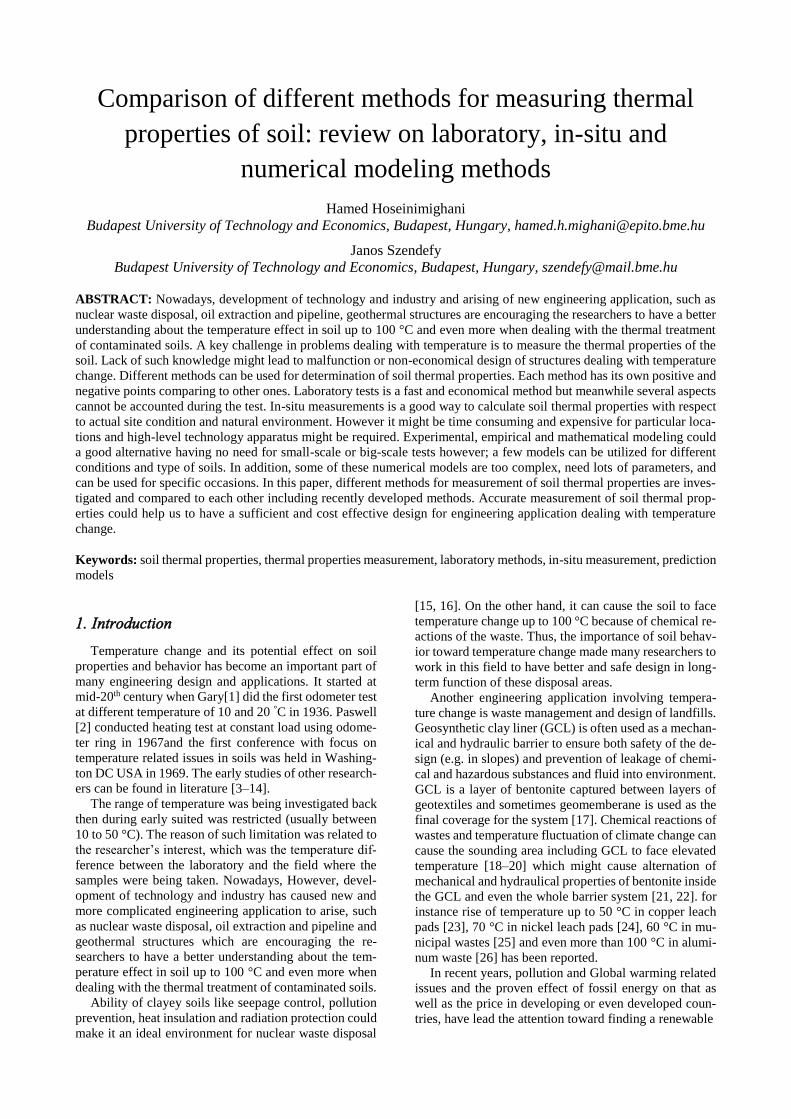
Other techniques has also been introduced by re-

searcher for in-situ measurement of thermal properties of

the soil. Zhang et al. [49] integrated dual-probe heat pulse

(DPHP) device with time domain reflectometry (TDR)

technique and proposed thermo-TDR for measuring ther-

mal properties and soil moisture of four different sands at

the same time. The compared the result with three model

predictions for thermal conductivity and Fig.15 shows

the good agreement between models

Figure 13. Effect of seepage velocity on apparent thermal conduc-

tivity derived by in-situ TRT test [30]

Figure 14. Measured temperature data Vs predicted temperature by

FELSM [64]

prediction and in-situ measurements. Schematic view of

thermos-TDR is shown in Fig.16.

Lines et al. [32] integrated a soil moisture probe into

cone penetration test with pore pressure measurement

(CPTu) and proposed a newly-developed thermal cone

dissipation test (TCT) to measure soil thermal conductiv-

ity of different layers. The function of this test is based

on the temperature rise on the cone cause by the friction

and measuring the heat dissipation over the time of stop-

ping. They conducted three tests on different kind of soil

such as soft clay and stiff sandy clay. It was concluded

Figure 15. Comparison of thermal conductivity of four different

sand by model prediction and thermos-TDR [36]

that TCT is a promising, fast and economical solution to

estimate the thermal properties of the soil since CPTu is

very common geotechnical test, although there is some

limitation with the proposed test like there was not

enough temperature rise in soft clay to measure the ther-

mal properties. Authors suggested that further studies

were needed to be done to improve the device and test

procedure to make it as reliable, fast and economical ap-

paratus.

3.3. Prediction models

Laboratory and in-situ tests might be time consuming,

rather expensive in some situation and not applicable in

all conditions. Therefore, researchers have been trying to

develop theoretical and empirical models based on the in-

situ and laboratory measurements to estimate thermal

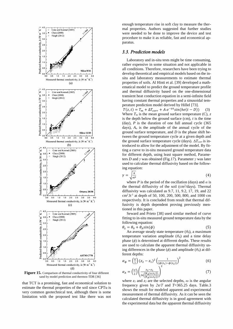
properties of soils. Al Hinti et al. [39] developed a math-

ematical model to predict the ground temperature profile

and thermal diffusivity based on the one-dimensional

transient heat conduction equation in a semi-infinite field

having constant thermal properties and a sinusoidal tem-

perature prediction model derived by Hillel [73].

𝑇(𝑧, 𝑡) = 𝑇𝑚 + ∆𝑇𝑐𝑜𝑟𝑟 + 𝐴°𝑒−𝛾𝑧𝑠𝑖𝑛 (ℎ𝑒(𝑡 − 𝐷)) (3)

Where Tm is the mean ground surface temperature (C), z

is the depth below the ground surface (cm), t is the time

(day), P is the duration of one full annual cycle (365

days), Ao is the amplitude of the annual cycle of the

ground surface temperature, and D is the phase shift be-

tween the ground temperature cycle at a given depth and

the ground surface temperature cycle (days). ∆Tcorr is in-

troduced to allow for the adjustment of the model. By fit-

ting a curve to in-situ measured ground temperature data

for different depth, using least square method, Parame-

ters D and γ was obtained (Fig.17). Parameter γ was later

used to calculate thermal diffusivity based on the follow-

ing equation:

𝛾 = √𝜋

𝛼𝑃 (4)

where P is the period of the oscillation (days) and α is

the thermal diffusivity of the soil (cm2/days). Thermal

diffusivity was calculated as 9.7, 11, 9.2, 17, 19, and 22

cm2.h-1 at depth of 50, 100, 200, 500, 800, and 1000 cm

respectively. It is concluded from result that thermal dif-

fusivity is depth dependent proving previously men-

tioned in this paper.

Seward and Prieto [38] used similar method of curve

fitting to in-situ measured ground temperature data by the

following equation:

𝜃𝑧 = 𝜃0 + 𝜃𝐴𝑠𝑖𝑛 (𝜙) (5) An average steady state temperature (θ0), a maximum

temperature variation amplitude (θA) and a time delay

phase (ϕ) is determined at different depths. These results

are used to calculate the apparent thermal diffusivity us-

ing differences in the phase (ϕ) and amplitude (θA) at dif-

ferent depths:

𝛼𝜙 = (𝜔

2) (𝑧2 − 𝑧1)2 (

1

(𝜙(𝑧1)−𝜙(𝑧2)))

2

(6)

𝛼𝐴 = (𝜔

2) (

𝑧2−𝑧1

𝑙𝑛(|𝜃𝐴(𝜔,𝑧1)|

|𝜃𝐴(𝜔,𝑧2)|))

2

(7)

where z1 and z2 are the selected depths, ω is the angular

frequency given by 2π/T and T=365.25 days. Table.3

shows the result for modeled apparent and experimental

measurement of thermal diffusivity. As it can be seen the

calculated thermal diffusivity is in good agreement with

the experimental data but the apparent thermal diffusivity

Figure 16. Thermo-TDR device [49]

Figure 17. Comparison between prediction model and in-situ measurement of ground temperature at different depth [39]

Table 3. Experimental and predicted thermal diffusivity [38]

Depth(m) Soil type

Thermal diffusivity

(×10-7 m2/s)

In-situ(αA) In-situ(αϕ) lab

0.1-1.0 Top

soil/clay 3.39 4.41 3.78

1.0-3.0 Sand-grit

clay 6.75 6.31 4.10

3.0-6.0

Clay with

sand and

pebbles

7.78 5.82 6.67

6.0-9.0 Clay with

large stones 9.92 10.6 7.95

calculated based on the maximum temperature amplitude

are closer to the experimental data and it was related by

authors to the bigger effect of inhomogeneity in the soil

on phase lag over depth than temperatures. Thermal dif-

fusivities increased with depth, as it was observed in pre-

vious mentioned study, suggesting that the ground at

depth has a greater capability for rapid changes in tem-

perature. Authors believed this is likely due to increased

saturation levels and compaction of material at depth, al-

lowing heat to be transferred quickly. As it was discussed

in section 3.2, one the limitation of in-situ measurement

techniques such as TRT is no considering the effect of

different layers which was proven in [38, 39] that ne-

glecting this issue can alter the results significantly.

Many researchers have been trying to develop mathemat-

ical models to predict thermal properties of soil during

past years. Wiener [74] theoretically proposed upper and

lower limit of thermal conductivity. Maximum and min-

imum values of thermal conductivity occurs when the

heat flow is parallel and perpendicular to components re-

spectively. These values are also called Wiener boundary

and calculated as follow:

𝑘 = 𝑘𝑤𝐿 = [∑

∅𝛼

𝑘𝛼]

−1

(Lower limit) (8)

𝑘 = 𝑘𝑤𝑈 = ∑ ∅𝛼𝑘𝛼 (Upper limit) (9)

Where ϕα and kα are the volume fraction and thermal con-

ductivity of each phase (solid, liquid and gas), respec-

tively. De Vires [75] introduced another theoretical for-

mula for thermal conductivity based on uniform

distribution of solid particles in continuous porous me-

dium as follow :

𝑘 =∑ 𝐾𝑖𝜒𝑖𝑘𝑖

𝑁𝑖=0

∑ 𝐾𝑖𝜒𝑖𝑁𝑖=0

(10)

Where ki is the thermal conductivity of each soil constit-

uent, χi is the volume fraction of each component and Ki

is the ratio of average thermal gradient of each compo-

nent to that of continuous medium in soils. De Vires pro-

posed following equation for Ki considering particle size

and shape:

𝐾𝑖 =1

3∑ [1 + (

𝑘𝑖

𝑘0− 1) 𝑔𝑎]

−1

𝑎,𝑏,𝑐 (11)

Where ga, gb and gc are the grain shape coefficients, and

usually taken as 1/3 for spherical soil particles and ki/k0

is the ratio of thermal conductivity of one soil constituent

to that of continuous medium in soils. Disadvantages of

de Vires model is that determination of parameter Ki is

somewhat difficult since it is affected by many factors.

This model consider the air and water distributed uni-

formly through the medium that might affect the result

too. Some modification based on these early studied have

also been published. Tong et al. [76] proposed a new

model to predict thermal conductivity of soil based on

Wiener model [74]. Advantage of this model is that many

influencing factors such as water content, porosity, de-

gree of saturation, temperature and pressure are consid-

ered:

𝑘 = 𝜂1(1 − 𝜙)𝑘𝑠 + (1 − 𝜂2)[1 − 𝜂2(1 − 𝜙)]2 ×

[(1−∅)(1−𝜂1)

𝑘𝑠+

𝜙𝑆𝑟

𝑘𝑤+

𝜙(1−𝑆𝑟)

𝑘𝑔]

−1

× 𝜂2[(1 − 𝜙)(1 −

𝜂1)𝑘𝑠 + 𝜙𝑆𝑟𝑘𝑤 + 𝜙(1 − 𝑆𝑟)𝑘𝑔] (12)

Where ks, kw and kg are the thermal conductivities of

solid, water and gas, respectively, ϕ is the porosity; η1 is

the parameter related to porosity, 0 < η1(ϕ) < 1; η2 is pa-

rameter related to porosity, degree of saturation and tem-

perature, 0 < η2(ϕ,Sr,T) < 1. As it was discussed in section

3.2, simplification and alternation in soil structure and

environment could cause some discrepancy between la-

boratory test and in-situ measurement for soil thermal

properties. So it is beneficial to consider influencing fac-

tors as much as it is possible. Beside the advantages of

this model, it is more complex comparing to previous

model and determination of parameters η1 and η2 should

be attended carefully. A recent theoretical model for sand

is proposed by Haigh [77] which consider the interaction

between the solid, liquid and gas during the heat conduc-

tion and gives much better result comparing to previous

models. The formulation is as follow: 𝑘

𝑘𝑠= 2(1 + 𝜉)2 {

𝛼𝑤

(1−𝛼𝑤)2 𝑙𝑛 [(1+𝜉)+(𝛼𝑤−1)𝜒

𝜉+𝛼𝑤] +

𝛼𝑎

(1−𝛼𝑎)2 𝑙𝑛 [(1+𝜉

(1+𝜉)+(𝛼𝑎−1)𝜒]} +

2(1+𝜉)

(1−𝛼𝑤)(1−𝛼𝑎)[(𝛼𝑤 −

𝛼𝑎)𝜒 − (1 − 𝛼𝑎)𝛼𝑤] (13) where k and ks are the thermal conductivities of soil and

solid, αw=kw/ks is the ratio of thermal conductivity of wa-

ter to thermal conductivity of soils, αa=ka/ks is the ratio

of thermal conductivity of gas to thermal conductivity of

soils, ξ and χ are parameters related to the water film and

degree of saturation respectively. Complexity of determi-

nation for parameter ξ and χ is disadvantages of this

model comparing to the early simpler ones. These models

are based on theoretical assumption of porous medium

however empirical fit to experimental measurements are

quite common methods to develop models to predict ther-

mal properties of soil. Kersten [78] proposed and early

simple model for soil thermal conductivity considering

water content and dry density with experimental meas-

urement on 19 samples including gravels and sands,

sandy soils and clayey soils, mineral soils and crushed

stones and organic soil :

𝑘 = 0.1442[0.9 log 𝑤 − 0.2] × 100.6243𝛾𝑑 (14) (Silt and clay)

𝑘 = 0.1442[0.7 log 𝑤 + 0.4] × 100.6243𝛾𝑑 (15) (Sandy soils)

where k is the thermal conductivity of soils, W.m-1.K-1; w

is the moisture content of soils, %; and γd is the dry den-

sity of soils, lb/ft3. Johansen [79] developed kersten

model [78] and introduced normalized thermal conduc-

tivity for the first time as follow :

𝑘𝑟 =𝑘−𝑘𝑑𝑟𝑦

𝑘𝑠𝑎𝑡−𝑘𝑑𝑟𝑦 (16)

Where ksat and kdry are the soil thermal conductivities un-

der fully saturation and dry condition respectively. Ther-

mal conductivity of soil can be calculated by knowing ksat

and kdry with the help of new kr, which is also called Ker-

sten number. For determination of ksat , Sass et al. [80]

proposed a simple formula which is widely being used by

researchers :

𝑘𝑠𝑎𝑡 = 𝑘𝑠1−𝑛𝑘𝑤

𝑛 (17) Where ksat, ks and kw are saturated, solid particles and

water thermal conductivity respectively. Porosity, n, can

be calculated as follow:

𝑛 = 1 −𝜌𝑑

𝑑𝑠𝜌𝑤 (18)

Where ρd and ρw are soil dry density and density of water

respectively and ds is relative density of solids particles.

kw is about 0.6 W.m-1.K-1 at room temperature. If the min-

eral component of soil are, know the thermal conductiv-

ity of solid particles can be calculated as follow:

𝑘𝑠 = ∏ 𝑘𝑚𝑗

𝜒𝑗𝑗

∑ 𝜒𝑗 = 1𝑗 (19)

Soils are often consist of several types of minerals that

might make it difficult to calculate the thermal conduc-

tivity of solid particles. As it was discussed previously in

this paper, Quartz has the most important effect on ther-

mal conductivity among other minerals. Therefore Jo-

hansen [79] proposed a simplified model to calculate ks

based on the Quartz content of soil :

𝑘𝑠 = 𝑘𝑞𝑞

𝑘01−𝑞

(20)

Where kq, k0 and q are thermal conductivity of Quartz,

average thermal conductivity of other minerals and vol-

ume fraction of quartz respectively. Eq.20 also could be

simplified as follow:

𝑘𝑠 = {21−𝑞 × 7.7𝑞 , 𝑞 > 0.2

31−𝑞 × 7.7𝑞 , 𝑞 ≤ 0.2 (21)

Johansen [79] also modified de Vires model [75] to

calculate thermal conductivity of dry soil :

𝑘𝑑𝑟𝑦 =0.137𝜌𝑑+64.7

2650−0.947𝜌𝑑 (22)

After determination of ksat and kdry the only remaining

parameter is kr. by fitting experimental data Johansen

[79] also proposed some equation to calculate normalized

thermal conductivity (Kersten number) based on degree

of saturation (Sr) :

𝑘𝑟 =

{

0.7 log(𝑠𝑟) + 1 𝑓𝑜𝑟 𝑚𝑒𝑑𝑖𝑎𝑛 𝑎𝑛𝑑 𝑓𝑖𝑛𝑒 𝑠𝑎𝑛𝑑

log(𝑠𝑟) + 1 𝑓𝑜𝑟 𝑓𝑖𝑛𝑒 𝑠𝑜𝑖𝑙𝑠

0.54𝑠𝑟2 + 0.46𝑠𝑟 𝑓𝑜𝑟 𝑝𝑒𝑎𝑡

(23)

Comparing to Kersten model [78] which was very

simple rather low in accuracy, Johansen model [79] gave

a better result and it has been the base for many other

models afterwards. Cote and Konrad [81] proposed a new

relationship for kr considering the effect of soil type by

using parameter κ :

𝑘𝑟 =𝜅𝑆𝑟

1+(𝜅−1)𝑆𝑟 (24)

A new equation for thermal conductivity of dry soil

was proposed based on the porosity:

𝑘𝑑𝑟𝑦 = 𝜒10−𝜂𝑛 (25)

Figure 18. Performance of thermal conductivity prediction model and experimental data [51]

Where χ and η are parameter related to effect of soil type

and grain shape respectively. Table 4 shows the value of

parameter κ, χ and η for different type of soils.

Another modification of Johansen model [79] is done by

Balland and Arp [82]. They proposed a new equation for

thermal conductivity of solids considering the effect of

organic matter:

𝑘𝑠 = 𝑘𝑜𝑚𝑉𝑜𝑚𝑘𝑞

𝑞𝑘0

1−𝑞−𝑉𝑜𝑚 (26)

Where kom and Vom are thermal conductivity and volume

fraction of organic matter respectively. They also pro-

posed following equation for the dry and normalized

thermal conductivity:

𝑘𝑑𝑟𝑦 =(𝑎𝑘𝑠−𝑘𝑎)𝜌𝑑+𝑘𝑎𝐺𝑠

𝐺𝑠−(1−𝑎)𝜌𝑑 (27)

𝑘𝑟 = 𝑆𝑟0.5(1+𝑉𝑜𝑚−𝛼𝑉𝑠𝑎𝑛𝑑−𝑉𝑠 [(

1

1 + exp (−𝛽𝑆𝑟

)3

− (1 − 𝑆𝑟

2)

3

]

1−𝑉𝑜𝑚

Where ka is thermal conductivity of air, a is constant

(~0.053), Gs is specific density, α and β are coordination

coefficient and Vsand and Vc are volume fraction of sand

and coarse material respectively. Lu et al. [83] Conducted

laboratory test using Thermo-TDR probe and proposed

following equation by empirical fit to the data:

𝑘 = [𝑘𝑤𝑛 𝑘𝑠

1−𝑛 − (𝑏 − 𝑎𝑛)] × [𝛼(1 − 𝑆𝑟𝛼−1.33)] (28)

a and b are parameter considering the thermal conductiv-

ity of dry soil and α is parameter accounting for effect of

soil type on normalized conductivity. a and b are sug-

gested to be taken as 0.56 and 0.51 respectively. For pa-

rameter α, 0.96 and 0.27 are suggested for coarse and fine

materials.

Chen et al. [84] proposed simple equation to estimate

thermal conductivity of quartz sand using thermal probe

in laboratory :

𝑘 = 𝑘𝑤𝑛 𝑘𝑠

1−𝑛[(1 − 𝑏)𝑆𝑟 + 𝑏]𝑐𝑛 (29) Where b and c are fitting parameter and value of

0.0022 and 0.78 are suggested for quartz sand respec-

tively. The accuracy of model is high for sand since it is

based on empirical fit to laboratory tests on quartz sand.

Most recently Zhang et al. [49] measured thermal con-

ductivity of sands using Thermo-TDR probe and modi-

fied the Cote and Conrad model [81]. The model is sim-

ple similar to Chen et al model [84] however the accuracy

is even higher. The comparison of modified Cote and

Conrad model performance with measured experimental

data and Chen et al [84] and Haigh [77] is shown in

Fig.15.

Table 4. Value of cote and Conrad parameters [81]

Soil type parameter

κ χ η

Well-graded gravels and coarse sands 4.60 1.70 1.80

Medium and fine sands 3.55 1.70 1.80

Silts and clays 1.90 0.75 1.20

Peat 0.60 0.3 0.87

Table 5. Suggested value for b [55]

Soil type Parameter b

Silt -0.54

Silty sand 0.12

Fine sand 0.70

Coarse sand 0.73

Mixed model using both empirical and theoretical

approaches are proposed as well. Donazzi et al. [85]

proposed following equation for thermal conductivity

prediction:

𝑘 = 𝑘𝑤𝑛 𝑘𝑠

1−𝑛 𝑒𝑥𝑝[−3.08𝑛(1 − 𝑆𝑟)2] (30) Midttomme [86] developed another model consider-

ing the effect of particle size (dm) as follow :

𝑘 = 0.215 × log(𝑑𝑚) + 1.93 (31) Gangadhara Rao and Singh [55] proposed a model

considering dry density and moisture content using nee-

dle probe test in laboratory :

𝑘 = 100.01𝛾𝑑−1(1.07 log 𝑤 + 𝑏) (32) Parameter b is to consider soil type and table.5 shows

the suggested values proposed by the authors.

Comparison between different prediction models and

experimental data in literature on thermal conductivity of

sand is studied in [51]. As it can be observed in Fig.18

most of the model predicted values are less than experi-

mental measurement because they do not usually take

into account the effect of quartz. Table.6 also show a

comparison between different model [51]. Most of the

prediction model could give good result in sand and

coarse material and usually underestimate the thermal

conductivity in fine materials. This well proved in study

of T.Zhang et al. [48]. A review on thermal conductivity

calculation procedure is proposed based on the normal-

ized thermal conductivity (kr) concept (Fig.19). the result

of proposed method is evaluated against prediction

model in two location Ninjang, China [52] and India [55].

As Fig.21 shows, there is good agreement between cal-

culated and predicted results for coarse materials how-

ever; the models underestimate the thermal conductivity

for fine-grained soils. These behaviors was attributed to

unknown mineralogy of fine soils, which is usually re-

quired complex experiments. On the other hand a good

linear relationship between predicted and calculated re-

sult for fine grained soil is seen therefore a correlation

coefficient for empirical parameters was proposed by the

authors as 1.736 and 2.415 for Ninjang and India areas

respectively. Fig.23 shows the comparison of result after

modification of empirical parameters for fine materials

and a good agreement is established. This method can

help geotechnical engineers to estimate thermal conduc-

tivity of soils and avoid mineralogy tests.

4. Conclusion

The importance of temperature change and its effect

on soil properties and behavior were brought up earlier in

this paper followed by some examples of geotechnical

application dealing with temperature change. Thus, it is

of high importance to have clear understanding about

temperature change and its possible effects on different

aspects of geotechnical designs. In order to do so, the first

important step is to measure and interpret the thermal

properties of soils which is believed to have great effect

on response of the soil to temperature change.

Different factors influencing thermal properties of the

soil were investigated by authors. It can be concluded that

water content and volume fraction of Quartz are the most

important and dominating ones. Quartz has the highest

thermal conductivity among other common soil minerals

and water has the higher thermal conductivity comparing

to other phases in soils (solid particles and air). There-

fore, they have great effect on the overall thermal con-

ductivity of the soil. Since the heat transfer in soil is gov-

erned by conduction, physical contact between particles

can affect the thermal conductivity too.

Figure 19. steps methods proposed in [48]

Table 6. Comparison between different prediction model for thermal conductivity [51]

model Advantage disadvantage Applica-

bility

wiener Quantification of two limit thermal conductivity Not applicable to soils Porous

De Vires High prediction accuracy Complex formula, difficult to determine pa-

rameters All

Tong et al. Considering many influence factors comprehensively Complex formula, difficult to determine pa-

rameters

Porous

medium

Haigh Simple formula and high prediction accuracy Limited applicability sands

Kersten Simple formula Neglect of quartz content effect All

Johansen Normalized thermal conductivity concept and relatively

high prediction accuracy

Unknown effect of soil type on kr-Sr relation-

ship All

Cote and Conrad Considering effect of soil type on kr-Sr relationship Unknown sensitivity of κ to soil type All

Balland and Arp Considering effect of organic content Neglect of quartz content in solid phase All

Lu et al. Simple formula Unknown effect of soil type on thermal con-

ductivity of dry soils All

Chen High prediction accuracy for sands with relatively high

quartz content Not applicable to other soil types sands

Zhang et al. Very high prediction accuracy for quartz sands Not applicable to other soil types Quartz

sands

Donazzi et al. Simple formula Low prediction accuracy at low saturation All

Gangadhara and

singh Simple formula Low prediction accuracy at high saturation All

Midttomme et al. Simple formula Only considering particle size effect Quartz

sands

Figure 20. Comparison of calculated and predicted thermal con-

ductivity before modification [48]

Figure 21. Comparison of calculated and predicted thermal con-

ductivity after modification [48]

Increase in properties like density, compaction and

particle size can increase the thermal conductivity by in-

creasing the physical contact between the particles. In-

crease in water content and degree of saturation can in-

crease the physical contact between particles too,

especially in fine grain soils, by creating a water layer

around the solid particles (e.g. double layer in clayey

soils). It is essential to pay closer attention to water con-

tent during measurement of thermal conductivity since its

variation can greatly alter the thermal conductivity in dif-

ferent ways.

Various methods have been used by researchers to

measure the thermal properties of the soil as laboratory

test, in-situ measurement and prediction models. Ad-

vantages and disadvantages of these methods were inves-

tigated and the following worth to be mentioned. Labor-

atory tests offers quick, easy to perform and somewhat

economical options to measure thermal conductivity.

However they are usually consider some simplifying as-

sumptions and therefore might not represent the actual

condition. Disturbance of the samples and removal from

the site might alter the structure of the soil and hence lead

to different results. As it was mentioned previously in the

paper, thermal properties could not be considered as a

constant parameters and could vary especially through

the depth because of the inhomogeneity in the ground and

small scale laboratory sample might not be a very good

represented of the actual ground. It is suggested to pay

attention to water content change during laboratory test

carefully as well as inhomogeneity of the soil to have a

closer result to real conditions. Therefore for future re-

search, for example focusing on some correlation param-

eters on experimental results to take these variations in

water content and layers of the soil into consideration

could be a good method to overcome the disadvantages

of laboratory tests.

On the other hand, in-situ measurements offer reliable

method in terms of considering the actual site condition

and the effect of surrounding environment on the results.

TRT is a known and popular in-situ test to measure ther-

mal properties of the soil which works on the basis of

simulating a real sized GHE function. Important obsta-

cles in this test were again lack of attention toward water

content and movement as well as considering the proper-

ties of different layers since the TRT test gives an average

value of thermal conductivity of the measured depth of

the ground. Nevertheless, noticeable improvement have

been done to overcome these mentioned obstacles and

disadvantages with modification of TRT apparatus with

some new technology to measure the water movement ef-

fect on the results and thermal properties for different lay-

ers.

Several prediction models based on mathematical, em-

pirical and theoretical basis have been proposed by re-

searchers during past years and modification of early

models are still being done by new studies. Early models

usually are applicable for various conditions and material

although the accuracy is rather low. The new models are

showing considerable improvement in accuracy but they

are usually not generally applicable and are suitable for

one or two specific kind of soils and conditions. Most of

the predictions models show good accuracy for sandy

soils since the early studies and models were mainly

based on sands and Quartz while as it was discussed in

paper, a discrepancy is observed between the experi-

mental results and predicted ones by proposed models for

fine grained soils. This discrepancy in results is sug-

gested to be attributed to the more complex structure of

clayey soils and the role of the water content in forming

the bonds between particles which could greatly influ-

ence the thermal properties. This mentioned role of water

content is less visible in coarse material therefore a better

agreement between experimental results and predicted

ones are seen for sandy soils. For future research, con-

centrating on the microstructure of clayey soils seems es-

sential to be able to modify the existing models or pro-

posing new models to improve the accuracy.

References

[1] [1] H. Gary, “Progress report on the consolidation of fine-

grained soils,” in First International Conference on Soil

Mechanics and Foundation Engineering, 1936, pp. 138–141. [2] [2] R. E. Paaswell, “Temperature effects on clay soil

consolidation,” J. Soil Mech. Found. Div., vol. 93, no. 3, pp. 9–22,

1967. [3] [3] R. G. Campanella and J. K. Mitchell, “INFLUENCE OF

TEMPERATURE VARIATIONS ON SOIL BEHAVIOR,” J.

Soil Mech. Found. Div, vol. 94, pp. 709–734, May 1968. [4] [4] K. Habibagahi, “Temperature effect and the concept of

effective void ratio,” Indian Geotech. J., vol. 7, no. 1, pp. 14–34,

1977. [5] [5] LG Eriksson, “Temperature effects on consolidation

properties of sulphide clays,” in Proceedings of the 12th

International Conference on Soil Mechanics and Foundation Engineering , 1989, pp. 2087–2090.

[6] [6] M Boudali, “Viscous behaviour of natural clays,” in

Proceedings of the 13th International Conference on Soil Mechanics and Foundation Engineering , 1994, pp. 411–416.

[7] [7] I. TOWHATA, P. KUNTIWATTANAKU, I. SEKO, and K.

OHISHI, “Volume Change of Clays Induced by Heating as

Observed in Consolidation Tests.,” SOILS Found., vol. 33, no. 4,

pp. 170–183, 1993. [8] [8] S. L. Houston and H. Da Lin, “A thermal consolidation

model for pelagic clays,” Mar. Geotechnol., vol. 7, pp. 79–98,

1987. [9] [9] R. L. Plum and M. I. Esrig, “Some temperature effects on

soil compressibility and pore water pressures,” Highw. Res. Board

Spec. Rep., vol. 103, pp. 231–242, 1969. [10] [10] H. Liu, H. Liu, Y. Xiao, and J. S. McCartney, “Influence of

temperature on the volume change behavior of saturated sand,”

Geotech. Test. J., vol. 41, no. 4, pp. 747–758, 2018. [11] [11] G. Baldi, T. Hueckel, and R. Pellegrini, “Thermal volume

changes of the mineral–water system in low-porosity clay soils,”

Can. Geotech. J., vol. 25, no. 4, pp. 807–825, Nov. 1988. [12] [12] G. Baldi, T. Hueckel, A. Peano, and R. Pellegrini,

Developments in modelling of thermo-hydro-geomechanical

behaviour of boom clay and clay-based buffer materials. 1991. [13] [13] N. Sultan, “Etude du comportement thermo-mèchanique de

l’argile de Boom: expériences et modélisation. Thèse de doctorat,”

in PhD thesis, 1997, p. 310. [14] [14] M. Tidfors, G. S.-G. T. Journal, and undefined 1989,

“Temperature effect on preconsolidation pressure,” Geotech. Test.

J., vol. 12, no. 1, pp. 93–97, 1989. [15] [15] J. B. Neerdael, B, “The Belgium underground research

facility: Status on the demonstration issues for radioactive waste

disposal in clay,” Nucl. Eng. Des., vol. 176, no. 1, pp. 89–96, 1997.

[16] [16] F. Bernier, M. Demarche, and J. Bel, “The Belgian

demonstration programme related to the disposal of high level and long lived radioactive waste: achievements and future works,” in

Symposium Proceedings. Scientific Basis for Nuclear Waste

Management XXIX, 2004. [17] [17] ASTM D4439, Standard Terminology for Geosynthetics.

STANDARD by ASTM International, 2018.

[18] [18] S. Ghazizadeh and C. A. Bareither, “Temperature-Dependent Shear Behavior of Geosynthetic Clay Liners,” in

Geotechnical Frontiers, 2017, pp. 288–298.

[19] [19] J. L. Hanson, N. Yesiller, and E. P. Allen, “Temperature effects on the swelling and bentonite extrusion characteristics of

GCLs,” in Geotechnical Special Publication, 2017, no. GSP 280,

pp. 209–219. [20] [20] R. S. McWatters, R. K. Rowe, and D. D. Jones, “Coextruded

geomembranes in barrier systems in extreme environments—

From high temperature laboratory tests to Antarctic field sites,” Proceedings, Geosynth. 2015, pp. 1245–1253, 2015.

[21] [21] H. Ishimori and T. Katsumi, “Temperature effects on the

swelling capacity and barrier performance of geosynthetic clay liners permeated with sodium chloride solutions,” Geotext.

Geomembranes, vol. 33, pp. 25–33, Aug. 2012.

[22] [22] C. Tournassat, I. C. Bourg, C. I. Steefel, and F. Bergaya, “Surface Properties of Clay Minerals,” in Natural and Engineered

Clay Barriers, 2015, pp. 5–31. [23] [23] R. Thiel and M. E. Smith, “State of the practice review of

heap leach pad design issues,” Geotext. Geomembranes, vol. 22,

no. 6, pp. 555–568, Dec. 2004.

[24] [24] M. L. Steemson and M. E. Smith, “The development of

nickel laterite heap leach projects,” in Proceedings of ALTA, 2009, pp. 1–22.

[25] [25] N. Yeşiller, J. L. Hanson, and E. H. Yee, “Waste heat

generation: A comprehensive review,” Waste Manag., vol. 42, pp. 166–179, Aug. 2015.

[26] [26] T. D. Stark, J. W. Martin, G. T. Gerbasi, T. Thalhamer, and

R. E. Gortner, “Aluminum Waste Reaction Indicators in a Municipal Solid Waste Landfill,” J. Geotech. Geoenvironmental

Eng., 2012.

[27] [27] L. Xing, L. Li, C. Nan, and P. Hu, “The Effects of Different Land Covers on Foundation Heat Exchangers Design in Chinese

Rural Areas,” Procedia Eng., vol. 205, pp. 2449–2456, 2017.

[28] [28] N. Makasis, G. A. Narsilio, and A. Bidarmaghz, “A machine learning approach to energy pile design,” Comput. Geotech., vol.

97, no. February, pp. 189–203, 2018.

[29] [29] L. Aresti, P. Christodoulides, and G. Florides, “A review of the design aspects of ground heat exchangers,” Renew. Sustain.

Energy Rev., vol. 92, no. March, pp. 757–773, Sep. 2018.

[30] [30] D. Cao et al., “Investigation of the influence of soil moisture on thermal response tests using active distributed temperature

sensing (A–DTS) technology,” Energy Build., vol. 173, pp. 239–

251, 2018. [31] [31] L. Jensen-Page, G. A. Narsilio, A. Bidarmaghz, and I. W.

Johnston, “Investigation of the effect of seasonal variation in

ground temperature on thermal response tests,” Renew. Energy, vol. 125, pp. 609–619, 2018.

[32] [32] S. Lines, D. J. Williams, and S. A. Galindo-Torres,

“Determination of Thermal Conductivity of Soil Using Standard Cone Penetration Test,” Energy Procedia, vol. 118, pp. 172–178,

2017.

[33] [33] D. Wang, L. Lu, and P. Cui, “Simulation of thermo-mechanical performance of pile geothermal heat exchanger

(PGHE) considering temperature-depend interface behavior,”

Appl. Therm. Eng., vol. 139, no. December 2017, pp. 356–366, 2018.

[34] [34] Y. Ji, H. Qian, and X. Zheng, “Development and validation

of a three-dimensional numerical model for predicting the ground temperature distribution,” Energy Build., vol. 140, pp. 261–267,

2017.

[35] [35] K. Bryś, T. Bryś, M. A. Sayegh, and H. Ojrzyńska,

“Subsurface shallow depth soil layers thermal potential for ground

heat pumps in Poland,” Energy Build., vol. 165, pp. 64–75, 2018.

[36] [36] B. Akhmetov, A. Georgiev, R. Popov, Z. Turtayeva, A. Kaltayev, and Y. Ding, “A novel hybrid approach for in-situ

determining the thermal properties of subsurface layers around

borehole heat exchanger,” Int. J. Heat Mass Transf., vol. 126, pp. 1138–1149, 2018.

[37] [37] W. Liu and M. Xu, “2D Axisymmetric Model Research of

Helical Heat Exchanger inside Pile Foundations,” Procedia Eng., vol. 205, pp. 3503–3510, 2017.

[38] [38] A. Seward and A. Prieto, “Determining thermal rock properties of soils in Canterbury, New Zealand: Comparisons

between long-term in-situ temperature profiles and divided bar

measurements,” Renew. Energy, vol. 118, pp. 546–554, 2018. [39] [39] I. Al-Hinti, A. Al-Muhtady, and W. Al-Kouz, “Measurement

and modelling of the ground temperature profile in Zarqa, Jordan

for geothermal heat pump applications,” Appl. Therm. Eng., vol. 123, pp. 131–137, 2017.

[40] [40] D. Yener, O. Ozgener, and L. Ozgener, “Prediction of soil

temperatures for shallow geothermal applications in Turkey,”

Renew. Sustain. Energy Rev., vol. 70, no. November 2016, pp. 71–

77, 2017.

[41] [41] K. Morino and T. Oka, “Study on heat exchanged in soil by circulating water in a steel pile,” Energy Build., vol. 21, no. 1, pp.

65–78, Jan. 1994.

[42] [42] T. L. Bergman and F. P. Incropera, Fundamentals of heat and mass transfer. Wiley, 2011.

[43] [43] H. M. Abuel-Naga, D. T. Bergado, A. Bouazza, and M. J.

Pender, “Thermal conductivity of soft Bangkok clay from laboratory and field measurements,” Eng. Geol., vol. 105, no. 3–

4, pp. 211–219, 2009.

[44] [44] B. Usowicz, M. I. Łukowski, C. Rüdiger, J. P. Walker, and W. Marczewski, “Thermal properties of soil in the Murrumbidgee

River Catchment (Australia),” Int. J. Heat Mass Transf., vol. 115,

pp. 604–614, 2017. [45] [45] L. Q. Dao et al., “Anisotropic thermal conductivity of natural

Boom Clay,” Appl. Clay Sci., vol. 101, pp. 282–287, 2014.

[46] [46] B. Li, W. Xu, and F. Tong, “Measuring thermal conductivity

of soils based on least squares finite element method,” Int. J. Heat Mass Transf., vol. 115, pp. 833–841, 2017.

[47] [47] M. Zhang, J. Lu, Y. Lai, and X. Zhang, “Variation of the

thermal conductivity of a silty clay during a freezing-thawing process,” Int. J. Heat Mass Transf., vol. 124, pp. 1059–1067,

2018.

[48] [48] T. Zhang, G. Cai, S. Liu, and A. J. Puppala, “Investigation on thermal characteristics and prediction models of soils,” Int. J.

Heat Mass Transf., vol. 106, pp. 1074–1086, 2017.

[49] [49] N. Zhang, X. Yu, and X. Wang, “Use of a thermo-TDR probe to measure sand thermal conductivity dryout curves (TCDCs) and

model prediction,” Int. J. Heat Mass Transf., vol. 115, pp. 1054–

1064, 2017. [50] [50] J. Bi, M. Zhang, W. Chen, J. Lu, and Y. Lai, “A new model

to determine the thermal conductivity of fine-grained soils,” Int.

J. Heat Mass Transf., vol. 123, pp. 407–417, 2018. [51] [51] N. Zhang and Z. Wang, “Review of soil thermal conductivity

and predictive models,” Int. J. Therm. Sci., vol. 117, pp. 172–183,

2017. [52] [52] G. Cai, T. Zhang, A. J. Puppala, and S. Liu, “Thermal

characterization and prediction model of typical soils in Nanjing

area of China,” Eng. Geol., vol. 191, pp. 23–30, May 2015. [53] [53] D. Barry-Macaulay, A. Bouazza, R. M. Singh, B. Wang, and

P. G. Ranjith, “Thermal conductivity of soils and rocks from the

Melbourne (Australia) region,” Eng. Geol., 2013. [54] [54] K. MS, “Laboratory research for the determination of the

thermal properties of soils,” Minneapolis, USA Univ. Minnesota

Eng. Exp. Station. 1949., vol. 29, 1949. [55] [55] M. Gangadhara Rao and D. N. Singh, “A generalized

relationship to estimate thermal resistivity of soils,” Can. Geotech.

J., 1999. [56] [56] T. A. Arhangelskaya, “Thermal diffusivity of gray forest

soils in the Vladimir Opolie region,” EURASIAN SOIL Sci. C/C

POCHVOVEDENIE, vol. 37, no. 3, pp. 285–294, 2004. [57] [57] N. Sugathan, V. Biju, and G. Renuka, “Influence of soil

moisture content on surface albedo and soil thermal parameters at

a tropical station,” J. Earth Syst. Sci., vol. 123, no. 5, pp. 1115–1128, Jun. 2014.

[58] [58] T. Arkhangelskaya and K. Lukyashchenko, “Estimating soil

thermal diffusivity at different water contents from easily

available data on soil texture, bulk density, and organic carbon

content,” Biosyst. Eng., vol. 168, pp. 83–95, 2018.

[59] [59] A. Bejan and A. Kraus, Heat transfer handbook. 2003. [60] [60] O. T. Farouki, “Thermal properties of soils,” COLD

REGIONS RESEARCH AND ENGINEERING LAB

HANOVER NH, 1981. [61] [61] K. Midttømme and E. Roaldset, “Thermal conductivity of

sedimentary rocks: uncertainties in measurement and modelling,”

Geol. Soc. London, Spec. Publ., vol. 158, no. 1, pp. 45–60, 1999. [62] [62] G. Dalla Santa et al., “Laboratory Measurements of Gravel

Thermal Conductivity: An Update Methodological Approach,” Energy Procedia, vol. 125, pp. 671–677, 2017.

[63] [63] B. W. Jones, “Thermal conductivity probe: Development of

method and application to a coarse granular medium,” J. Phys. E., vol. 21, no. 9, p. 832, 1988.

[64] [64] N. I. Kömle, E. S. Hütter, and W. J. Feng, “Thermal

conductivity measurements of coarse-grained gravel materials using a hollow cylindrical sensor,” Acta Geotech., vol. 5, no. 4,

pp. 211–223, 2010.

[65] [65] Y. Zhang, S. Hao, Z. Yu, J. Fang, J. Zhang, and X. Yu,

“Comparison of test methods for shallow layered rock thermal

conductivity between in situ distributed thermal response tests and

laboratory test based on drilling in northeast China,” Energy Build., vol. 173, pp. 634–648, 2018.

[66] [66] W. A. Austin III, “Development of an in situ system for

measuring ground thermal properties.” Oklahoma State University, 1998.

[67] [67] C. Eklöf and S. Gehlin, “TED-a mobile equipment for

thermal response test: testing and evaluation.” 1996. [68] [68] H. J. L. Witte, “Error analysis of thermal response tests,”

Appl. Energy, vol. 109, pp. 302–311, Sep. 2013.

[69] [69] D. Marcotte and P. Pasquier, “On the estimation of thermal resistance in borehole thermal conductivity test,” Renew. Energy,

vol. 33, no. 11, pp. 2407–2415, Nov. 2008.

[70] [70] O. Mikhaylova, I. W. Johnston, and G. A. Narsilio, “Uncertainties in the design of ground heat exchangers,” Environ.

Geotech., vol. 3, no. 4, pp. 253–264, 2016.

[71] [71] S. P. Kavanaugh, “Field tests for ground thermal properties-

-methods and impact on ground-source heat pump design,” Univ. of Alabama, Tuscaloosa, AL (US), 2000.

[72] [72] H. Fujii, H. Okubo, and R. Itoi, “Thermal response tests

using optical fiber thermometers,” in GRC 2006 Annual Meeting: Geothermal Resources-Securing Our Energy Future, 2006, pp.

545–551.

[73] [73] D. Hillel, Introduction to Soil Physics. Elsevier, 1982. [74] [74] O. Wiener, “Abhandl. Math-Phys,” Kl. Sachs. Akad. Wiss,

vol. 32, p. 509, 1912.

[75] [75] D. A. De Vries, “Thermal properties of soils,” Phys. plant Environ., 1963.

[76] [76] F. Tong, L. Jing, and R. W. Zimmerman, “An effective

thermal conductivity model of geological porous media for coupled thermo-hydro-mechanical systems with multiphase

flow,” Int. J. Rock Mech. Min. Sci., vol. 46, no. 8, pp. 1358–1369,

Dec. 2009. [77] [77] S. K. HAIGH, “Thermal conductivity of sands,”

Géotechnique, vol. 62, no. 7, pp. 617–625, Jul. 2012.

[78] [78] M. S. Kersten, “Laboratory Research for the Determination of the Thermal Properties of Soils.,” Minnesota univ Minneapolis

engineering experiment station, 1949.

[79] [79] O. Johansen, “Thermal conductivity of soils,” Cold Regions Research and Engineering Lab Hanover NH, 1977.

[80] [80] J. H. Sass, A. H. Lachenbruch, and R. J. Munroe, “Thermal

conductivity of rocks from measurements on fragments and its application to heat-flow determinations,” J. Geophys. Res., vol.

76, no. 14, pp. 3391–3401, May 1971.

[81] [81] J. Côté and J.-M. Konrad, “A generalized thermal conductivity model for soils and construction materials,” Can.

Geotech. J., vol. 42, no. 2, pp. 443–458, Apr. 2005.

[82] [82] V. Balland and P. A. Arp, “Modeling soil thermal conductivities over a wide range of conditions,” J. Environ. Eng.

Sci., vol. 4, no. 6, pp. 549–558, Nov. 2005.

[83] [83] S. Lu, T. Ren, Y. Gong, and R. Horton, “An Improved Model for Predicting Soil Thermal Conductivity from Water Content at

Room Temperature,” Soil Sci. Soc. Am. J., vol. 71, no. 1, p. 8,

2007. [84] [84] S. X. Chen, “Thermal conductivity of sands,” Heat Mass

Transf., vol. 44, no. 10, pp. 1241–1246, Aug. 2008.

[85] [85] F. Donazzi, E. Occhini, and A. Seppi, “Soil thermal and

hydrological characteristics in designing underground cables,”

Proc. Inst. Electr. Eng., vol. 126, no. 6, p. 506, 1979.

[86] [86] K. Midttomme and E. Roaldset, “The effect of grain size on thermal conductivity of quartz sands and silts,” Pet. Geosci., vol.

4, no. 2, pp. 165–172, May 1998.

[87]