Comparison of transfer functions using estimated rational ...

ARCHIVES OF ELECTRICAL ENGINEERING VOL. 61(1), pp. 85-99 (2012)

DOI 10.2478/v10171-012-0008-0

Comparison of transfer functions using estimated rational functions to detect winding mechanical faults

in transformers

MEHDI BIGDELI1, MEHDI VAKILIAN2, EBRAHIM RAHIMPOUR3

1Department of Electrical Engineering, Zanjan Branch Islamic Azad University, Zanjan, Iran

e-mail: [email protected] 2Department of Electrical Engineering

Sharif University of Technology, Tehran, Iran 3ABB AG, Power Products Division, Transformers

Bad Honnef, Germany

(Received: 05.07.2011, revised: 23.10.2011)

Abstract: As it is found in the related published literatures, the transfer function (TF) evaluation method is the most feasible method for detection of winding mechanical faults in transformers. Therefore, investigation of an accurate method for evaluation of the TFs is very important. This paper presents three new indices to compare the transformer TFs and consequently to detect the winding mechanical faults. These indices are based on estimated rational functions. To develop the method, the necessary measurements are carried out on a 1.3 MVA transformer winding, under intact condition, as well as dif-ferent fault conditions (axial displacement of winding). The obtained results demonstrate the high potential of proposed method in comparison with two other well-known indices. Additionally, two important methods for describing TFs by rational functions are studied and compared in this paper. Key words: transformer, transfer function, fault detection, axial displacement, rational function

1. Introduction Power transformer is the most important and expensive equipment in a classic electrical power transmission system or in a classic electrical power distribution system. Their failure will impose high costs on electric power provider companies and will mitigate the power system reliability. Any axial displacement (AD) or radial deformation of a winding will be interpreted as a fault and it can cause transformer failure. These defects usually can be developed due to improper transportation of a transformer or due to occurrence of a short circuit close to transformer terminals in the power system. The relative number of winding mechanical faults is a significant fraction of the total number of power transformers failures

M. Bigdeli, M. Vakilian, E. Rahimpour Arch. Elect. Eng. 86

[1]. In other words, an accurate method for detection of winding displacement or deformation is unavoidable for finding the level of fault in a faulted power transformers. To detect the mechanical faults in a transformer, such as AD, TF measurements results are helpful. Using these measurement results it is not required to open the transformer tank for investigation of structural deformation in windings. The TF method compares the measure-ment results at the time of investigation against the original measurement results at the manu-facturing date, as a reference. If the deviations were remarkable, the direction and magnitude of deviations should be studied and analyzed. Mechanical faults such as AD affect the TF and cause dislocation of resonance frequencies and moreover will decrease or increase the magnitude of resonance frequencies in the TF. These changes will cause a relevant shift in the poles and zeros of TF, and thus will alter the TF coefficients. Therefore, by evaluation and comparison of the TFs coefficients, any varia-tion in the structure of the winding due to a mechanical damage can be detected. TF evaluation and its comparison can be done in time domain or in frequency domain. The identification process is normally carried out in frequency domain through inspection of the rational functions. For this purpose, effectively methods have been introduced in literatures. One of these methods is Vector Fitting (VF) [2]. The VF method is an accurate and efficient way to estimate the transformer's TFs. This method is used mostly for transformer transient studies [2, 3] and rarely used for transformer fault detection studies [4, 5]. Another method for estimation of TFs is through determination of driving-point impedance function (DPIF) [6]. In this method, estimation can be made by using the measured impedance or admittance functions to determine the poles and zeros of the response. In [7], using this method an equivalent circuit derived and its parameters are estimated by TF coefficients. This circuit is used for transformer fault detection. This paper uses both methods (VF and DPIF) for transformer fault detection. For this pur-pose, outset of all necessary measurements are carried out on a model transformer under intact condition and also under various degrees of AD and the TFs of transformer are obtained in the intact and the faulty conditions. Then by introduction of the new indices, based on coefficients of rational function, it is shown that the VF and DPIF methods can be used for winding fault detection studies directly. Additionally, these two methods are compared and the advantages and disadvantages of each of them are discussed. Meanwhile, another index is introduced through simultaneous application of the numerator and denominator coefficients of rational functions which has a very high reliability.

2. Problem definition In this investigation, the TF method is analyzed by a comparative method. Different methods are introduced for evaluations and comparisons of the TFs. Some of them are based on statistical calculations [8-11]. In [12] most of these methods compared against each other and it is pointed out that these methods may also lead to undesirable results, therefore further

Vol. 61(2012) Comparison of transfer functions for winding faults detection 87

studies at this stage seems essential. Hence, the primary goal of this paper is the introduction of a reliable method for comparison of TFs. On the other hand some useful indices are introduced to improve the validity of TF results interpretation [4, 5, 13-15]. These numerical indices act as a mapping tool which maps the space of the TF to the space of the defect level. Despite their simple implementation, they are not enough linear to change regularly with respect to different levels of winding mechanical faults. This property is an important drawback in mechanical fault diagnosis. Second purpose of this investigation is to rectify this drawback. To achieve these goals, VF and DPIF are employed. The coefficients of the measured TFs are determined with the required accuracy. Using those coefficients, three new indices are introduced to specify the fault level in the winding. Comparing the validity in application of one of these indices against the indices of previous methods, the high potential of the proposed index in determination of the fault level is demonstrated. In Section 3, TF estimation methods are discussed. The results of TFs measurements on model transformer and the estimated results are presented in Section 4 to be employed in Section 5, for development of new methods for fault diagnosis. Section 6 discusses analysis of results for research and Section 7 is devoted to the conclusions of this work.

3. TF estimation methods In principle, a TF approximation can be found by fitting it with a function which is made of the ratio of the two polynomials as shown in equation (1):

( ) ,01

01

bsbsbasasasf n

n

mm

++⋅⋅⋅+

++⋅⋅⋅+= (1)

where m and n are the number of numerator and denominator coefficients, ai and bi are the values of i-th coefficient for the numerator and denominator, respectively. There are two well known methods for estimation of coefficients of (1) in frequency domain:

3.1. Vector fitting (VF) method One of the most efficient methods for fitting the frequency response of a TF is the VF method. The VF has become a popular tool for identification of the linear systems in the frequency domain [3]. In this method, generally the TF of a passive system can be approximated by a rational function f(s) in the form [2] shown by equation (2):

( ) ..1∑=

++−

=n

i i

i esdps

rsf (2)

The residues ir and poles ip are either real quantities or appear in form of complex conjugate pairs, whereas d and e are real. The problem at hand is to estimate all of these coef-


ficients ( ,ir ,ip d and e) in Equation (2). Therefore, a least squares approximation of f(s) is obtained over a given frequency interval. Equation (2) represents a nonlinear problem in terms of the unknowns, because the unknowns ip appear in the denominator. VF solves the problem of equation (2), sequentially as a linear problem in six stages, as follows: Stage 1. Specifying the starting poles ip in (2). The starting poles should be complex conjugate with imaginary parts linearly distributed over the frequency range of interest [2]. Each pair is chosen as follows: .βα jp ±= The real part of the poles should be small enough to avoid any ill conditioning problem, i.e., βα 01.0= can be a good choice. Stage 2. Multiplying f(s) by an unknown function of )(sσ having poles similar with f(s) as shown in the following:

( ) ( )( ) .

1

.

1

1

⎥⎥⎥⎥⎥

⎦

⎤

⎢⎢⎢⎢⎢

⎣

⎡

+−

++−

=⎥⎦⎤

⎢⎣⎡

∑

∑

=

=n

i i

i

n

i i

i

psR

esdps

r

ssfs

σσ

(3)

Multiplying the second row in (3) with )(sf and using first row yields the following re-lation:

,)(1.11

sfps

Resdps

r n

i i

in

i i

i⎟⎟⎠

⎞⎜⎜⎝

⎛+

−=++

− ∑∑==

(4)

or

( ) ( ) ( ) ( ).sfssf fitfit σσ = (5)

Equation (4) is linear in its unknowns ,ir ,d e and .iR Deriving (4) for several single frequencies, leads to a linear relation of equation (6):

,kk BXA = (6)

where:

( ) ( )

[ ]

( ).

111

11

11

kk

nn

nk

k

k

kk

nkkk

sfB

RRedrrX

pssf

pssfs

pspsA

=

⋅⋅⋅⋅⋅⋅=

⎥⎦

⎤⎢⎣

⎡−

−⋅⋅⋅

−−

−⋅⋅⋅

−=

Stage 3. Solving (6) by least square method and identifying the coefficients ri, d and e of (2). Stage 4. Calculation of new poles. If the functions in Equation (5) are reformed as shown in Equation (7):


( ) ( )( )

( )( )

( )

( ).

~

,

1

1

1

1

1

∏

∏

∏

∏

=

=

=

+

=

−

−

=

−

−

= n

kk

n

kk

tifn

kk

n

kk

tif

ps

zss

ps

zsdsf σσ (7)

Then using Equations (5) and (7) the Equation (8), is derived as follows:

( )( ) ( )

( )

( )

( ).

~1

1

1

∏

∏

=

+

=

−

−

== n

kk

n

kk

fit

fit

zs

zsd

s

sfsf

σ

σ (8)

Equation (8) is employed for calculating the poles of ,)(sf it is sufficient to calculate the zeros of .)(sfitσ Stage 5. Resolving Equation (6) with new poles and repeating the operations until the best approximation is obtained. Stage 6. After achieving a good approximation of f(s), coefficients of ia and ib in equa-tion (1) can be calculated using ri, pi, d and e. 3.2. Driving-point impedance function (DPIF) method In this method process of estimation can be done using inspection of peak and trough in magnitude response. For this purpose, the measured TFs must be impedance or admittance. Suppose, if the frequency response data exhibit only m peaks, since every peak/trough signi-fies a pair of complex-conjugate poles/zeros, the driving-point impedance function to be constructed would be of following form [6]:

( )( )

,)()(

)()(

1*

1

1*

1

∏∏=

−

=

−−

−−−= m

i ii

m

i ii

psps

zszsssZ

τβ (9)

where: 1β – scaling factor; τ – real zero; ,iz ∗iz – complex conjugate zero-pair; ,ip ∗

ip – complex conjugate pole-pair. Complex zeros and poles in (9) are of the form:

,1...,,1, −=∀±−= mijz iii ψτ (10)

....,,1, mijp iii =∀±−= ωσ (11)

Starting with this definition of Z(s), the method of constructing DPIF using frequency res-ponse data is comprised of the following steps: Stage 1. Determination of poles. Real and imaginary parts of poles can be determined as:


,,2 oii

lihii ωωωωσ ≈

−≈ (12)

where oiω is the angular frequencies at which the impedance approaches the peak, liω and hiω represent the lower and higher 3-dB frequencies, respectively, in neighborhood of .oiω

Stage 2. Determination of complex zeros. All complex zeros can be estimated by following a similar procedure as describe for deter-mining the poles:

,,2 oii

lihii ψψψψτ ≈

−≈ (13)

where oiψ is the angular frequencies at which the impedance approaches the trough, liψ and hiψ represent the lower and higher 3-dB frequencies corresponding to which the magnitude is

3 dB more than the value at .oiψ Stage 3. Determination of real zeros. Real zero )(τ can be determined by considering the low frequency equivalent circuit. The impedance at low frequency is:

( ) ,lim0

eqdcs

sLRsZ +=→

(14)

where, Leq is the equivalent inductance as seen by the input terminals. From the above, the real zero is found to be:

.eq

dc

LR

−=τ (15)

Since resistance and inductance can be measured at the input terminals of the winding, real zero can thus be determined without much difficulty. Stage 4. Estimation of scaling factor. The impedance offered by the equivalent circuit of the winding at zero frequency (s = 0) is same as Rdc and hence the scaling factor can be expressed using (9) as:

.)()()(

)()(

1

1

*1

*

1

∏∏

−

=

=

−−−

−−=

m

i ii

m

i ii

dc

zz

ppR

τβ (16)

Since poles and zeros have already been determined, it becomes straightforward to find the value of scaling factor.

4. TF measurements and estimation results

It is possible to determine the TF by using either the time or the frequency domain measu-rements. The accuracy of both procedures is equal [15]. In this work the time domain measu-


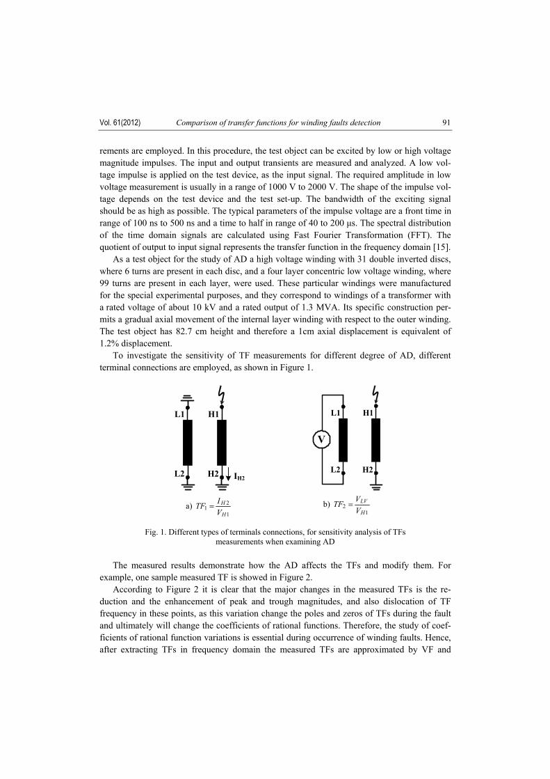
rements are employed. In this procedure, the test object can be excited by low or high voltage magnitude impulses. The input and output transients are measured and analyzed. A low vol-tage impulse is applied on the test device, as the input signal. The required amplitude in low voltage measurement is usually in a range of 1000 V to 2000 V. The shape of the impulse vol-tage depends on the test device and the test set-up. The bandwidth of the exciting signal should be as high as possible. The typical parameters of the impulse voltage are a front time in range of 100 ns to 500 ns and a time to half in range of 40 to 200 μs. The spectral distribution of the time domain signals are calculated using Fast Fourier Transformation (FFT). The quotient of output to input signal represents the transfer function in the frequency domain [15]. As a test object for the study of AD a high voltage winding with 31 double inverted discs, where 6 turns are present in each disc, and a four layer concentric low voltage winding, where 99 turns are present in each layer, were used. These particular windings were manufactured for the special experimental purposes, and they correspond to windings of a transformer with a rated voltage of about 10 kV and a rated output of 1.3 MVA. Its specific construction per-mits a gradual axial movement of the internal layer winding with respect to the outer winding. The test object has 82.7 cm height and therefore a 1cm axial displacement is equivalent of 1.2% displacement. To investigate the sensitivity of TF measurements for different degree of AD, different terminal connections are employed, as shown in Figure 1.

L2

L1

H2

H1

IH2

L2

L1

H2

H1

V

a) 1

21

H

H

VITF = b)

12

H

LV

VVTF =

Fig. 1. Different types of terminals connections, for sensitivity analysis of TFs measurements when examining AD

The measured results demonstrate how the AD affects the TFs and modify them. For example, one sample measured TF is showed in Figure 2. According to Figure 2 it is clear that the major changes in the measured TFs is the re-duction and the enhancement of peak and trough magnitudes, and also dislocation of TF frequency in these points, as this variation change the poles and zeros of TFs during the fault and ultimately will change the coefficients of rational functions. Therefore, the study of coef-ficients of rational function variations is essential during occurrence of winding faults. Hence, after extracting TFs in frequency domain the measured TFs are approximated by VF and


DPIF. In Figure 3 the results of approximations of TF1 is given for the intact winding using both VF and DPIF methods. Since the measured TF2 is the ratio of one voltage to another voltage, therefore the DPIF method is not identifiable and the TF approximation results, only using the VF method, is given in Figure 4.

0 0.1 0.2 0.3 0.4 0.5 0.6 0.7 0.8 0.9 110-7

10-6

10-5

10-4

10-3

10-2

Frequency [MHz]

Mag

nitu

de [A

/V]

0cm Displacement1cm Displacement2cm Displacement3cm Displacement4cm Displacement5cm Displacement6cm Displacement7cm Displacement8cm Displacement

Fig. 2. The measured TF of transformer under various degree of AD (setup TF1)

0 0.1 0.2 0.3 0.4 0.5 0.6 0.7 0.8 0.9 110

-5

10-4

10-3

10-2

Frequency [MHz]

Mag

nitu

de [m

A/V

]

MeasuredEstimated using VFEstimated using DPIF

Fig. 3. Comparison of the approximated TF1 using VF and DPIF methods versus the measurement

in intact case As shown in Figure 3, the TF approximation using both methods has led to good results but the accuracy of VF method is more than DPIF method. However to determine the fault


level from the measured TF, the magnitude and the frequency at the peak and trough points should be employed. Figure 3 shows how DPIF method is able to estimate these points. Low accuracy of DPIF method is due to its limitation in predicting very small oscillations of TFs that they have not an important role in fault detection.

0 0.1 0.2 0.3 0.4 0.5 0.6 0.7 0.8 0.9 110

-3

10-2

10-1

100

101

Frequency [MHz]

Mag

nitu

de [V

/V]

Measured

Estimated using VF

Fig. 4. Comparison of the approximated TF2 using VF method versus the measurement in intact case

5. Proposed method Tables 1 and 2 present sample results of estimated TFs in frequency domain using the VF and DPIF methods for the TF1 in intact case and degree 1 (1cm) of the AD, respectively. These results show that by the AD of the winding, the numerator and denominator coefficients of TFs change.

Table 1. Some of the selected numerator and denominator coefficients derived from the estimated TF1 using VF method

Numerator Denominator Order

intact case 1 cm displacement intact case 1 cm displacement s20 0 0 1 1 s19 !8.726e-5 !9.612e-5 4.7856 4.6754 s14 !3.1076 !3.0338 1.2107e5 1.2057e5 s8 !1346 !1309.2 3.8107e7 3.7857e7 s7 425.15 359.64 1.0878e8 1.0634e8 s2 9731.3 9527.7 5.6865e6 5.5665e6 s1 292.96 286.57 1.8288e5 1.7904e5 s0 1.928 1.8868 1633.5 1599.6


Table 2. Some of the selected numerator and denominator coefficients derived from the estimated TF1 using DPIF method

Numerator Denominator Order intact case 1 cm displacement intact case 1 cm displacement

s16 0 0 1 1 s15 0.001 0.001 1.5824 1.6674 s11 3.1637 3.1347 4559.3 4774.8 s10 10.529 10.274 79517 78951 s3 1435.2 1408.1 1.4554e6 1.4355e6 s2 959.58 943.78 2.38e6 2.3536e6 s1 490.38 484.8 3.8138e5 3.7717e5 s0 27.599 27.302 18060 17860

Therefore, to compare the TFs in winding intact form and its fault conditions, the follow-ing criterion can be offered:

,1∑=

−=

m

i if

inif

aaa

α (17)

where α is the sum of absolute differences of numerator coefficients, m is the number of nu-merator coefficients, fia and nia are the values of i-th coefficient for faulted and normal con-ditions, respectively. The β index can be defined by the same formulation to comparison of denominator coef-ficients as follow:

.1∑=

−=

n

i if

inif

bbb

β (18)

Using Equations (17) and (18) the measured TFs are compared, that the results of cal-culations is given in Table 3 for TF1. Because of the DPIF method is not able to identify the TF2, so the results are shown in Table 4 just using of VF method for TF2. Study of Tables 3 and 4 represent that the proposed indices as well have been able to detect the fault level with high accuracy. The β increases in both of VF and DPIF methods by increasing the level of fault regularly while the increase in α at VF method is not very suit-able. The results of this tables show that the both of methods are useful in winding fault detec-tion studies. Even in TF2 that rate of the TF changes is not too much, the VF method is well able to detect the fault level. In order to compare these two methods in a best way, and to prove the capabilities of the proposed indices, the rate of change is calculated using the definition of the change factor (CF), (for these indices) at each level, as follows:

.%100)(

)()1(×

−+=

iindexiindexiindexCF (19)

That CF represents the rate of change of proposed indices in i-th level of calculation.


Table 3. The calculations results of α and β using VF and DPIF methods (setup TF1)

α β Displacement (cm)

VF DPIF VF DPIF 1 1.2640 0.2606 0.3067 0.3297 2 3.8181 0.3829 1.2430 0.6979 3 6.5553 0.9862 2.4274 0.9847 4 8.5782 1.0786 3.4906 1.4252 5 9.7624 1.1523 4.3364 1.8083 6 10.9272 1.2320 5.3275 2.2403 7 11.6307 1.4330 5.8600 2.3425 8 11.8298 1.5653 6.3629 2.5451

Table 4. The calculations results of α and β using VF and DPIF methods (setup TF2)

Displacement (cm) α β

1 0.2609 0.2397 2 0.5456 0.4809 3 1.6987 1.6079 4 3.0453 2.9440 5 4.2031 4.0602 6 5.6333 5.1602 7 8.2901 7.1791 8 11.5446 10.3230

Table 5. The calculations results of CF

α β

VF VF Displacement (cm)

TF1 TF2 DPIF

TF1 TF2 DPIF

1 – – – – – – 2 202% 109% 46.9% 305% 100% 111% 3 71.6% 211% 157% 95.3% 234% 41.1% 4 30.8% 79.2% 9.3% 43.7% 83.1% 44.7% 5 13.8% 38.1% 6.8% 19.5% 37.9% 26.8% 6 11.9% 25.4% 6.9% 22.8% 27.1% 23.8% 7 6.4% 47% 16.3% 9.9% 20.2% 4.5% 8 1.7% 39.2% 9.2% 8.6% 43.8% 8.6%

Table 5 represents the calculation results of CF for the measured TFs. This table shows how employing the proposed indices, different fault levels are distinguished and the winding


fault levels are determined with a high accuracy. However, as it is mentioned above, α should only be used when the DPIF method is used to estimate the TFs, because according to Table 5 the amount of CF for ,α when using VF method and at the 8cm of displacement is the negligible 1.7%. In this case, the two AD of levels 7 and 8 can not be distinguished.

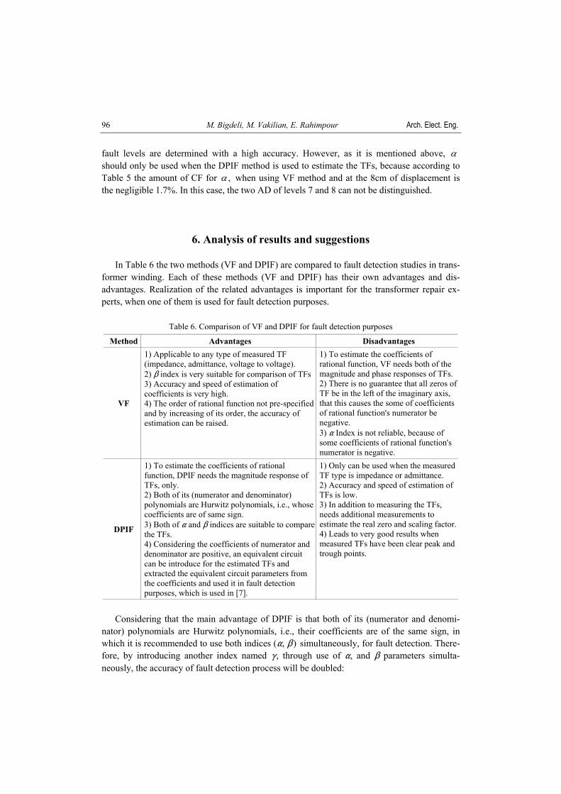
6. Analysis of results and suggestions In Table 6 the two methods (VF and DPIF) are compared to fault detection studies in trans-former winding. Each of these methods (VF and DPIF) has their own advantages and dis-advantages. Realization of the related advantages is important for the transformer repair ex-perts, when one of them is used for fault detection purposes.

Table 6. Comparison of VF and DPIF for fault detection purposes

Method Advantages Disadvantages

VF

1) Applicable to any type of measured TF (impedance, admittance, voltage to voltage). 2) $ index is very suitable for comparison of TFs 3) Accuracy and speed of estimation of coefficients is very high. 4) The order of rational function not pre-specified and by increasing of its order, the accuracy of estimation can be raised.

1) To estimate the coefficients of rational function, VF needs both of the magnitude and phase responses of TFs. 2) There is no guarantee that all zeros of TF be in the left of the imaginary axis, that this causes the some of coefficients of rational function's numerator be negative. 3) " Index is not reliable, because of some coefficients of rational function's numerator is negative.

DPIF

1) To estimate the coefficients of rational function, DPIF needs the magnitude response of TFs, only. 2) Both of its (numerator and denominator) polynomials are Hurwitz polynomials, i.e., whose coefficients are of same sign. 3) Both of " and $ indices are suitable to compare the TFs. 4) Considering the coefficients of numerator and denominator are positive, an equivalent circuit can be introduce for the estimated TFs and extracted the equivalent circuit parameters from the coefficients and used it in fault detection purposes, which is used in [7].

1) Only can be used when the measured TF type is impedance or admittance. 2) Accuracy and speed of estimation of TFs is low. 3) In addition to measuring the TFs, needs additional measurements to estimate the real zero and scaling factor. 4) Leads to very good results when measured TFs have been clear peak and trough points.

Considering that the main advantage of DPIF is that both of its (numerator and denomi-nator) polynomials are Hurwitz polynomials, i.e., their coefficients are of the same sign, in which it is recommended to use both indices (", $) simultaneously, for fault detection. There-fore, by introducing another index named (, through use of ", and $ parameters simulta-neously, the accuracy of fault detection process will be doubled:


...11

⎟⎟⎠

⎞⎜⎜⎝

⎛ −⎟⎟⎠

⎞⎜⎜⎝

⎛ −== ∑∑

==

n

i fi

nifim

i fi

nifi

bbb

aaa

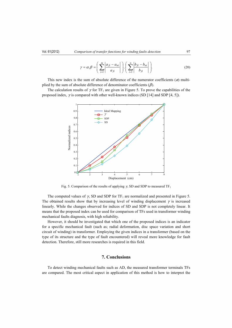
βαγ (20)

This new index is the sum of absolute difference of the numerator coefficients (") multi-plied by the sum of absolute difference of denominator coefficients ($). The calculation results of ( for TF1 are given in Figure 5. To prove the capabilities of the proposed index, ( is compared with other well-known indices (SD [14] and SDP [4, 5]).

1 2 3 4 5 6 7 80

0.1

0.2

0.3

0.4

0.5

0.6

0.7

0.8

0.9

1

Displacement (cm)

Nor

mal

ized

indi

ces

Ideal Mapping

SDPSD

γ

Fig. 5. Comparison of the results of applying (, SD and SDP to measured TF1 The computed values of (, SD and SDP for TF1 are normalized and presented in Figure 5. The obtained results show that by increasing level of winding displacement ( is increased linearly. While the changes observed for indices of SD and SDP is not completely linear. It means that the proposed index can be used for comparison of TFs used in transformer winding mechanical faults diagnosis, with high reliability. However, it should be investigated that which one of the proposed indices is an indicator for a specific mechanical fault (such as; radial deformation, disc space variation and short circuit of winding) in transformer. Employing the given indices in a transformer (based on the type of its structure and the type of fault encountered) will reveal more knowledge for fault detection. Therefore, still more researches is required in this field.

7. Conclusions To detect winding mechanical faults such as AD, the measured transformer terminals TFs are compared. The most critical aspect in application of this method is how to interpret the


measured TFs and how to compare them. In this paper the rational function coefficients are compared, for comparison of TFs. To estimate the coefficients of the rational function, two ro-bust and reliable estimation methods (VF and DPIF) are introduced in the frequency domain. Introducing two new indices (", $) , based on the coefficients of numerator and denominator of rational function, the measured TFs are compared. Moreover, comparison is made between VF and DPIF methods for fault detection studies. The obtained results indicate that: 1) The $ index when using one of the VF or the DPIF methods, correctly determines the fault

level, 2) Due to the existence of a negative value for some rational function numerator coefficients

in VF method, the " index would not provide reliable results for this method. While, this index in DPIF method has led to reliable results,

3) Another index (() based on simultaneous use of coefficients of numerator and denomi-nator of rational function is introduced which is more reliable than the previous indices.

Depending on the kind of TF which is available, and also the required accuracy and speed, each one of the proposed indices can be used. References [1] Singh A., Castellanos F., Marti J.R., Srivastava K.D., A Comparison of Trans-Admittance and Cha-

racteristic Impedance as Metrics for Detection of Winding Displacements in Power Transformers. Electric Power Systems Research, Elsevier 79: 871-877 (2009).

[2] Gustavsen B., Semlyen A., Rational Approximation of Frequency Domain Responses by Vector Fit-ting. IEEE Transactions on Power Delivery 14: 1052-1061 (1999).

[3] Gustavsen B., Wide Band Modeling of Power Transformers. IEEE Transactions on Power Delivery 19: 414-422 (2004).

[4] Karimifard P., Gharehpetian G.B., Tenbohlen S., Determination of Axial Displacement Extent Based on Transformer Winding Transfer Function Estimation using Vector-Fitting Method. European Transactions on Electrical Power 18: 423-436 (2008).

[5] Karimifard P., Gharehpetian G.B., Tenbohlen S., Localization of Winding Radial Deformation and Determination of Deformation Extent Using Vector Fitting-Based Estimated Transfer Function. European Transactions on Electrical Power 19: 749-762 (2009).

[6] Ragavan K., Satish L., Construction of Physically Realizable Driving-Point Function From Measured Frequency Response Data on a Model Winding. IEEE Transactions on Power Delivery 23: 760-767 (2008).

[7] Ragavan K., Satish L., Localization of Changes in a Model Winding Based on Terminal Measure-ments: Experimental Study. IEEE Transactions on Power Delivery 22: 1557-1565 (2007).

[8] Nirgude P.M., Ashokraju D., Rajkumar A.D., Singh B.P., Application of Numerical Evaluation Techniques for Interpreting Frequency Response Measurements in Power Transformers. IET Science, Measurements and Technology 2: 275-285 (2008).

[9] Leibfried T., Feser K., Monitoring of Power Transformers using the Transfer Function Method. IEEE Transactions on Power Delivery 14: 1333-1341 (1999).

[10]Christian J., Feser K., Procedures for Detecting Winding Displacements in Power Transformers by the Transfer Function Methods. IEEE Transactions on Power Delivery 19: 214-220 (2004).

[11]Ryder S.A., Diagnosing Transformer Faults using Frequency Response Analysis. IEEE Electrical Insulation Magazine 19: 16-22 (2003).

[12]Secue J.R., Mombello E., Sweep Frequency Response Analysis (SFRA) for the Assessment of Winding Displacements and Deformation in Power Transformers. Electric Power Systems Research, Elsevier 78: 1119-1128 (2008).


[13] Bigdeli M., Vakilian M., Rahimpour E., A New Method for Detection and Evaluation of Winding Mechanical Faults in Transformer through Transfer Function Measurements. Advances in Elec-trical and Computer Engineering 11: 23-30 (2011).

[14]Karimifard P., Gharehpetian G.B., A New Algorithm for Localization of Radial Deformation and Determination of Deformation Extent in Transformer Windings. Electric Power Systems Research, Elsevier 78: 1701-1711 (2008).

[15]Rahimpour E., Christian J., Feser K., Mohseni H., Transfer Function Method to Diagnose Axial Dis-placement and Radial Deformation of Transformer Winding. IEEE Transactions on Power Delivery 18: 493-505 (2003).

Date post:	08-Feb-2022
Category:	Documents
Upload:	others
View:	4 times
Download:	0 times

Comparison of transfer functions using estimated rational ...

Documents