Pages: 75 Characters: 145000

Comparison of Value-at-Risk Estimates from

GARCH Models

Supervisor: Jens Borges

J

Fannar Jens Ragnarsson

Master’s Thesis

Department of Economics Master of Science in Applied Economics & Finance

November 2011

Acknowledgements First of all I would like to thank CBS for offering the masters line Applied Economics &

Finance, I enjoyed the courses it offered and found the subjects very compelling and

intriguing. I would also like to thank the Department of Economics for all the help. Jens

Borges, my supervisor for giving me great recommendations on how this project should be

formulated. My dear friend Davíð Steinar Guðjónsson for helping me reviewing the project

and managing to dig into my computer and find a recent back up file when Microsoft Word

decided to change all that was written into symbols. Also I would like to thank his family for

providing me with great office space to work in.

Last but not least I would like to thank my family and friends for their endless support during

the whole process.

Executive Summary This thesis has the objective to compare Value-at-Risk estimates from selected GARCH

models. It will start with a theoretical part which familiarizes the reader with Value-at-Risk

and its main concepts. Known models will be explained and applied, time-series analysis with

theories and tests for financial time-series are discussed. For evaluating different Value-at-

Risk estimates backtests will be described and discussed.

The empirical part of this research starts with the selection process for the preferred GARCH

(p, q) model, on the time-series of S&P500 Total Return index ranging from 20.07.01-

19.07.11 (10 years of data).

The selected model is a restricted GARCH (1, 2) model which is evaluated against the

GARCH (1, 1) model and the Riskmetrics model. These models were evaluated at the 5% and

1% Value-at-Risk levels for three sample periods. One being the Full sample, another the

Before Crisis sample and lastly the With Crisis sample.

The results of the evaluations for the models showed that it is hard to select one of them, as

the best model for the time-series. The GARCH (1, 1) performed best on the Full sample,

while the Riskmetrics performed best on the Before Crisis sample and the GARCH (1, 2)

performed best on the With Crisis sample.

i

Table of Contents

1   Introduction .......................................................................................................................... 1  

1.1   Objective ....................................................................................................................... 1  

1.2   Methodology & Delimitations ...................................................................................... 2  

2   Value-at-Risk ....................................................................................................................... 3  

2.1   Development ................................................................................................................. 3  

2.2   Fundamentals ................................................................................................................ 4  

2.2.1   Mark to Market ....................................................................................................... 4  

2.2.2   Holding Period ....................................................................................................... 5  

2.2.3   Observation Period ................................................................................................. 5  

2.2.4   Confidence Level ................................................................................................... 6  

2.2.5   CESR Regulation for UCITS ................................................................................. 8  

2.2.6   BASEL Regulation ................................................................................................. 9  

2.3   Popular Methods ........................................................................................................... 9  

2.3.1   Historical Simulation .............................................................................................. 9  

2.3.2   Variance Covariance ............................................................................................ 11  

2.3.3   Monte Carlo Simulation ....................................................................................... 12  

2.3.4   Riskmetrics ........................................................................................................... 14  

3   Time-Series Analysis ......................................................................................................... 16  

3.1   Iterated Cumulative Sums of Squares (ICSS) Algorithm ........................................... 21  

3.2   Autoregressive Conditional Heteroskedasticity (ARCH) ........................................... 24  

3.3   Generalized Autoregressive Conditional Heteroskedasticity (GARCH) .................... 26  

4   Backtests ............................................................................................................................. 28  

4.1   Basel Traffic Light Approach ..................................................................................... 28  

4.2   Kupiec Test ................................................................................................................. 29  

4.3   Christoffersen Test ...................................................................................................... 30  

4.4   Test for Conditional Coverage .................................................................................... 31  

4.5   Pearson’s Q Test .......................................................................................................... 31  

4.6   Lopez’s Loss Function ................................................................................................ 32  

5   Empirical Research ............................................................................................................ 33  

ii

5.1   Model Selection Process ............................................................................................. 33  

5.2   Ljung-Box Q Test ........................................................................................................ 38  

5.3   ARCH Test .................................................................................................................. 39  

5.4   Parameter Estimation .................................................................................................. 41  

5.5   Backtest Samples ......................................................................................................... 42  

5.6   Backtest Results .......................................................................................................... 44  

5.6.1   Full ....................................................................................................................... 45  

5.6.2   Before Crisis ......................................................................................................... 46  

5.6.3   With Crisis ............................................................................................................ 48  

5.6.4   Lopez’s Loss Function ......................................................................................... 50  

5.6.4.1   Violation Exceedance for Rolling GARCH (1, 1) ........................................ 51  

5.6.4.2   Violation Exceedance for Rolling Restricted GARCH (1, 2) ....................... 53  

5.6.4.3   Violation Exceedance for Riskmetrics .......................................................... 55  

6   Discussion .......................................................................................................................... 57  

7   Conclusion .......................................................................................................................... 59  

8   Bibliography ....................................................................................................................... 61  

9   Appendix A: VBA Codes ................................................................................................... 63  

9.1   ICSS Algorithm ........................................................................................................... 63  

9.2   Nelder-Mead Algorithm .............................................................................................. 69  

9.3   Variance Forecasts ...................................................................................................... 74  

iii

Table of Figures

Figure 1: Normal distribution and confidence levels for Value-at-Risk .................................... 7  

Figure 2: Histogram of daily returns, S&P500 TR index (20.7.10-19.7.11) ........................... 10  

Figure 3: Histogram & normal distr. of daily returns, S&P500 TR index (20.7.10-19.7.11) .. 11  

Figure 4: Histogram of returns by Monte Carlo, S&P500 TR index (20.7.10-19.7.11) .......... 13  

Figure 5: Graph showing how different lambda values affect sample weights ....................... 15  

Figure 6: Line graph displaying daily returns, S&P500 TR index (20.7.1-19.7.11) ................ 17  

Figure 7: Correlogram for daily returns, S&P500 TR index (20.7.1-19.7.11) ......................... 18  

Figure 8: Correlogram of squared daily returns, S&P500 TR index (20.7.1-19.7.11) ............ 20  

Figure 9: Daily returns and ICSS change points, S&P500 TR index (20.7.1-19.7.11) ........... 23  

Figure 10: Sample ranges used for baktesting, S&P500 TR index (20.7.1-19.7.11) ............... 43  

Figure 11: Size and distribution of violations (5% VaR), rolling GARCH (1, 1) ................... 51  

Figure 12: Size and distribution of violations (1% VaR), rolling GARCH (1, 1) ................... 51  

Figure 13: Size and distribution of violations (5% VaR), rolling restricted GARCH (1, 2) .... 53  

Figure 14: Size and distribution of violations (1% VaR), rolling restricted GARCH (1, 2) .... 53  

Figure 15: Size and distribution of violations (5% VaR), Riskmetrics .................................... 55  

Figure 16: Size and distribution of violations (1% VaR), Riskmetrics .................................... 55  

iv

List of Tables

Table 1: Ljung-Box Q test for daily returns, S&P500 TR index (20.7.1-19.7.11) .................. 19  

Table 2: AIC and SBC statistics for various GARCH models ................................................. 34  

Table 3: Estimated parameters for the GARCH (1, 2) model .................................................. 35  

Table 4: Estimated parameters for the GARCH (1, 1) model .................................................. 36  

Table 5: Estimated parameters for the restricted GARCH (1, 2) model .................................. 37  

Table 6: Ljung-Box Q test for the GARCH (1, 1) model ........................................................ 39  

Table 7: Ljung-Box Q test for the restricted GARCH (1, 2) model ......................................... 39  

Table 8: ARCH test for the GARCH (1, 1) model ................................................................... 40  

Table 9: ARCH test for the restricted GARCH (1, 2) model ................................................... 41  

Table 10: Backtest results for the Full sample ......................................................................... 45  

Table 11: Backtest results for the Before Crisis sample .......................................................... 46  

Table 12: Backtest results for the With Crisis sample ............................................................. 48  

Table 13: Lopez’s loss function results for the Full sample .................................................... 50  

1

1 Introduction

With financial markets being abnormally turbulent in recent years, the task for financial firms

to manage risk is even more compelling. One of the main factors of managing financial risk is

the calculation of Value-at-Risk. This project explains the concept of Value-at-Risk. The

development of Value-at-Risk will be briefly discussed and the fundamentals of the concept.

They need to be considered carefully before applying a Value-at-Risk model to a portfolio,

despite which model is chosen. Four of the most well known models will be shown, described

and applied to the S&P500 Total Return index, which will be used throughout this paper for

application and evaluation of Value-at-Risk models.

Statistical analysis of financial time-series will be shown in this paper since it is important to

know the common behavior of financial time-series while working with them.

For Value-at-Risk it is not enough to simply choose a model and apply it on the portfolio at

hand. One needs to evaluate the model and preferably compare its performance to other

models. Since one model might fit well to certain time-series, but fail when it is applied to a

different set of time- series. The evaluation process for Value-at-Risk estimations is called

backtesting, the methods for it will be described and applied.

The empirical research will consist of analysis on the time-series for the S&P500 Total

Return index with data ranging back ten years, selecting Value-at-Risk models to apply on the

time-series and then compare them.

1.1 Objective This thesis contributes to empirical studies, familiarizes the reader with the fundamental

concepts and backtests of Value-at-Risk and the theories behind them. The empirical research

is where Generalized Autoregressive Conditional Heteroskedasticity (GARCH) models will

be applied to time-series, they compared to each other and a chosen benchmark model. The

main objective is to see which of these models predicts Value-at-Risk most accurately on the

past ten years of the S&P500 Total Return index.

1.2 METHODOLOGY & DELIMITATIONS CHAPTER 1. INTRODUCTION

2

1.2 Methodology & Delimitations The theories that will be applied in this study will be done by the use of Microsoft Excel, with

the help of Visual Basic Application (VBA), for computations that Excel’s built in functions

cannot easily handle. In some cases computations will be executed in MATLAB a well

known mathematical and statistical software. It should be noted that a lot of time was spent on

writing, debugging and running the VBA codes, and the worksheets attached to the enclosed

CD.

Although Value-at-Risk is sometimes referred to as a measurement for normal market

behaviours, since it does very seldom manage to mitigate risks during abnormal market

behaviours, the financial crisis of late 2008 will be covered in the research.

Furthermore the model selection process for this thesis will try to find the best model from the

GARCH (p, q) models, hybrids or extensions from this model will not be considered

Since there are many statistical tests discussed and applied in this paper, it should be noted

that there is always a possibility of type I or type II errors with hypothesis tests. A type I error

is when a test rejects a true null-hypothesis and a type II error is when a test fails to reject a

false null hypothesis.

With relation to the mathematics and statistics, proofs for functions and formulae presented

will not be shown, it is beyond the scope of this thesis.

The assumption for normality will hold throughout this paper.

.

3

2 Value-at-Risk

“Risk is like fire: if controlled it will help you, if uncontrolled it will rise up and destroy you.”

Theodore Roosevelt

Value-at-Risk is a measure of the risk an entity is facing by its operations. A number that

states how much can be lost after a period of time. This number is derived from calculations

made by e.g. the risk manager who is trying to get a glimpse into the magnitude of potential

losses of the current position. While constructing Value-at-Risk selecting the method used for

the calculation is of upmost importance. This can lead to a strong number if done properly

and if not much thought is put into the selection process of a method it is more likely to lead

to a weaker Value-at-Risk estimate.

In this chapter the development of Value-at-Risk, fundamentals and some of the most known

methods will be discussed.

2.1 Development During the late 1970s and 1980s many major financial institutions began working on models

that were designed to measure and aggregate risks throughout their whole operations. At this

time there was a high demand for such models since there had been a fair amount of financial

crisis right before and during this timespan. The most well known of these and still popular

today is the Riskmetrics system, which was introduced by JP Morgan. It is said that the

manager of JP Morgan, Dennis Weatherstone, asked his staff to write a daily one page report

that would account for risks and potential losses over the next 24 hours, for the banks total

trading portfolio. The staff at JP Morgan then developed a risk measurement that shows the

maximum likely loss over the next trading day in one number, it was called Value at Risk

(Dowd, 1998).

Value-at-Risk was derived from the breakthrough research that Harry Markowitz made on

portfolio theory in the 1950s. He later received the Nobel Memorial Prize in Economic

Sciences for his contribution. Markowitz’s research confirmed that the standard deviations

and expected returns of portfolios could be estimated within the framework of the normal

distribution and could tell a story about the risk involved. While smaller standard deviation

exhibits less risk but consequently often reduces the expected return, making a trade-off

2.2 FUNDAMENTALS CHAPTER 2. VALUE-AT-RISK

4

between risk and return. Markowitz’s research motivated portfolio managers to diversify their

portfolios and calculate correlations, standard deviations and expected returns between

securities within their current position (Jorion, 2007).

When the staff at JP Morgan tried to solve the problem they concentrated on the left or

negative side of the normal distribution while they constructed Value-at-Risk. In October

1994 JP Morgan decided to make the Riskmetrics system public. This lead many small

software providers to include it in new software packages or implement it in its existing

software, numerous financial institutions made use of it (Dowd, 1998).

There have been many other methods developed and few will be included in later sections,

however JP Morgan’s Riskmetrics seems to be a good benchmark for evaluating other models

and will be used as such for the purpose of this research.

2.2 Fundamentals There are three parameters that always have to be kept in mind and stated when Value-at-Risk

is computed, these parameters are more of a specification for the Value-at-Risk. They will be

described in sections 2.2.2-2.2.4 and sections 2.2.5-2.2.6 will describe how the regulators

want these specifications to be. The first section will explain why it is important to use market

values when calculating Value-at-Risk.

2.2.1 Mark to Market One of the crucial parts of risk management is to mark to market. That means that they need

to think about daily market changes instead of using accrual accounting methods. They

observe how securities rise or fall instead of waiting until they materialize. With accrual

methods losses were often revealed only when securities maturated. If they would not have

waited and the security had lost value, they could have acted earlier and prevented further loss.

Also when marking to market the investor can see volatilities and take account for them

(Dowd, 1998).

In this research the assumption will be made that the investor reinvests all dividends allocated

in the portfolio and therefore it will consist of the S&P500 Total Return index instead of the

normal S&P index, since the Total Return index adjusts the index rate for dividends. An

2.2 FUNDAMENTALS CHAPTER 2. VALUE-AT-RISK

5

investor that compares his portfolio profits to a market portfolio that is not adjusted to

dividends could think that he has beaten the market, where he really has not, since he has

benefitted from dividend payments.

2.2.2 Holding Period Usually the holding period is chosen to be one day or one month, but there can be varieties in

holding periods based on the type of portfolio. The main factors that affect the choice of

holding period are four. First is the liquidity of the portfolio, if it is in a market that has very

frequent trading, shorter holding period would be efficient, because then it is easy to get rid of

assets in the portfolio or exchange assets almost instantly. However if it is hard to get

counterparty for trades in the market, like in many Over The Counter (OTC) markets a longer

holding period is usually chosen since the market is less liquid.

The other three factors all suggest shorter holding periods, one of them is for the normal

approximation to be more efficient, with a short holding period the normal approximation

usually makes a better fit to the position. Another reason is to adjust for changes in the

portfolio. If the chosen holding period is one month a manager would want to change his

position if it is showing losses, but with a one day holding period changes in exposures can be

made more frequently and therefore reduce the risk of an unwanted loss.

Shorter holding periods are better for valuation purposes, for example with one day holding

period it does not take a long time until the sample that is forecasted from is large enough,

with one year giving around 250 observations. However with a holding period of one month it

would take almost 21 years to get 250 observations and since the first observation would have

happened more than two decades ago, changes in the macro environment (politics, technology,

currencies etc.) are likely to make the observation obsolete (Dowd, 1998).

2.2.3 Observation Period The choice of observation period is important, it depends on which model is being used, for

the Riskmetrics model which will be explained in section 2.3.4, the observation period does

not matter as long as enough observations are included for all the related weights to have an

impact on the outcome. However with models such as the Variance Covariance model or the

2.2 FUNDAMENTALS CHAPTER 2. VALUE-AT-RISK

6

Historical Simulation model (explained in section 2.3.1) the observation period is of high

importance, since all observations are given equal weight. The observation period simply

specifies what range of previous observations should be used when calculating the Value-at-

Risk number. So an observation period of 250 would use the last 250 observations to obtain

Value-at-Risk.

2.2.4 Confidence Level The confidence level explains how often the observed results or portfolio returns should

exceed the Value-at-Risk number. Usually confidence levels ranging from 90% to 99% are

used and most often 95% or 99%. For the 99% confidence level you would expect the

observed loss to exceed the forecasted Value-at-Risk number once every hundred

observations. For evaluation purposes the 95% confidence level is more convenient because

exceedance from the forecasted Value-at-Risk number should happen more frequently.

Institutions use Value-at-Risk to specify capital requirements, then a risk averse institution

would prefer to set the confidence level at higher rate, closer to or even exceeding the 99%

level. Since then the capital requirements would be higher and less risk of not being able to

cover losses in its exposures. Figure 1 shows how different confidence levels are calculated if

the normality assumption is used.

2.2 FUNDAMENTALS CHAPTER 2. VALUE-AT-RISK

7

Figure 1: Normal distribution and confidence levels for Value-at-Riski

One of the conveniences from using the normal assumption is that it is very easy to construct

Value-at-Risk at different confidence levels. For example if a bank wants to compare its

Value-at-Risk number to another bank, but they do not publish their Value-at-Risk numbers at

the same confidence level. It can simply adjust the number to whatever confidence level it

chooses to, in order for that to work the normality assumption must be used in both cases.

Confidence level 99% 95%

Value-at-Risk ! − 2,326  ×  ! ! − 1,645  ×  !

As seen above the only variables needed are the mean, standard deviation and the confidence

level, the numbers 2,326 and 1,645 are the coefficients for the 99% and 95% confidence

levels respectively. After the confidence level has been chosen and Value-at-Risk achieved

the whole value of the underlying portfolio is multiplied by the Value-at-Risk number to see

how much it is in the given currency. When financial institutions make the normality

assumption they sometimes make the assumption as N (0,  !!) the mean returns are assumed

to be zero. It can be debated if the assumption for zero mean should be used, but the mean for

daily observations is usually a little bit above zero. For the risk manager using a holding

period of daily returns the assumption of zero mean can be justified. As for longer horizons, it

would not be wise to make the zero mean assumption (Dowd, 1998).

i This graph can be found in the Excel worksheet normaldistributiongraph.xlsm on the enclosed CD.

2.2 FUNDAMENTALS CHAPTER 2. VALUE-AT-RISK

8

Being a convenient way for Value-at-Risk forecasting, the normal assumption has its pitfalls.

One of them is that securities tend to have fatter tails than accounted for by the normal

distribution. Meaning that Value-at-Risk models using the normal assumption might

underestimate the Value-at-Risk. Other approaches have been used such as changing the

distribution to e.g. the Student-T, which can account for fatter tails or by using the Historical

Simulation method, which does not assume for any kind of distribution (Dowd, 1998).

2.2.5 CESR Regulation for UCITS The Committee of European Securities Regulators (CESR) have directives for Undertakings

for the Collective Investment in Transferable Securities (UCITS), those directives account for

funds that are operating in countries within the European Union. There are also domestic

regulations, which are different from country to country within the EU, but CESR regulations

are used as a base point.

With regards to the publication of Value-at-Risk for funds that are specified as UCITS the

base regulation enforces the calculation of Value-at-Risk and specifies what the maximum

Value-at-Risk value should be, it is stated that it should never surpass 20% when the

parameters discussed earlier in this section are at a predefined value. According to CESR

guidelines set in July 2010 the confidence level should be set at 99%, holding period equal to

one month (20 business days) and observation period at least one year (250 business days)

unless external factors suggest a shorter period e.g. for a drastic change in price volatilities

during an extreme market condition. As mentioned in this section, to have a holding period of

a month can be troublesome since observations might be too few. That is why CESR have

allowed for rescaling of the Value-at-Risk number, if UCITS are using 95% confidence level,

they can rescale it according to the normal distribution. Also if they are using a holding period

of less than 20 business days they are allowed to rescale the Value-at-Risk number using the

square root of time rule. This rule can be shown as follows:

!"#   !  !"#$ ≈  !!  ×  !"#(!  !"#$)

If it is needed to rescale a daily horizon up to 20 days as CESR sets for the maximum Value-

at-Risk, x is simply set to a value of 20 while t is set to a value of 1 (Committee of European

Securities Regulators, 2010).

2.3 POPULAR METHODS CHAPTER 2. VALUE-AT-RISK

9

2.2.6 BASEL Regulation The Basel Committee on Banking Supervision (BCBS) set guidelines and standards for banks

so that minimum requirements of BCBS are met.

Basel sets minimum requirements for quantitative standards of Value-at-Risk for banks in

their revision to the Basel II market risk framework. It states that Value-at-Risk must be

calculated on a daily basis, it must have a confidence level of 99% and the holding period set

at 10 days. The observation period should be a minimum of 250 days. The observation period

can be less than a year if unusual conditions are in the market increasing the price volatility.

As with the CESR guidelines this does not mean that banks should use exactly those

parameters when estimating Value-at-Risk for their internal risk management. They are also

allowed to rescale from e.g. the normal distribution and by using the square root of time rule

(Basel Committee on Banking Supervision, 2011).

2.3 Popular Methodsi In this section the models that are most popular or common in the literature and in practice

will be explained, the ones that are most often mentioned in discussions about Value-at-Risk

models are the Historical Simulation, Variance Covariance and Monte Carlo Simulation.

Those models can be described as the core models since many models have been created

based on one or more of these three. The Riskmetrics model will be explained as well, since it

will be used as a benchmark in this research.

2.3.1 Historical Simulation Historical Simulation ranks the losses and gains from the worst and upwards. For illustration

a Historical Simulation distribution will be shown for the S&P500 Total Return index. Figure

2 shows a frequency histogram for daily returns of the S&P500 Total Return index. The

darker bars in the histogram represent the worst 5% of daily returns.

i Computation of all the graphs presented in section 2.3 can be found in the Excel worksheet popularmethods.xlsm on the enclosed CD.

2.3 POPULAR METHODS CHAPTER 2. VALUE-AT-RISK

10

Figure 2: Histogram of daily returns, S&P500 TR index (20.7.10-19.7.11)

In order to find the Value-at-Risk based on the Historical Simulation the observations should

first be ranked from worst to best, then use the number as Value-at-Risk that corresponds to

the percentile of the distribution based on the chosen confidence level. To calculate the 95%

Value-at-Risk for a one-year observation period of the S&P500 Total Return index, which

gives 253 observations, when the daily returns have been ranked the position of the 5th

percentile is found by multiplying 0,05 with the number of observations. In the case of the

S&P500 Total Return index sample used in Figure 2, that number is 12,65, so the 5% Value-

at-Risk (with a confidence level of 95%) is based on the 13th number out of the ranking order.

For the sample the 5% Value-at-Risk for the next day is 1.4626% so based on the Historical

Simulation there is a 5% chance of losing 1.4626% or more for this particular portfolio in the

next day.

Advantages of the Historical Simulation would be how easy it is to implement and explain to

others. It does not depend on any kind of assumption for the distribution of returns, therefore

it does not come with the problem of accounting for fat-tails of the distribution, as tends to

happen with the normal distribution. The Historical Simulation has disadvantages since it

bases its prediction on past returns. Each observation has an equal weight. An observation

that happened recently therefore has the same weight as an observation from a later period. A

left-tailed outlier will affect the results of the historical simulation until it is dropped out of

the window given by the observation period (Dowd, 1998).

2.3 POPULAR METHODS CHAPTER 2. VALUE-AT-RISK

11

2.3.2 Variance Covariance The Variance Covariance approach assumes for the normal distribution, few of its features

were explained in section 2.2.4. It simply approximates the returns from the observation

window to the normal distribution. The only parameters needed for the Variance Covariance

method are average returns and standard deviation of returns. The standard deviation is

multiplied by the confidence coefficient determined by the confidence level chosen. When

this approach is used on a portfolio the correlation and covariance between the assets in the

portfolio are calculated and from them the standard deviation is achieved. The following

formula shows how the portfolio variance is calculated.

!!! = !!!!!!!

+ !!!!!!"!!!!!!!!

Where ωi/j represents the weights of asset i or j and ρij represents the correlation coefficient

between the returns on assets i and j. The portfolio standard deviation is the square root of the

portfolio variance (Dowd, 1998). As with the Historical Simulation the Variance Covariance

method is used on the S&P Total Return index and the following graph shows the results.

Figure 3: Histogram & normal distr. of daily returns, S&P500 TR index (20.7.10-19.7.11)

2.3 POPULAR METHODS CHAPTER 2. VALUE-AT-RISK

12

The 5% Value-at-Risk is lower than the one from the Historical Simulation or at 1,3290%.

The frequency distribution is in Figure 3 to see if the actual distribution deviates from the

normal distribution. The frequency distribution does not seem too far away, although not fully

correlated with the normal distribution. The Jarque-Bera test for normality, checks if the

sample distribution has skewness and kurtosis that match the normal distribution. It is

asymptotically chi-square distributed and has two degrees of freedom, making the critical rate

5,99 at the 95% confidence level. The test statistic is calculated as follows:

!" =  !6 !! +

14 (! − 3)

!

Where JB represents the Jarque-Bera test statistic, n represents number of observations, S

represents skewness and K represents kurtosis (Jarque & Bera, 1980). The Jarque-Bera test

statistic on the one year sample for S&P500 Total Return index gave a value of 8,1201

rejecting the null hypothesis of normality at the 95% confidence level. The assumption could

not be rejected at the 99% confidence level since the critical value is lower than the observed

statistic.

Advantages of the Variance Covariance approach are how easy it is to implement and fetch

other important statistical details from the parameters it estimates. It can be troublesome to

explain this method to someone that has not been trained using the normal distribution and

therefore will not understand its core concepts. The assumption for the normal distribution

does not always represent the financial instruments it is modeling since those instruments

often tend to have fatter tails than the normal distribution accounts for (Dowd, 1998).

2.3.3 Monte Carlo Simulation The idea behind the Monte Carlo Simulation is to simulate random processes affecting the

prices of financial instruments. With each simulation predicting a value for the portfolio after

the chosen horizon period. For the Monte Carlo Simulation to be more efficient, a high

number of simulations are needed. If the amount of simulations is large enough the simulation

has converged to the portfolio’s “true” unknown distribution. At the beginning of the process

a model must be chosen and its parameters estimated. Then a hypothetical price path is

simulated that depends on the model and the random numbers generated (Dowd, 1998).

2.3 POPULAR METHODS CHAPTER 2. VALUE-AT-RISK

13

A Monte Carlo Simulation was run on the same observation period as with previous models.

This simulation is based on Geometric Brownian Motion, which has been widely used to

simulate stock prices. Price paths are simulated for the next day after the latest observation in

the sample. Parameters used in the simulation are estimates from the sample, the estimate for

the standard deviation and the mean. Then the representation of the time interval t is chosen,

in this simulation it represents a minute. There are 1440 minutes in a day resulting in 1440

random processes for each return forecast. The model is as follows:

!! = !!!!!!!!!!

! !!!!

Where P is the price of the asset, µ is the mean return and Wt is a geometric Wiener process,

which is a random number generated from the normal distribution. The mean and the standard

deviation need to be converted to the time interval, since the time interval is a minute in order

to acquire the correct parameters the daily mean from the sample is divided by 1440 and the

daily standard deviation is divided by the square root of 1440 (using the square root of time

rule). This model simply describes a random walk with a drift. The reason for subtracting half

the variance from the mean is to account for eroding returns (Croce, 2009). The simulation

was run 1000 times gaining 1000 different returns for the next day, it did not fully converge,

which will take a lot more simulations to achieve, but it is enough to show how the Monte

Carlo Simulation works. Figure 4 presents the frequency distribution of the obtained returns.

Figure 4: Histogram of returns by Monte Carlo, S&P500 TR index (20.7.10-19.7.11)

2.3 POPULAR METHODS CHAPTER 2. VALUE-AT-RISK

14

Since there were 1000 observations, in order to find the 5% Value-at-Risk based on the

Monte Carlo Simulation the resulting observations are sorted from lowest to highest and the

51st represents the 5% Value-at-Risk, for the Monte Carlo Simulation that number is 1,3114%.

Since the random process was based on the normal distribution the frequency distribution is

near normal, in fact the Jarque-Bera test statistic is 0,5295. It significantly accepts the

hypothesis for a normal distribution and with convergence the test statistic should be even

lower.

There are many advantages to the Monte Carlo Simulation since almost any model can be

used and simulated. One disadvantage is its time consuming nature i.e. it is computationally

intensive to generate all the simulations needed. Another disadvantage is how problematic it

is to describe to others, even more difficult than with the Variance Covariance approach.

2.3.4 Riskmetrics As with all models previously discussed (except for the Historical Simulation) the

Riskmetrics model measures volatility of the sample data. There is one added feature; it does

not give equal weights to all the observations within the sample period like the Variance

Covariance model. It uses Exponentially Weighted Moving Average (EWMA). Which adds a

decay factor to the model, it determines how the different weights are distributed among the

sample observations. JP Morgan set a value for the decay factor, being 0.94 for daily and 0.99

for monthly holding periods. Historical time-series of stock prices are known to show

volatility clustering, meaning that volatilities tend to cluster together, making periods with

high and low volatilities. The Riskmetrics model can be shown as follows:

!!! = !!!!! 1− ! + !  !!!!!

Where lambda represents the decay factor. Figure 5 shows how the weights change with

different lambda values.

2.3 POPULAR METHODS CHAPTER 2. VALUE-AT-RISK

15

Figure 5: Graph showing how different lambda values affect sample weights

The weights of each return diminishes exponentially over time, since the lambda value

controls the weights, it therefore decides the size of the observation window. The result from

calculating log (0.001)/log (λ) shows at which previous period the accumulated weights are

up to 99,9% of the variance calculated by the model. For a lambda value of 0.94 that number

would be 111,64 making the 112th observation as the latest to be included for 99,9% of the

weights. As with a lambda value of 0.97 that number would move up to 227 days   (Mina &

Xiao, 2001). The Riskmetrics method was applied to the S&P Total Return index (20.07.10-

19.07.11). It gave 1,5733% Value-at-Risk at the 5% level.

The Riskmetrics model is actually an IGARCH (1,1) process with no constant, GARCH

models will be discussed in the next section and the features of the Riskmetrics model help to

understand the different GARCH models.

From all the models, 5% Value-at-Risk was calculated with each giving different results.

16

3 Time-Series Analysis

All the models described in the previous section can be placed under the umbrella of time-

series analysis. For time-series analysis in the literature for econometric research the

Autoregressive Conditional Heteroskedasticity (ARCH) and Generalized Autoregressive

Conditional Heteroskedasticity (GARCH) models are frequently discussed. Robert Engle

pioneered the ARCH model in 1982 (which he in 2003 shared the Nobel Price in Economics

for) and in 1986 Tim Bollerslev introduced the GARCH model. The Riskmetrics model can

easily fit into that group as well, being a slightly modified version of the IGARCH (1, 1)

model.

ARCH and GARCH models measure volatility. They are based on least squares model, it

assumes that expected values of all error terms squared should be the same at any point in

time. In other words, the basic least squares model assumes for homoscedasticity. When a

sample does not have the variances of the error terms equal, it is suffering from

heteroskedasticity. The assumption for homoscedasticity is the focus of the ARCH/GARCH

models and the models are constructed in such a way that they take account for

heteroskedasticity. If not, the estimated confidence intervals would be too narrow. Financial

time-series tend to exhibit volatility clustering. Which is a combination of heteroskedasticity

and autocorrelation. The variances of the error terms can be different from each other.

Whereas they can be high during one period and low during another, when this happens there

is heteroskedasticity (Engle R. , 2001).

CHAPTER 3. TIME-SERIES ANALYSIS

17

Figure 6: Line graph displaying daily returns, S&P500 TR index (20.7.1-19.7.11)i

The figure above shows how daily returns for the S&P500 Total Return index have changed

throughout the period 20.7.1-19.7.11 consisting of 10 years in total. From the graph volatility

clustering is evident, as some periods show high volatility while others show low volatility.

As can be seen on figure 6, the most recent financial crisis from late 2008 presented

exceptionally high variances, making the markets behave like roller coasters.

This exact timespan (10 years from the 19th of June 2011) will be used for all the model

estimations and related calculations in this research.

At the beginning of the process it is good to check how the sample data behaves, by

constructing correlograms for the returns. The correlogram shows the correlations between

the returns and the lagged returns referred to as autocorrelation, a lag of one would in our

sample show the correlation between the daily returns and the daily returns one day back in

time. A lag of two would go two days back in time etc. The calculations for each lag in the

correlogram are shown here:

!! =  !!!!!!!!!

!!!

!!!!!!!!!

=!!!!

i Computation of the graph can be found in the Excel worksheet volatilityclustering.xlsm on the enclosed CD.

CHAPTER 3. TIME-SERIES ANALYSIS

18

Where r represents the returns, k represents the lag length, t represents time and n represents

the sample size. It is same as the formula for correlation between sample a and b, the main

difference is that the mean is not subtracted because it is assumed to be zero. The correlogram

can be used to see if there is any evidence of autocorrelation present in the data. A confidence

interval can be generated for every lag of the correlogram, if the autocorrelation coefficient

exceeds the confidence band, the null-hypothesis of no autocorrelation at that particular lag

and beyond is rejected. To calculate the confidence band the sample standard error (SE) is

found and to get the 95% confidence limit, it is multiplied by two since the 95% confidence

limit is two standard errors from the mean (Enders, 1995). The SE statistic is as follows:

!" =  1!

To find the 95% upper and lower confidence bands ±2SE is calculated, where the upper band

uses a plus sign and the lower a minus sign. Figure 7 represents the correlogram showing 100

lags for the sample.

Figure 7: Correlogram for daily returns, S&P500 TR index (20.7.1-19.7.11)i

i Computation of the correlogram can be found in the Excel worksheet autocorrelationandheteroskedasticity.xlsm on the enclosed CD.

CHAPTER 3. TIME-SERIES ANALYSIS

19

The dotted lines in figure 7 show the upper and lower 95% confidence bands. The first three

lags exceed the confidence limit, they do it as well at some of the higher order lags. By that it

cannot be stated that the returns are independent of each other.

G. M. Ljung and G. E. P. Box made the Ljung-Box Q test in 1978, it is an hypothesis test

which checks if there is any autocorrelation present up to a predefined lag. It follows the chi-

square distribution and the null hypothesis states that there is no autocorrelation. If the null

hypothesis is rejected at least one autocorrelation is not zero. The Q statistics can be shown as

follows:

!! = ! ! + 2!!!

! − !

!

!!!

Where rj represents the autocorrelation at lag j, n represents the sample size and k represents

the lag which the Q statistics is testing up to. The test is asymptotically chi-square distributed

and has k degrees of freedom. If the Q statistics is above the critical value, the null hypothesis

can be rejected at the chosen confidence level (Ljung & Box, 1978). The values of k can

affect the !! statistic, simulation studies have shown that choosing ! ≈ ln ! gives the test a

better power, usually there are several test statistics shown. (Tsay, 2005) The Ljung-Box Q

test was applied on the 10 years of data from the S&P Total Return index, giving 2512

observations. By calculation of ln ! the result is 7,83. Making a k value of 8 predicted to

give the best power. The test was therefore run with lagged values of 6, 7, 8, 9 and 10. Below

the test results are shown:

Ljung-Box Q test

k Qk X2(1-0,05), k P-value

6 50,7593 12,592 0,0000***

7 54,4201 14,067 0,0000***

8 57,6169 15,507 0,0000***

9 57,6338 16,919 0,0000***

10 58,9992 18,307 0,0000*** Table 1: Ljung-Box Q test for daily returns, S&P500 TR index (20.7.1-19.7.11)i

Note: * p < .05; ** p < .01; *** p < .001

i Computation of the Ljung-Box Q test can be found in the excel worksheet autocorrelationandheteroskedasticity.xlsm on the enclosed CD.

CHAPTER 3. TIME-SERIES ANALYSIS

20

As visualized in figure 7, the null hypothesis is significantly rejected and therefore there is

autocorrelation in the data.

It is also interesting to see how the correlogram behaves when correlations are calculated

between the squared returns and their lagged values. Since the expected daily return is zero,

the unconditional variance can be expressed as:

!! =1

! − 1 !!!!

!!!

A correlogram of the squared returns is used to see how the autocorrelations of the variances

are. Figure 8 shows a correlogram for the squared returns.

Figure 8: Correlogram of squared daily returns, S&P500 TR index (20.7.1-19.7.11)i

The correlogram for the squared returns is different from the one on the returns, the

autocorrelations are all positive and much higher. By looking at it an assumption for

autocorrelations to be zero at all lags is significantly rejected. It is also interesting to see that

the correlations tend to decline with increasing lag lengths. This is a clear signal for volatility

clustering and therefore heteroskedasticity since with volatility clustering correlations are

expected to decline when lags move further away in time.

i Computation of the correlogram can be found in the worksheet autocorrelation.xlsm

3.1 ICSS ALGORITHM CHAPTER 3. TIME-SERIES ANALYSIS

21

The outcome of tests for heteroskedasticity and autocorrelation determines if data can be said

to be stationary, an important factor of time-series analysis. If the residuals have the same

variance and mean over time, and show the same autocorrelations at same lag orders over

time. The residuals are considered to be wide sense stationary. Stationarity is important for

time-series models to be reliable.

The following shows what is meant with the residuals having the same autocorrelations at

same lag orders over time:

!! =!!!!!!!!!

!!!

!!!!!!!!!

=!!!!=!!!!!!!!

3.1 Iterated Cumulative Sums of Squares (ICSS) Algorithm In 1994 Inclan and Tiao proposed the iterated cumulative sums of squares (ICSS) algorithm.

It detects variance changes in a given sample and then finds breaking points, which

determines at what time the variance changed. The algorithm works sufficiently for data sets

of 200 observations and higher. This algorithm can help to identify the variance changes and

can prove helpful for financial time-series, since there is heteroskedasticity present in many of

them. There are other methods that aim at identifying the variance shifts of observations

however many of them require vast computational power, which the ICSS algorithm does not.

Making it a good algorithm for VBA in Excel. This approach uses cumulative sums of

squares in order to search for variance change points with a systematic effort on different

parts of the sample. An algorithm that iteratively finds possible change points and tests if

these points are valid as change points in the sample.

The algorithm takes a step-by-step approach.

Step 1: First t1 is set to equal one, t2 = 2 and up to tT = T, where T would be the latest

observation in the sample.

Step 2: Calculate the absolute value of !! for every k up to T. In order to do that, first the

cumulative sum of squares needs to be calculated for every k up to T, as shown below:

!! = !!!!

!!!

3.1 ICSS ALGORITHM CHAPTER 3. TIME-SERIES ANALYSIS

22

Where !!! represents a squared observation at time t. By plugging in the values for !! in the

formula below, !! is obtained:

!! =!!!!−!! , ! = 1, 2,… ,!  !"#ℎ  !! = !! = 0

The value of !! is made absolute !! . Then the observation is found that has the maximum

number for !! and is used to test if it is considered a change point:

! !!:! = max!!!!!!

! − !! + 12 × !! ! !!:!

If ! !!:! is higher than the critical value of 1.358, which is at the 95% confidence interval,

it could possibly be a changing point at ! ! !!:! and the algorithm proceeds to the next

step. If the value is less than the critical value the algorithm stops because there is no evidence

of a variance change in the sample.

Step 3a: !! is set equal to ! ! !!:! and !! ! !!: !! is evaluated. The cumulative sums of

squares are only applied on the beginning of the series and up to point !!. Then the same

procedures are repeated with this part of the sample as was in step 2, if ! !!: !! is higher

than 1.358 there is a new change point and step 3a should be repeated until ! !!: !! is less

than the critical value. When that occurs, there is no evident variance change between the

points !! and !! and the first point of change is set to !!"#$% = !! and we proceed to step 3b.

Step 3b: Now the search for change points is continued on the next part of the sample, which

starts from the change point found in step 2 to the end of the series. A new value is defined

for !! let !! = ! ! !!:! + 1. Then !! ! !!:! is evaluated for a possible change point and

step 3b is repeated until ! !!:! is less than the critical value. In that case !!"#$ is set to

equal !! − 1.

Step 3c: The values of !!"#$% and !!"#$ are checked and if !!"#$% = !!"#$ there is only one

change point and the algorithm stops. When !!"#$% < !!"#$, both values are saved as possible

change points and steps 2 and 3 are repeated with those points as starting and ending points of

the series i.e. !! = !!"#$% + 1 and ! = !!"#$. When Steps 3a and 3b are repeated they can

result in one or two more change points. !! is set to the number of change points found.

3.1 ICSS ALGORITHM CHAPTER 3. TIME-SERIES ANALYSIS

23

Step 4: When the possible change points found are two or more they get sorted in increasing

order and !" is denoted as a vector of all the possible change points that have been found. The

lowest and the highest values are defined as !"! = 0 and !"!!!! = !. Each possible change

point is checked by calculation of:

!! ! !"!!! + 1: !"!!! , ! = 1, 2,… ,!!

If ! !"!!! + 1: !"!!! is more than the critical value then the point is kept and if not it is

eliminated. Step 4 is then repeated until the number of change points stays the same and the

points found are close to those found on the previous pass. When that happens the algorithm

is considered to have converged (Inclan & Tiao, 1994).

The ICSS algorithm was applied on the returns series for the S&P500 TR index (20.07.10-

19.07.11) and found seven change points with convergence after nine iterations. The change

points (shown in figure 9) are on the following dates 14.06.02, 25.07.03, 09.07.07, 12.09.08,

02.12.08, 01.06.09 and 07.09.10.

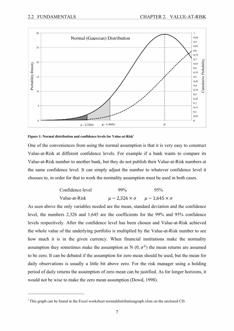
Figure 9: Daily returns and ICSS change points, S&P500 TR index (20.7.1-19.7.11)i

i Computation of this graph and the VBA code for the ICSS algorithm can be found in the Excel worksheet ICSScalculation.xlsm on the enclosed CD.

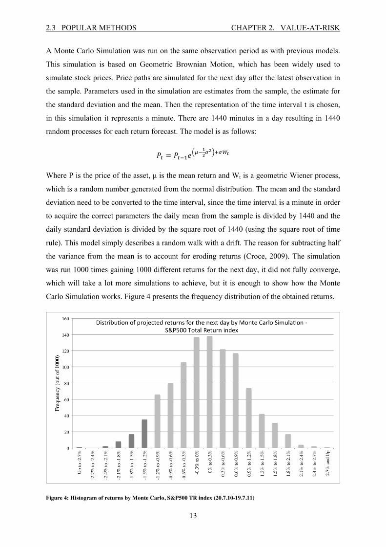
3.2 ARCH CHAPTER 3. TIME-SERIES ANALYSIS

24

By visually examining the change points, it seems that the ICSS algorithm adequately

represents where the variances start to change. It is interesting to see how many change points

are near each other, in and around the start of the financial crisis in late 2008.

3.2 Autoregressive Conditional Heteroskedasticity (ARCH) The ARCH model introduced by Engle in 1982 is designed to tackle the problems of volatility

clustering in time-series therefore making a time-series model that takes account for

heteroskedasticity in the data. It is described as ARCH (q) where q is the number of lagged

values of r2 used in the model, stated as the order of the ARCH process. The ARCH model

can be shown as:

!!!!! = ! + !!!!!!!!!

!

!!!

Where ! and !! are estimated parameters and !!!!! is the conditional (changing) variance.

The error terms, denoted by !!!! are determined by a stochastic value !!!! and a time

dependent conditional standard deviation !!!!.

!!!! = !!!!!!!!

Where !!~! 0,1 and !!!! comes from the original model.

To ensure non-negative volatility, all the alpha values are required to fit this condition (Engle

R. F., 1982):

! > 0  !"#  !!,⋯ ,!! ≥ 0

For !!!!! to ensure wide sense stationarity the parameters are also required to have the

following constraints:

!! + !! +⋯+ !! < 1

When those conditions are satisfied the unconditional (long term) variance becomes existent

and is calculated as (Hamilton, 1994):

!! = ! !!! =!

1− !! − !! −⋯− !!

3.2 ARCH CHAPTER 3. TIME-SERIES ANALYSIS

25

The recursive form of the ARCH (q) model, which in many cases is easier to comprehend is

written as:

!!!!! =  ! + !!!!!!!!! + !!!!!!!!! +⋯+ !!!!!!!!!

The simplest ARCH process would be defined as ARCH (1) and is written as:

!!!!! = ! + !!!!!

For the parameter estimation a regression is needed, based on the maximum likelihood

function. When the likelihood function is maximized based on the sample data and constraints,

the parameters are at the optimal level. The function to be maximized is l, shown below:

! =1! !!

!

!!!

!! = −12 log!!

! −12!!!

!!!

Determined by the order of q lags, the ARCH process accounts for volatility clustering since

it gives weights to the nearest squared returns. However for the ARCH model to converge it

usually needs the order of the ARCH (q) process to be set at a high value. Making the

estimation difficult since when q increases, the number of parameters increases. One of the

solutions to this problem is to make the lagged residuals have linearly decreasing weights,

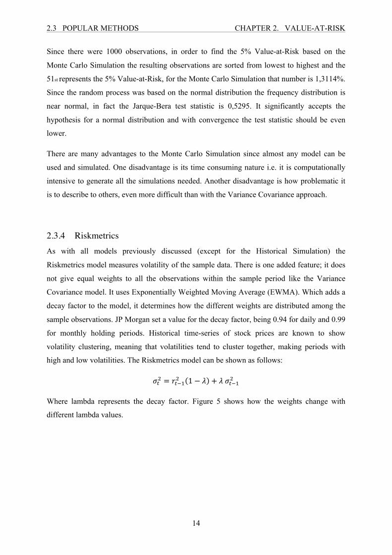
similar to the Riskmetrics model.

!!!!! = ! + ! !!!!!!!!!

!

!!!

Where !! represents the weights given to each residual used in the model. The weights are

calculated using this formula, making the sum of all weights equal to one (Engle R. F., 1982).

!! =2 ! + 1− !! ! + 1

Using this method only two parameters need to be estimated (! and !) making the regression

computationally less intensive. Bollerslev noted that an arbitrary lag structure like this

estimates a totally free lag distribution and therefore does in many cases lead to a violation of

3.3 GARCH CHAPTER 3. TIME-SERIES ANALYSIS

26

the non-negativity constraints. In 1986 Bollerslev presented the GARCH model, described in

the next section (Bollerslev, 1986).

3.3 Generalized Autoregressive Conditional Heteroskedasticity (GARCH) The difficulties with the ARCH process noted by Bollerslev are estimates of a totally free lag

distribution created by the ARCH process, where the number of lags could be high, which

could lead to a violation of the non-negativity constraints. He presented an extension of the

ARCH model denoted as GARCH (p, q) where p represents the order of the GARCH

elements and q represents the order of the ARCH elements. The model looks like this:

!!!!! = ! + !!!!!!!!! + !!!!!!!!!

!

!!!

!

!!!

Where !, !! and !! are parameters to be estimated. Last part of the explanatory variables is

the extension created by a GARCH model. Where lagged conditional variance is a dependent

variable on the conditional variance. To ensure non-negative volatility the following

constraints are added:

p ≥ 0, q > 0,

ω > 0, αi ≥ 0, i = 1,…,q,

βj ≥ 0, j = 1,…,p.

If p is equal to zero, the GARCH model is reduced to an ARCH (q) model (Bollerslev, 1986).

For wide sense stationarity and the variance to be mean reverting, constraint to be added is:

!! + !! < 1

When the variance is mean reverting it converges to the unconditional variance when high

number of forecast steps is used.

The unconditional variance can be calculated as (Engle R. , 2001):

!! =!

1− !! − !! −⋯− !! − !! − !! −⋯− !!

The model takes the recursive form:

3.3 GARCH CHAPTER 3. TIME-SERIES ANALYSIS

27

!!!!! = ! + !!!!!!!!! + !!!!!!!!! +⋯+ !!!!!!!!! + !!!!!!!!! + !!!!!!!!! +⋯+ !!!!!!!!!

A special feature of the GARCH model is that it acts as an infinite order ARCH model

(ARCH (∞)) making it preferable by many since the parameters to be estimated are much

fewer and yield similar results.

The GARCH (1,1), which is most commonly used on financial time-series, is shown as:

!!!!! = ! + !!!! + !!!!

Estimation of parameters for GARCH (p, q) model is same as with ARCH (q) model

(Bollerslev, 1986). Using the same likelihood function shown in section 3.2.

The GARCH model is an important part of this research, where the preferred GARCH (p, q)

model is found by model selection process introduced in section 5.1 and evaluated in section

5.6. This leads to backtesting a set of evaluation methods for Value-at-Risk. Defined and

explained in Chapter 4.

28

4 Backtests

Backtesting is an important part of the Value-at-Risk model evaluation process. It takes the

values that have been calculated by the selected model and tests if the model has been

accurate enough to justify its use on a given portfolio.

The tests are often put in two sets of groups, unconditional coverage and independence.

Unconditional coverage counts the frequencies of violations. A violation is when the actual

return exceeds the Value-at-Risk number for that date. If the Value-at-Risk level were 5%,

from a sample of 100 Value-at-Risk estimates against actual return observations, it would

expect five of them to be violations. The test for independence makes assumption for the

observations to be independent of each other, based on that, when a violation happens for two

or more consecutive days there might be a problem with the model.

Six backtests will be described in the following sections.

4.1 Basel Traffic Light Approach The Basel committee designed a test that banks are regulated to use, it is the Basel Traffic

Light approach, which is an unconditional test. It is set to account for 1% Value-at-Risk with

a holding period of 10 days and an observation period of one year (250 days) for internal

processes of banks. The test can be done with other values as well. The approach is based on

the cumulative binomial distribution and can be shown as:

! ! ≤ ! =!! !! 1− ! !!!

!

!!!

,            !! =

!!!! ! − ! !

Where ! ! ≤ ! represents the probability of violations to be less than or equal to violations

observed, n represents the number of trials (observation period), v represents the observed

violations, t represents cumulative probabilities up to the value of t and p represents the

probability of failure for each trial (p = 0.05 for 5% Value-at-Risk).

The Basel Committee then set out zones that models could fit in, three zones in all: green

zone, yellow zone and red zone. The cumulative probability gives the probability of a correct

model showing fewer or the same amount of violations as have been observed. When the

cumulative probabilities range up to 95% the model is in the green zone, the yellow zone

4.2 KUPIEC TEST CHAPTER 4. BACKTESTS

29

begins when the cumulative probability exceeds 95% and the red zone begins when the

cumulative probability exceeds 99,99%. A model in the green zone is considered to be sound.

If it is in the yellow zone, some investigation is required and probably changes. The red zone

makes the model insufficient and change of operations is needed (Nieppola, 2009). There is

one fault with this model, even though the financial regulators might not care, since it is made

from their perspective. It fails to take into account if violations are too few. It does not matter

what the observation period is or what the level of confidence is set to, the Basel Traffic Light

approach always displays the model in the green zone when there are zero violations up to the

yellow zone threshold level. A model with zero violations is most likely overestimating

Value-at-Risk and that should alarm the risk manager.

4.2 Kupiec Test Kupiec suggested a test in 1995. It is an unconditional coverage test and it measures whether

the number of violations is consistent with the chosen confidence level. The number of

exceptions follows the binomial distribution and it is a hypothesis test, where the null-

hypothesis is:

!!:  ! = ! =!!

Where p represents the violation rate from the chosen Value-at-Risk level, !  represents the

observed violation rate and x represents the number of observed violations. T is the number of

observations. It is conducted as a likelihood-ratio (LR) test and can be formulated as:

!"!" = 2 ln!! 1− ! !!!

!! 1− ! !!! , ! =!!

The test is asymptotically chi-square distributed with one degree of freedom, for a confidence

level of 95% the critical value is 3,84. If the !"!"  statistic exceeds the critical value, the null

hypothesis is rejected and therefore the model seems inaccurate (Néri, 2005).

4.3 CHRISTOFFERSEN TEST CHAPTER 4. BACKTESTS

30

4.3 Christoffersen Test Christoffersen test is an independence test and explained in Christoffersen & Pelletier (2004).

It is a likelihood-ratio test like the Kupiec test. It collects data for violations and if they

happen subsequently. The results from this data collection are used to create the test results.

The observations can have two values as shown below.

!! =1, !"  !"#$%&"#'  !""#$%0, !"  !"  !"#$%&"#'  !""#$%

A violation occurs when the actual returns exceed the projected Value-at-Risk number

!! < −!"#! . Those results are categorized in the following manner: if there was a violation

followed by non violation, a non violation followed by a violation, a non violation followed

by a non violation and a violation followed by a violation, as shown below:

It-1 = 0 It-1 = 1

It = 0 n00 n10 n00 + n10

It = 1 n01 n11 n01 + n11

n00 + n01 n10 + n11 N

From the table above, values for !! and !! are calculated where they represent the sample

probabilities of a violation occurring conditional on if there was or was not a violation in the

previous day. ! is then also calculated and represents the violation rate, as shown below:

!! =!!"

!!! + !!",            !! =

!!!!!" + !!!

           !"#            ! =!!" + !!!

!!! + !!" + !!" + !!!  

The likelihood-ratio test is calculated under the null-hypothesis that all violations should be

independent of each other. The null-hypothesis takes the form:

Η!:  !! = !!

The likelihood statistics is calculated as:

!"!"# = −2 ln1− ! !!!!!!"!!!"!!!!

1− !! !!!!!!!" 1− !! !!"!!

!!!

Which is asymptotically chi-square distributed with one degree of freedom, making the

critical value at 95% confidence interval 3,84. If the test statistics is above that value the null-

hypothesis is rejected and the model is thought to have independence problems. A test

statistic under the critical rate assumes the model to be sound (Nieppola, 2009).

4.4 TEST FOR CONDITIONAL COVERAGE CHAPTER 4. BACKTESTS

31

4.4 Test for Conditional Coverage Christoffersen created a joint test consisting of the previously described tests for

unconditional coverage and for independence. The test statistic is as follows:

!"!! = !"!" + !"!"#

Kupiec test for unconditional coverage and Christoffersen test for independence are summed

to get the test results for conditional coverage. The test for conditional coverage is also

asymptotically chi-square distributed and has two degrees of freedom. The critical value at

95% confidence level is 5,99. Making the model pass the test if its test statistic is under the

critical value (Christoffersen & Pelletier, 2004).

4.5 Pearson’s Q Test Although the previously discussed backtests can all be considered to be adequate, there is one

thing they are lacking. They don’t test simultaneously the predicted Value-at-Risk for

multiple confidence levels, that can be done with the Pearson’s Q test for goodness of fit. To

run the test, first the chosen confidence levels that are tested simultaneously should be

specified, and separated into bins. If it is for instance decided to test Value-at-Risk at 95%

and 99% confidence levels, the bins should be [0.00, 0.01], [0.01, 0.05] and [0.05, 1.00].

Where all the violations over the 99% confidence level are in the [0.00, 0.01] bin, violations

in between the 99% and 95% confidence levels are in the [0.01, 0.05] bin and the rest (returns

that are lower than the predicted 5% Value-at-Risk loss) are in the [0.05, 1.00] bin. The Q test

is then computed according to the following formula:

! =! !!,!! − ! !! − !!

!

! !! − !!

!

!!!

Where ! !!,!! represents the number of observations in the ith bin and N represents the total

number of observations in the whole test. !! and !! represent the upper and lower bounds of

each bin. The test is asymptotically chi-square distributed with k-1 degrees of freedom. If the

test would be conducted on the 1% and 5% Value-at-Risk levels the critical value will be 5,99

(given 95% confidence) and if the test results are above that value, the model is rejected

(Campbell, 2005).

4.6 LOPEZ’S LOSS FUNCTION CHAPTER 4. BACKTESTS

32

4.6 Lopez’s Loss Function Lopez proposed a magnitude loss function in 1999. It is neither an independence test nor a

test for unconditional coverage. Looking at the losses made when there is a violation and by

how much the losses exceed the projected Value-at-Risk number. Every observation gets a

value, similar to the independence test where every violation got a value of one otherwise

zero. For observations with no violation the value is set at zero, alternatively when there is a

violation the value is one plus the magnitude of the exceedance squared. As shown below:

! !"#! ! , !! = 1+   !! + !"#! !!, !"  !"#!"#$%&  !""#$%0, !"  !"  !"#$%&"#'  !""#$%

Where !"#! ! represents the projected Value-at-Risk number for time t, ! represents the

chosen confidence level and !! is the observed return at time t.

To get a single value, the results are calculated using the following formula:

! =1! ! !"#! ! , !!

!

!!!

There are some shortfalls with the Lopez Loss function, since the actual distribution of the

returns is unknown. It is hard to know how much exceedance is actually appropriate and how

much leads to a rejection of the model. The Loss function is good though for comparing

different models and to see if there are some extraordinary exceedances prevailing (Lopez,

1999).

33

5 Empirical Research

This research will use the S&P500 Total Return index, ranging from 20.07.01-19.07.11

making a total of 10 years and 2512 observations. Returns in the data that showed zero were

taken out (holidays). Additionally, one week has been removed because of closed markets. It

is the week right after the September 11th attacks on the World Trade Center in the United

States.

The returns are calculated continuously, following the given description:

!! = ln!!!!!!

Where !! represents the returns at time t and S represents the index rate at the given time.

The preferred GARCH (p, q) model will be found based on the model selection process. The

most widely used model GARCH (1, 1) will be evaluated in this research regardless of what

model will be selected. The models will be compared to the Riskmetrics model with a lambda

value of 0,94.

Calculations will be in Excel and VBA. Additionally MATLAB mathematical and statistical

software will be utilized. The VBA codes are available in appendix A.

The next section will go into the model selection process, which determines how different

GARCH models perform against each other.

5.1 Model Selection Process There will be two types of tests performed on the returns series to see which GARCH model

is considered most fitting on the time-series. The tests are Akaike Information Criterion (AIC)

and Schwartz Bayesian Criterion (SBC). The preferred model will show the lowest values of

these criterions. The main difference between the criterions is that SBC penalizes models

more when number of parameters increases. The AIC is calculated as:

!"# =  −2! !!! + 2!

5.1 MODEL SELECTION PROCESS CHAPTER 5. EMPIRICAL RESEARCH

34

Where K is the number of free parameters to be estimated in the model and ! !!! is the

likelihood function. For a GARCH (1, 1) model the K would equal 3 since omega, beta and

alpha are estimated. The SBC criterion is similar and can be shown as:

!"# =  −2! !!! + ! ln !

Where n represents the number of residuals in the model, the data has 2512. The AIC and

SBC were calculated for GARCH model with the least possible parameters and up to

GARCH (3, 3) the results are shown in the table below:

AIC and SBC statistics for GARCH models

Model AIC SBC

GARCH (0,1) -14776,786 -14759,299

GARCH (1,1) -15834,083 -15810,768

GARCH (2,1) -15832,083 -15802,939

GARCH (1,2) -15862,874 -15833,730

GARCH (2,2) -15860,873 -15825,900

GARCH (3,1) -15830,085 -15795,112

GARCH (3,2) -15858,874 -15818,072

GARCH (1,3) -15861,634 -15826,661

GARCH (2,3) -15859,721 -15818,919

GARCH (3,3) -15857,721 -15811,090 Table 2: AIC and SBC statistics for various GARCH modelsi

The strongest model based on both the AIC and SBC is the GARCH (1, 2) model, which can

be expressed as:

!!!!! = ! + !!!!! + !!!!!!! + !!!!

To further examine the GARCH (1, 2), parameter estimations need to be calculated with

regression statistics, the results are shown in table 3:

i The mathematical and statistical software MATLAB was used to attain the AIC and SBC statistics.

5.1 MODEL SELECTION PROCESS CHAPTER 5. EMPIRICAL RESEARCH

35

Estimated parameters for the GARCH (1, 2) model

Parameter Value Standard Error T-Statistic P-value

! 1,8984e-006 3,2028e-007 5,9272 0,0000***

!! 0 0,015413 0,0000 1,0000

!! 0,1035 0,018373 5,6331 0,0000***

! 0,885 0,012099 72,9396 0,0000***

Likelihood 7936,4370398 Table 3: Estimated parameters for the GARCH (1, 2) modeli

Note: * p < .05; ** p < .01; *** p < .001

It is interesting to see that the value for !! is zero and the T-statistic is zero making the p-

value go up to 1, accepting the null-hypothesis for the estimate to be zero and therefore not

contributing to the model, which is quite surprising, one would think that the first lagged

residual will have some explanatory power. When the estimated parameters are inputted the

model looks as follows:

!!!!! = 0,0000018984+ 0  ×  !!! + 0,1035  ×  !!!!! + 0,885  ×  !!!

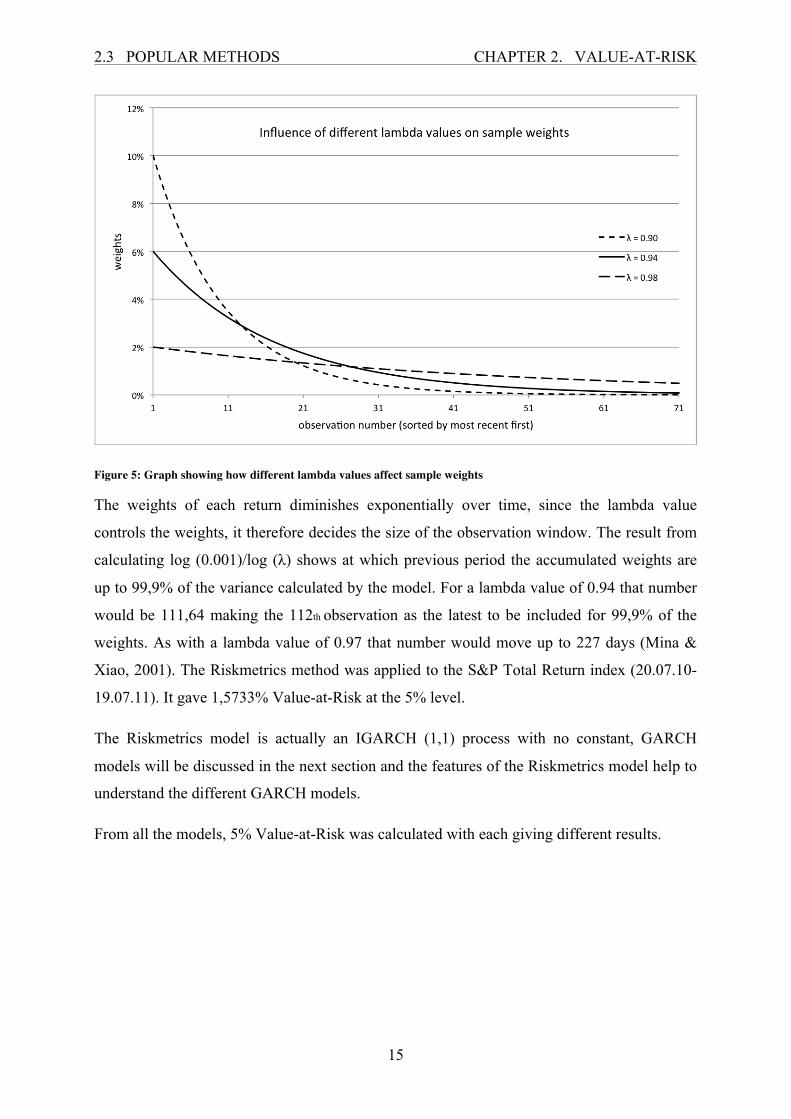
Here the parameter values are shown in the model, to explain their functions. ! is the

conditional variance constant, the conditional variance being what the GARCH model is

measuring. !! is the coefficient related to the lagged residuals squared, !! would then

represent the weight that is put on the latest observation squared. !! represents the weight that

is put on the second latest observation squared and so forth. ! represents the coefficient

related to the lagged conditional variance. Its value represents the weight that is put on the

latest lagged conditional variance. Since there is only one beta to be estimated in the GARCH

(1, 2) model it is given the parameter !. If there would be more than one beta to be estimated,

as is in GARCH (p > 1, q) models. The coefficient or weight for the first lagged conditional

variance would get the parameter !!, the second !! and so forth.

Since this model can be explained as GARCH (1, 1) model with an extra ARCH parameter

the GARCH (1, 1) model is nested within it. The GARCH (1, 1) model is usually the

preferred model for financial time-series making it interesting to compare those two by the

i The mathematical and statistical software MATLAB was used to estimate the parameters for the GARCH (1, 2), restricted GARCH (1, 2) and the GARCH (1, 1) models.

5.1 MODEL SELECTION PROCESS CHAPTER 5. EMPIRICAL RESEARCH

36

Likelihood Ratio Test. In order to do that, first the parameter estimation for the GARCH (1,

1) is calculated, primarily to get the likelihood. Shown in table 4.

Estimated parameters for the GARCH (1, 1) model

Parameter Value Standard Error T-Statistic P-value

! 1,2207e-006 2,1058e-007 2,8115 0,0050**

! 0,075626 0,0079575 9,5037 0,0000***

! 0,9155 0,008567 106,8640 0,0000***

Likelihood 7921,0415508 Table 4: Estimated parameters for the GARCH (1, 1) model

Note: * p < .05; ** p < .01; *** p < .001

Based on the estimation results, all the p-values are very low, rejecting the null-hypothesis for

the estimations to be zero, making the model a good fit. The model can be shown as:

!!!!! = 0,0000012207+ 0,075626  ×  !!! + 0,9155×  !!!

This model has already been compared to the GARCH (1, 2) model with the AIC and SBC

where the GARCH (1, 2) resulted in lower values, making it seem to be a better fit. To further

test the models against each other the Likelihood Ratio Test is conducted, it can be shown as:

2 !! − !! ≈ !! !

Where !! is the value of the likelihood function for the unrestricted model, !! is the value of

the likelihood function for the restricted model and ! is the number of restrictions put on the

unrestricted model. The null-hypothesis is that the restricted model is the “true” model. The

test is asymptotically chis-square distributed with ! degrees of freedom (Hamilton, 1994).

Plotting the likelihood results, shown in tables 3 and 4, from the unrestricted (GARCH (1, 1))

and the restricted (GARCH (1, 2)) model. We get a test result of 30,8 significantly rejecting

null-hypothesis of GARCH (1, 1) model being the “true” model and therefore strengthening

results from the AIC and SBC. The critical rate at 95% confidence interval was 3,814 given

one degree of freedom, since the restricted model reduced the unrestricted model by one

parameter.

From the estimation of the GARCH (1, 2) model in table 3 it was interesting to see that the

estimated parameter for the weights on the first lagged residual was zero and very

significantly so, according to its p-value. Because of that, a new estimation was run where

5.1 MODEL SELECTION PROCESS CHAPTER 5. EMPIRICAL RESEARCH

37

this parameter was dropped that could lead to a stronger model. The new model will be called

restricted GARCH (1, 2). The regressions statistics, AIC and SBC for the new model are

shown below:

Estimated parameters for the restricted GARCH (1, 2) model

Parameter Value Standard Error T-Statistic P-value

! 1,9054e-006 3,197e-007 5,9600 0,0000***

!! 0,10339 0,011168 9,2581 0,0000***

! 0,88238 0,012059 73,1692 0,0000***

Likelihood 7936,4377438

AIC -15864,875

SBC -15841,560 Table 5: Estimated parameters for the restricted GARCH (1, 2) model

Note: * p < .05; ** p < .01; *** p < .001

All the estimated parameters are significant with more than 99,9% confidence.

Both the AIC and SBC penalize models more when the number of free parameters increases,

that contributes to why they show better results for the restricted GARCH (1, 2) model than

with unrestricted. According to the AIC and SBC values the restricted GARCH (1, 2) model

is more fitting to the sample than the GARCH (1, 2) model, when all the parameter estimates

are inputted, the model looks as follows:

!!!!! = 0,0000019054+ 0,10339  ×  !!!!! + 0,88238  ×  !!!

The most interesting thing about this model specification is that the only squared residual that

is weighted to attain the conditional variance, is the second lagged residual squared. The most

recent one is left out of the equation.

To further test this model against the GARCH (1, 2) the Likelihood Ratio Test was conducted

where this is the restricted model and GARCH (1, 2) is the unrestricted model. It is interesting

to compare the likelihoods, for the restricted GARCH (1, 2) the likelihood is higher than for

the GARCH (1, 2) model. Usually the likelihood of the model that is nested within the other

has a lower likelihood but here it is not the case. The Likelihood ratio test was conducted on

these two models giving a test result of -0,0014; with a 95% critical value of 3,814 the null-

hypothesis is very significantly accepted for the restricted model to be the “true” model.

5.2 LJUNG-BOX Q TEST CHAPTER 5. EMPIRICAL RESEARCH

38

The restricted GARCH (1, 2) model will therefore be selected. As previously mentioned, even

though the GARCH (1, 1) model was not chosen in the model selection process it will be used

and evaluated against the restricted GARCH (1, 2), and the Riskmetrics model.

In the next two sections the Ljung-Box Q test and the test for ARCH effects introduced by

Engle will be conducted on the residuals of the GARCH (1, 1) and the restricted GARCH (1,

2) models.

5.2 Ljung-Box Q Test The Ljung-Box Q test has already been performed on the original sample, it is interesting to

see how the autocorrelations with the residuals of a given model perform under the same test.

This hypothesis test, which tests if there is any autocorrelation up to a predefined lag was

performed on the GARCH (1, 1) and the restricted GARCH (1, 2) models. The null-

hypothesis states that there is no autocorrelation in the residuals and if the null-hypothesis is

rejected, if at least one autocorrelation is not zero (Ljung & Box, 1978). The formula used is

the same as before:

!! = ! ! + 2 !!! ∕ ! − !!

!!!

Where !!! represents autocorrelations for the residuals at lag j. The test is asymptotically chi-

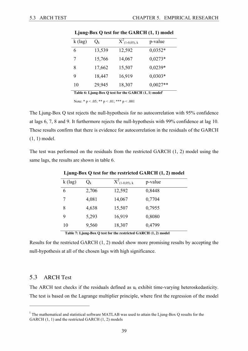
square distributed with k degrees of freedom. Table 6 shows the results for the residuals from

the GARCH (1, 1) model for the same lags as was used on the returns in section 6 (lags 6, 7, 8,

9 and 10).

5.3 ARCH TEST CHAPTER 5. EMPIRICAL RESEARCH

39

Ljung-Box Q test for the GARCH (1, 1) model

k (lag) Qk X2(1-0,05), k p-value

6 13,539 12,592 0,0352*

7 15,766 14,067 0,0273*

8 17,662 15,507 0,0239*

9 18,447 16,919 0,0303*

10 29,945 18,307 0,0027** Table 6: Ljung-Box Q test for the GARCH (1, 1) modeli

Note: * p < .05; ** p < .01; *** p < .001

The Ljung-Box Q test rejects the null-hypothesis for no autocorrelation with 95% confidence

at lags 6, 7, 8 and 9. It furthermore rejects the null-hypothesis with 99% confidence at lag 10.

These results confirm that there is evidence for autocorrelation in the residuals of the GARCH

(1, 1) model.

The test was performed on the residuals from the restricted GARCH (1, 2) model using the

same lags, the results are shown in table 6.

Ljung-Box Q test for the restricted GARCH (1, 2) model

k (lag) Qk X2(1-0,05), k p-value

6 2,706 12,592 0,8448

7 4,081 14,067 0,7704

8 4,638 15,507 0,7955

9 5,293 16,919 0,8080

10 9,560 18,307 0,4799 Table 7: Ljung-Box Q test for the restricted GARCH (1, 2) model

Results for the restricted GARCH (1, 2) model show more promising results by accepting the

null-hypothesis at all of the chosen lags with high significance.

5.3 ARCH Test The ARCH test checks if the residuals defined as ut exhibit time-varying heteroskedasticity.

The test is based on the Lagrange multiplier principle, where first the regression of the model

i The mathematical and statistical software MATLAB was used to attain the Ljung-Box Q results for the GARCH (1, 1) and the restricted GARCH (1, 2) models

5.3 ARCH TEST CHAPTER 5. EMPIRICAL RESEARCH

40

is calculated, in order to get the residuals. When the model specification is complete and the

residuals attained, !!! is regressed on a constant and m of its own lagged values:

!!! =  ! + !!!!!!! + !!!!!!! +⋯+ !!! !!!!! + !!

For t = 1, 2, …, T. The statistics can be reviewed under the chi-square distribution with m

degrees of freedom with the null-hypothesis being that there is no heteroskedasticity present

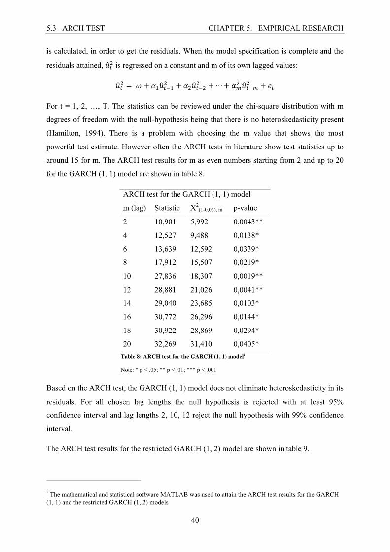
(Hamilton, 1994). There is a problem with choosing the m value that shows the most

powerful test estimate. However often the ARCH tests in literature show test statistics up to

around 15 for m. The ARCH test results for m as even numbers starting from 2 and up to 20

for the GARCH (1, 1) model are shown in table 8.

ARCH test for the GARCH (1, 1) model

m (lag) Statistic X2(1-0,05), m p-value

2 10,901 5,992 0,0043**

4 12,527 9,488 0,0138*

6 13,639 12,592 0,0339*

8 17,912 15,507 0,0219*

10 27,836 18,307 0,0019**

12 28,881 21,026 0,0041**

14 29,040 23,685 0,0103*

16 30,772 26,296 0,0144*

18 30,922 28,869 0,0294*

20 32,269 31,410 0,0405* Table 8: ARCH test for the GARCH (1, 1) modeli

Note: * p < .05; ** p < .01; *** p < .001

Based on the ARCH test, the GARCH (1, 1) model does not eliminate heteroskedasticity in its

residuals. For all chosen lag lengths the null hypothesis is rejected with at least 95%

confidence interval and lag lengths 2, 10, 12 reject the null hypothesis with 99% confidence

interval.

The ARCH test results for the restricted GARCH (1, 2) model are shown in table 9.

i The mathematical and statistical software MATLAB was used to attain the ARCH test results for the GARCH (1, 1) and the restricted GARCH (1, 2) models

5.4 PARAMETER ESTIMATION CHAPTER 5. EMPIRICAL RESEARCH

41

ARCH test for the restricted GARCH (1, 2) model

m (lag) Statistic X2(1-0,05), m p-value

2 1,653 5,992 0,4377

4 1,720 9,488 0,7871

6 2,705 12,592 0,8448

8 4,603 15,507 0,7991

10 9,906 18,307 0,4488

12 11,092 21,026 0,5210

14 11,371 23,685 0,6567

16 12,530 26,296 0,7068

18 12,545 28,869 0,8179

20 14,309 31,410 0,8145 Table 9: ARCH test for the restricted GARCH (1, 2) model

The null-hypothesis is accepted at all lag levels, so the restricted GARCH (1, 2) model does

not show any signs of heterskedasticity in its residuals.

These results, from both the Ljung-Box Q test and the ARCH test indicate that the restricted

GARCH (1, 2) model is a better fit for the time-series, than the GARCH (1, 1) model. Its

residuals show no evident sign of autocorrelation or heterskedasticity whereas the GARCH (1,

1) model does so in both cases.

5.4 Parameter Estimationi The estimation of the parameters for the GARCH (1, 1) model and the GARCH (1, 2) models

used a rolling parameter estimation window. Throughout the returns series, for each day there

will be a new value estimated for the parameters based on window size, which “rolls” up the

time-series. There is a VBA algorithm that calculates these estimates automatically. It is

called the Nelder-Mead algorithm, which minimizes a function containing more than one

parameter to be estimated. Since the likelihood function for the GARCH models needs to be

maximized, the objective function in the algorithm was defined as the negative of that

i Parameter estimation for the Riskmetrics model and all rolling window sizes for the GARCH models can be found in Excel worksheets in the sub-folder “variances” on the enclosed CD. It is recommended to either set calculation preferences in Excel to “manual” before opening the files or to disable macros when opening the files. Otherwise Excel might start recalculating the whole worksheet, which might take a few hours.

5.5 BACKTEST SAMPLES CHAPTER 5. EMPIRICAL RESEARCH

42

function. The equality constraints for the GARCH models were added. The VBA code for this

algorithm is from the book Option Pricing Models & Volatility (Rouah & Vainberg, 2007).

The main problem with using rolling parameter estimation is to find the optimal window size.

It might vary depending on the state of the time-series since financial time-series exhibit

volatility clustering. If a drastic change in volatility happens and before that volatility had

been near constant, then the model estimation could rely too heavily on how the volatilities

had been in the previous period.

There is an idea to use the ICSS algorithm to find the volatility change points and then adjust

the model accordingly for every new point. The ICSS algorithm is applied on a small sub-

sample at the beginning of the S&P500 Total Return index sample and run several times. For

each run the range is incremented by one day, until a new change point is discovered. For

each change point, the date for which the range has gone up to is marked and checked how far

away that date was from the change point. That date will then represent the time when a new

change point is found in practice by applying the ICSS algorithm. If it is close enough to the

change point, the model can be adapted accordingly. Otherwise too much time has passed for

an adjustment of the model to adequately cover the change of variance. This test found that

the time between the change points and the dates they were realized on could range from ≈ 30

days up to ≈ 300 days. Therefore, it cannot be assumed that a change point will be realized

around the time it takes place, by the use of the ICSS algorithm. That’s why no adjustments

will be made to the models.

Because of how difficult it is to find the optimal window size for a rolling GARCH model,

the models were estimated with multiple window sizes: 250, 500, 750, 1000, 1250 and 1500.

Resulting in six different estimates for each of the GARCH models. The Riskmetrics model

was set with a lambda value of 0,94 making consideration for window sizes unnecessary.

5.5 Backtest Samples For backtesting purposes the data is split into two sub-samples, each of them is backtested

along with the full sample. The full sample of the S&P500 Total Return index, ranging from

20.07.10 to 19.07.11 giving 2512 observations in total. The financial crisis of late 2008 is in

the sample, this was a good opportunity to test how the different models performed in the

midst of the crisis, to see how the models perform in turbulent times. Since the ICSS

5.5 BACKTEST SAMPLES CHAPTER 5. EMPIRICAL RESEARCH

43

algorithm had already been applied on the Full sample, there is information present on the

variance change points in the Full sample. Let the change points be defined as with the ICSS

algorithm, a total of seven change points in the Full sample, so the first change point would be

defined !"! second !"! and so forth up to the last !"!. Furthermore, !"! is the start of the

sample and !"! is the end of the sample.

By examining the change points it is evident that five of them are relatively close to each

other around the time of the financial crisis, these points range from !"! to !"!. The first !"!

and the last !"! mark the boundaries of the sample used for backtesting the financial crisis.

That sample will start from !"! and go up to !"! minus one day. Giving a sample range from

09.07.07 to 03.09.10, a total of 797 observations.

The last sample used for backtesting purposes will be the part that did not show as turbulent

times and could be considered normal. This sample starts from !"! and ends at the start of the

crisis sample at !"! minus one day. This sample ranges from 20.07.01 to 06.07.07 giving a

total of 1496 observations.

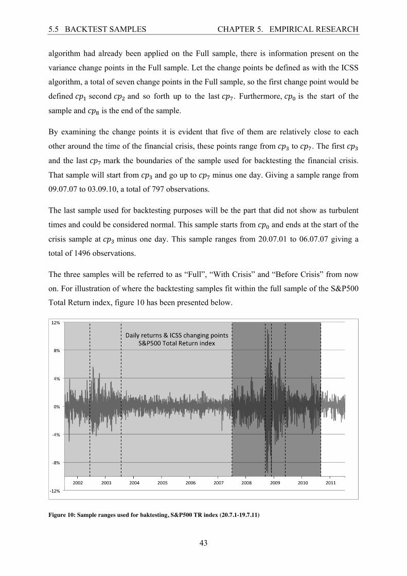
The three samples will be referred to as “Full”, “With Crisis” and “Before Crisis” from now

on. For illustration of where the backtesting samples fit within the full sample of the S&P500

Total Return index, figure 10 has been presented below.

Figure 10: Sample ranges used for baktesting, S&P500 TR index (20.7.1-19.7.11)

5.6 BACKTEST RESULTS CHAPTER 5. EMPIRICAL RESEARCH

44

It is the graph shown in section 3.1, with the areas for each sample dimmed differently. The

darkest part represents the With Crisis sample, the slightly dimmed part represents the Before

Crisis sample and all areas (dark grey, light grey and white) put together represents the Full

sample.

5.6 Backtest Resultsi The backtests were performed on the various models used in this research (on 5% and 1%

Value-at-Risk levels). First the different window sizes of the GARCH (1, 1) and the GARCH

(1, 2) model, were compared to each other and then the window size for each model that

performed best according to the backtests was chosen. This was done for each of the models

to have only one set of estimations for comparison. Among the GARCH (1, 1) the window

size that performed best was of 1500 and for the restricted GARCH (1, 2) estimations it was

500. In this section the results will therefore be shown for the rolling GARCH (1, 1) with a

window size of 1500, the rolling restricted GARCH (1, 2) with a window size of 500 and the

Riskmetrics model.

Statistics from all tests except for the Basel Traffic Light approach are shown. That is because

of similarities between the Basel Traffic Light approach and the test for unconditional

coverage and the fact that the test for unconditional coverage does penalize models with too

few violations where the Basel Traffic Light does not. The results from the tests are shown

based on what part of the sample is tested for, starting with the Full sample. Furthermore, the

results from the Lopez’s loss function are presented in section 5.6.4 where the results are

accompanied with graphs.

i All backtests can be found in Excel worksheets in the sub-folder “backtests” on the enclosed CD.

5.6 BACKTEST RESULTS CHAPTER 5. EMPIRICAL RESEARCH

45

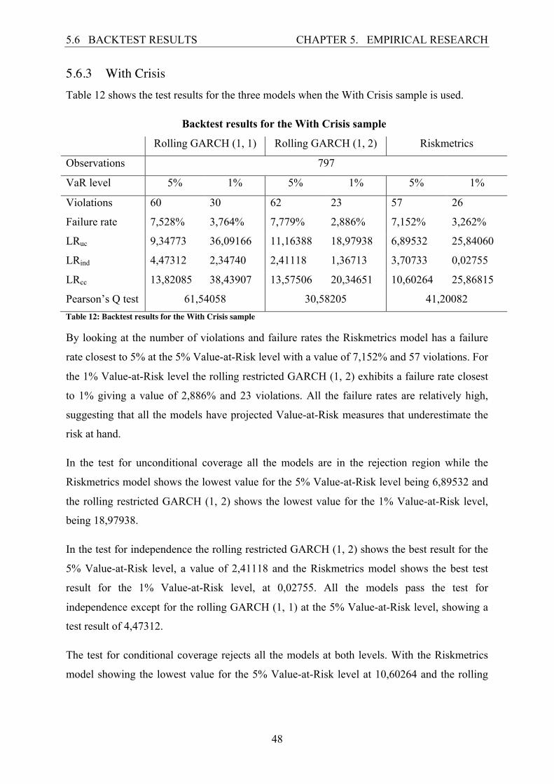
5.6.1 Full Table 10 shows the test results for the three models when the Full sample is used.

Backtest results for the Full sample

Rolling GARCH (1, 1) Rolling GARCH (1, 2)i Riskmetrics

Observations 2512

VaR level 5% 1% 5% 1% 5% 1%

Violations 133 44 137 47 146 48

Failure rate 5,295% 1,752% 5,454% 1,871% 5,812% 1,911%

LRuc 0,45064 11,70992 1,05930 15,32250 3,32216 16,61467

LRind 0,18002 1,56896 0,03396 1,10093 0,03188 0,00755

LRcc 0,63065 13,27889 1,09326 16,42342 3,35404 16,62223

Pearson’s Q test 15,52462 20,20541 21,07534 Table 10: Backtest results for the Full sample

By looking at the number of violations and failure rates for each graph for the 1% and 5%

Value-at-Risk predictions. The rolling GARCH (1, 1) has the failure rate closest to 5% and

1% with 133 and 44 violations, a failure rate of 5,295% and 1,752% respectively.

The test for unconditional coverage is lowest for the rolling GARCH (1, 1) with a value of

0,45064 at the 5% Value-at-Risk level and 11,70992 at the 1% level. The 95% confidence

critical rate is 3,842 so the model cannot be rejected at the 5% Value-at-Risk level, the test

results are also under the critical rate for the 5% Value-at-Risk level. However all the models

fail to fall under the critical level at the 1% Value-at-Risk level.

In the test for independence, the Riskmetrics model shows the lowest value at the 5% and the

1% Value-at-Risk levels, showing values of 0,03188 and 0,00755 respectively. The critical

level is the same as with the test for unconditional coverage and it scores well under that rate

at both 1% and 5% Value-at-Risk levels. Both the other models do also show low values for

the test for independence and fall under the critical rate.

In the test for conditional coverage, the rolling GARCH (1, 1) gives the best results for both

Value-at-Risk levels, 0,63065 for the 5% Value-at-Risk level and 13,27889 1% making it fall

under the critical value of 5,992 at the 5% Value-at-Risk level but goes over it at the 1%

i In this table and the following tables the rolling restricted GARCH (1, 2) model will be named Rolling GARCH (1, 2).

5.6 BACKTEST RESULTS CHAPTER 5. EMPIRICAL RESEARCH

46

Value-at-Risk level and is therefore rejected. The other two models are rejected at the 1%

Value-at-Risk level and pass the test at the 5% Value-at-Risk level.

The model showing the best results for the Pearson’s Q test, although not sufficient with

5,992 as the critical rate, is the rolling GARCH (1, 1) model with a value of 15,5246.

Based on these results, the model that performed best for the Full sample was the rolling

GARCH (1, 1) model, performing well at the 5% Value-at-Risk level. However it did not

perform as well at the 1% Value-at-Risk level, seeing rejection in the test for unconditional

and conditional coverage, and it was rejected in the Pearson’s Q test. Despite that it showed

the best results at the 1% Value-at-Risk level. The other two models did pass all the tests at

the 5% Value-at-Risk level.

5.6.2 Before Crisis Table 11 shows the test results for the three models when the Before Crisis sample is used.

Backtest results for the Before Crisis sample

Rolling GARCH (1, 1) Rolling GARCH (1, 2) Riskmetrics

Observations 1496

VaR level 5% 1% 5% 1% 5% 1%

Violations 62 11 64 21 75 19

Failure rate 4,144% 0,740% 4,280% 1,404% 5,01% 1,270%

LRuc 2,44218 1,16592 1,72221 2,18865 0,00056 1,01527

LRind 2,00209 0,16296 1,67103 4,53910 2,52788 0,48884

LRcc 4,44427 1,32888 3,39324 6,72775 2,52844 1,50411

Pearson’s Q test 2,46943 7,25975 1.33746 Table 11: Backtest results for the Before Crisis sample

The numbers of violations and failure rates seem to be closest to the 5% and 1% levels for the

Riskmetrics model. Giving a failure rate of 5,01% with 75 violations and 1,270% with 19

violations for the 5% and 1% Value-at-Risk levels respectively. The rolling GARCH (1, 1)

model shows a failure rate of 0,740% at the 1% Value-at-Risk level, which has a similar

closeness to the 1% as the Riskmetrics.

5.6 BACKTEST RESULTS CHAPTER 5. EMPIRICAL RESEARCH

47

The test for unconditional coverage gives the best scores for the Riskmetrics at both Value-at-

Risk levels, 0,00056 for the 5% level and 1,01527 for the 1% level. All the models pass the

test for unconditional coverage at both Value-at-Risk levels.

In the test for independence the rolling GARCH (1, 1) shows the best results, giving a value

of 2,00209 for the 5% Value-at-Risk level and 0,16296 for the 1% Value-at-Risk level. The

other models pass the test for independence except for the rolling restricted GARCH (1, 2) at

the 1% Value-at-Risk level, it measures 4,53910 exceeding the critical rate of 3,842.

The test for conditional coverage shows the best results for the Riskmetrics model at both

levels, giving a value of 2,52844 and 1,50411 for the 5% and 1% Value-at-Risk levels

respectively. The other models pass the test for conditional coverage at all levels except for

the rolling restricted GARCH (1, 2) model at the 1% Value-at-Risk level, showing a value of

6,72775, which exceeds the critical level set at 5,992. This is largely because of the poor test

statistics from the test for independence.

The Pearson’s Q test shows the lowest value for the Riskmetrics model, being 1,33746.

Passing the test where the critical rate is set at 5,992. The Rolling GARCH (1, 1) did pass the

test, however the rolling restricted GARCH (1, 2) did not pass the Pearson’s Q test with a

value of 7,25975.

Based on the results, the model that performed best for the Before Crisis sample was the

Riskmetrics model. The models passed all tests, except for the rolling restricted GARCH (1,

2) which did not pass test for independence and conditional coverage for Value-at-Risk level

of 1%. Additionally it faced rejection in Pearson’s Q test.

5.6 BACKTEST RESULTS CHAPTER 5. EMPIRICAL RESEARCH

48

5.6.3 With Crisis Table 12 shows the test results for the three models when the With Crisis sample is used.

Backtest results for the With Crisis sample

Rolling GARCH (1, 1) Rolling GARCH (1, 2) Riskmetrics

Observations 797

VaR level 5% 1% 5% 1% 5% 1%

Violations 60 30 62 23 57 26

Failure rate 7,528% 3,764% 7,779% 2,886% 7,152% 3,262%

LRuc 9,34773 36,09166 11,16388 18,97938 6,89532 25,84060

LRind 4,47312 2,34740 2,41118 1,36713 3,70733 0,02755

LRcc 13,82085 38,43907 13,57506 20,34651 10,60264 25,86815

Pearson’s Q test 61,54058 30,58205 41,20082 Table 12: Backtest results for the With Crisis sample

By looking at the number of violations and failure rates the Riskmetrics model has a failure

rate closest to 5% at the 5% Value-at-Risk level with a value of 7,152% and 57 violations. For

the 1% Value-at-Risk level the rolling restricted GARCH (1, 2) exhibits a failure rate closest

to 1% giving a value of 2,886% and 23 violations. All the failure rates are relatively high,

suggesting that all the models have projected Value-at-Risk measures that underestimate the

risk at hand.

In the test for unconditional coverage all the models are in the rejection region while the

Riskmetrics model shows the lowest value for the 5% Value-at-Risk level being 6,89532 and

the rolling restricted GARCH (1, 2) shows the lowest value for the 1% Value-at-Risk level,

being 18,97938.

In the test for independence the rolling restricted GARCH (1, 2) shows the best result for the

5% Value-at-Risk level, a value of 2,41118 and the Riskmetrics model shows the best test

result for the 1% Value-at-Risk level, at 0,02755. All the models pass the test for

independence except for the rolling GARCH (1, 1) at the 5% Value-at-Risk level, showing a

test result of 4,47312.

The test for conditional coverage rejects all the models at both levels. With the Riskmetrics

model showing the lowest value for the 5% Value-at-Risk level at 10,60264 and the rolling

5.6 BACKTEST RESULTS CHAPTER 5. EMPIRICAL RESEARCH

49

restricted GARCH (1, 2) shows the lowest value for the 1% Value-at-Risk level, which is

13,57506.

The Pearson’s Q test rejects all the models where the rolling restricted GARCH (1, 2) shows

the lowest value of 30,58205.

From these results, none of the models managed to mitigate risk for the period with the

financial crisis. This is a main pitfall of Value-at-Risk models, it is hard to find a model that

efficiently forecasts risk during turbulent times. This comparison shows that the rolling

restricted GARCH (1, 2) model performed best for the With Crisis sample.

5.6 BACKTEST RESULTS CHAPTER 5. EMPIRICAL RESEARCH

50

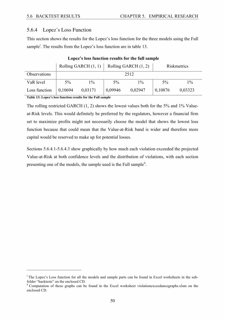
5.6.4 Lopez’s Loss Function This section shows the results for the Lopez’s loss function for the three models using the Full

samplei. The results from the Lopez’s loss function are in table 13.

Lopez’s loss function results for the full sample

Rolling GARCH (1, 1) Rolling GARCH (1, 2) Riskmetrics

Observations 2512

VaR level 5% 1% 5% 1% 5% 1%

Loss function 0,10694 0,03171 0,09946 0,02947 0,10876 0,03323 Table 13: Lopez’s loss function results for the Full sample

The rolling restricted GARCH (1, 2) shows the lowest values both for the 5% and 1% Value-

at-Risk levels. This would definitely be preferred by the regulators, however a financial firm

set to maximize profits might not necessarily choose the model that shows the lowest loss

function because that could mean that the Value-at-Risk band is wider and therefore more

capital would be reserved to make up for potential losses.

Sections 5.6.4.1-5.6.4.3 show graphically by how much each violation exceeded the projected

Value-at-Risk at both confidence levels and the distribution of violations, with each section

presenting one of the models, the sample used is the Full sampleii.

i The Lopez’s Loss function for all the models and sample parts can be found in Excel worksheets in the sub-folder “backtests” on the enclosed CD. ii Computation of these graphs can be found in the Excel worksheet violationexceedancegraphs.xlsm on the enclosed CD.

5.6 BACKTEST RESULTS CHAPTER 5. EMPIRICAL RESEARCH

51

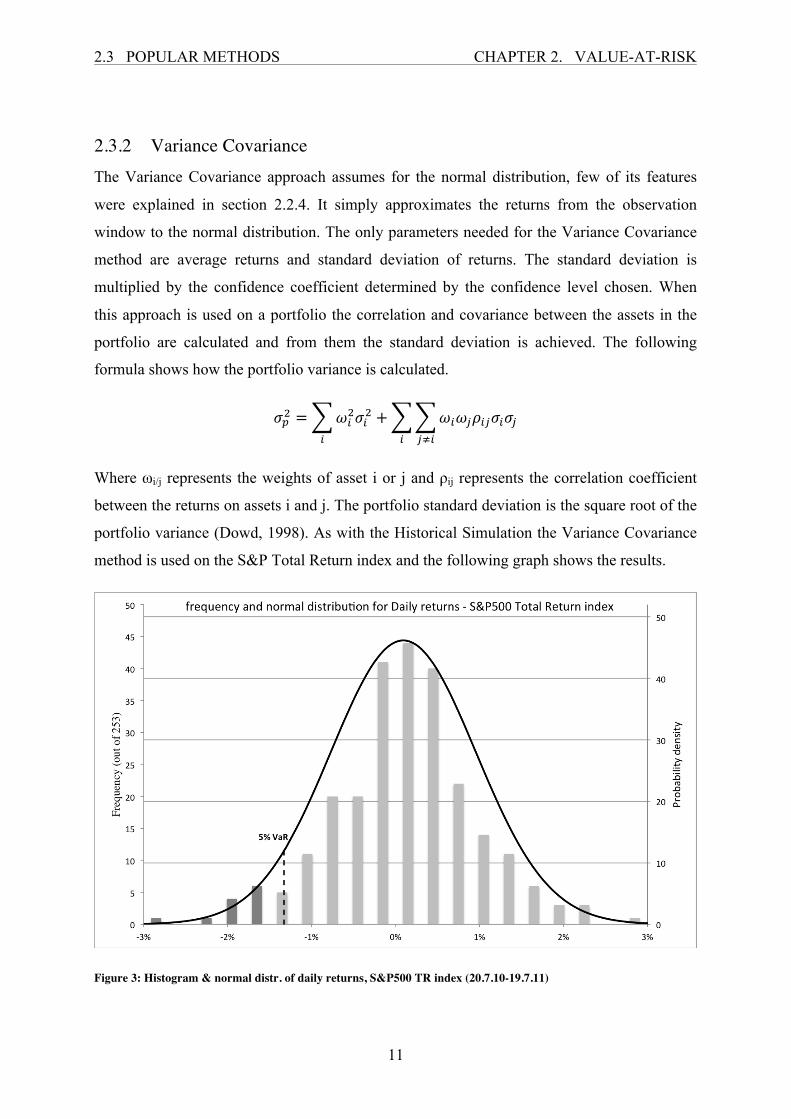
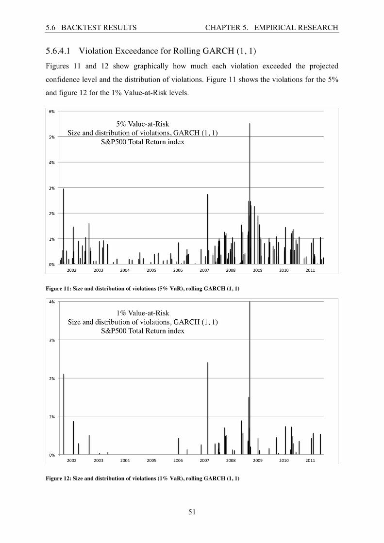
5.6.4.1 Violation Exceedance for Rolling GARCH (1, 1) Figures 11 and 12 show graphically how much each violation exceeded the projected

confidence level and the distribution of violations. Figure 11 shows the violations for the 5%

and figure 12 for the 1% Value-at-Risk levels.

Figure 11: Size and distribution of violations (5% VaR), rolling GARCH (1, 1)

Figure 12: Size and distribution of violations (1% VaR), rolling GARCH (1, 1)

5.6 BACKTEST RESULTS CHAPTER 5. EMPIRICAL RESEARCH

52

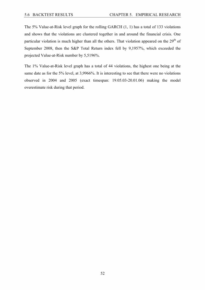
The 5% Value-at-Risk level graph for the rolling GARCH (1, 1) has a total of 133 violations

and shows that the violations are clustered together in and around the financial crisis. One

particular violation is much higher than all the others. That violation appeared on the 29th of

September 2008, then the S&P Total Return index fell by 9,1957%, which exceeded the

projected Value-at-Risk number by 5,5196%.

The 1% Value-at-Risk level graph has a total of 44 violations, the highest one being at the

same date as for the 5% level, at 3,9966%. It is interesting to see that there were no violations

observed in 2004 and 2005 (exact timespan: 19.05.03-20.01.06) making the model

overestimate risk during that period.

5.6 BACKTEST RESULTS CHAPTER 5. EMPIRICAL RESEARCH

53

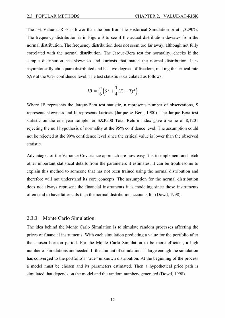
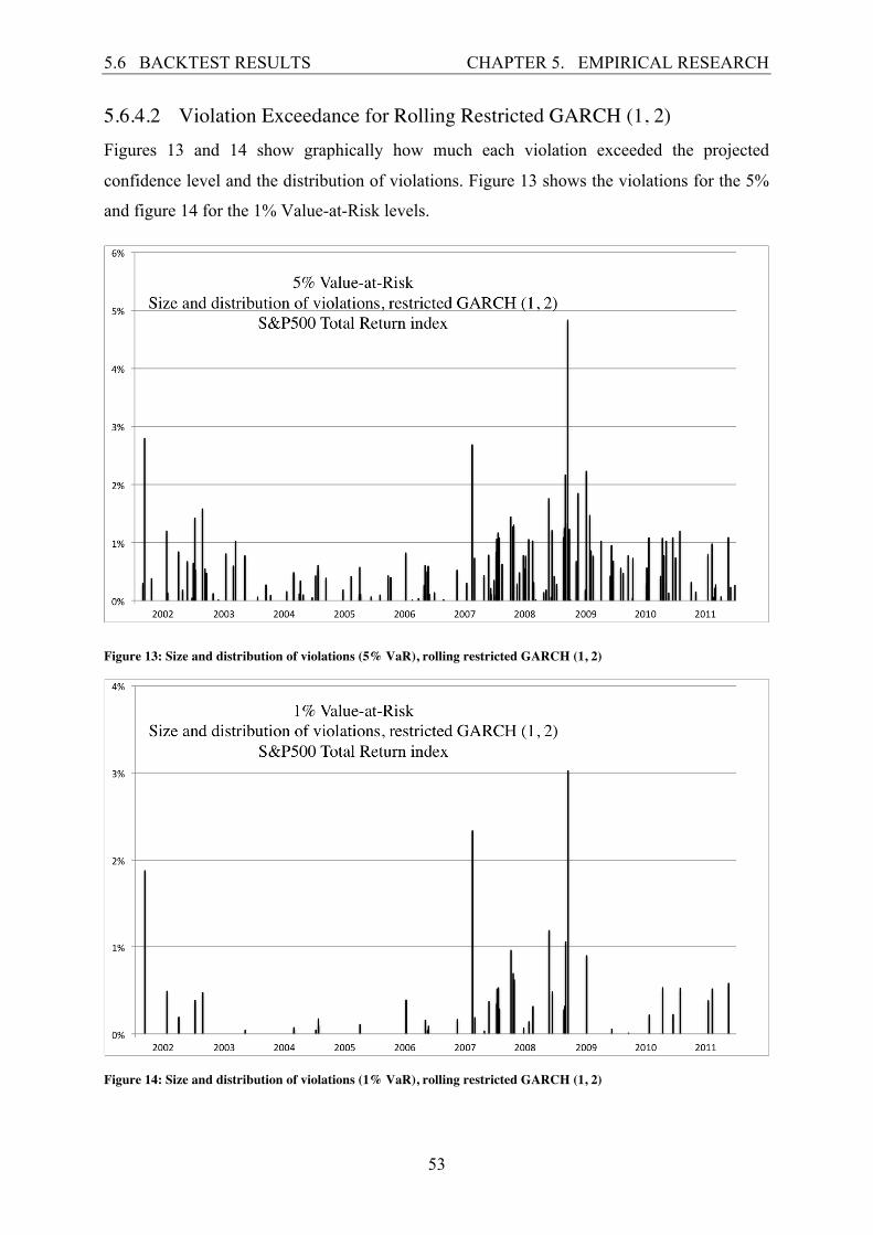
5.6.4.2 Violation Exceedance for Rolling Restricted GARCH (1, 2) Figures 13 and 14 show graphically how much each violation exceeded the projected

confidence level and the distribution of violations. Figure 13 shows the violations for the 5%

and figure 14 for the 1% Value-at-Risk levels.

Figure 13: Size and distribution of violations (5% VaR), rolling restricted GARCH (1, 2)

Figure 14: Size and distribution of violations (1% VaR), rolling restricted GARCH (1, 2)

5.6 BACKTEST RESULTS CHAPTER 5. EMPIRICAL RESEARCH

54

The 5% Value-at-Risk level graph for the rolling GARCH (1, 1) shows no striking difference

when it is compared to the graph for the rolling restricted GARCH (1, 2) model. The

violations are clustered in and around the financial crisis in both cases three exceedances are

highest at the same dates. The rolling restricted GARCH (1, 2) has 137 violations. The

highest exceedance is 4,8309% above the projected Value-at-Risk number. It does have lower

exceedances than the rolling GARCH (1, 1) as the Lopez’s loss function suggested.

The 1% Value-at-Risk level graph has a total of 47 violations, the highest exceedance is at

3,0225% and the exceedances are lower than for the rolling GARCH (1, 1) model. Violations

are observed in 2004 and 2005 making it not overestimate the risk during that period as much

the rolling GARCH (1, 1) did.

5.6 BACKTEST RESULTS CHAPTER 5. EMPIRICAL RESEARCH

55

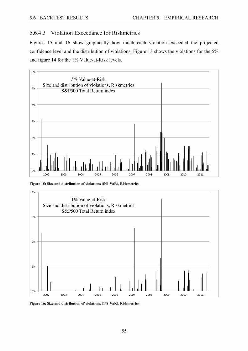
5.6.4.3 Violation Exceedance for Riskmetrics Figures 15 and 16 show graphically how much each violation exceeded the projected

confidence level and the distribution of violations. Figure 13 shows the violations for the 5%

and figure 14 for the 1% Value-at-Risk levels.

Figure 15: Size and distribution of violations (5% VaR), Riskmetrics

Figure 16: Size and distribution of violations (1% VaR), Riskmetrics

5.6 BACKTEST RESULTS CHAPTER 5. EMPIRICAL RESEARCH

56

The 5% Value-at-Risk level graph for the Riskmetrics model is similar, violations are

clustered together in and around the financial crisis and three of the highest exceedances are

at the same dates as with the other two models. The highest exceedance is at 5,3241% and

there are a total of 146 violations.

The 1% Value-at-Risk level graph has a total of 48 violations, the highest exceedance is at

3,7201%. There is a period of around one and a half year (11.04.02-24.09.03) where no

violations are observed, during which risk is overestimated.

All the models show similar patterns of distribution of violations and sizes at the 5% Value-

at-Risk level. At the 1% Value-at-Risk level the rolling GARCH (1, 1) and the Riskmetrics

model overestimated risk during certain periods. It should not be surprising that all the models

show similar results for the period since all the models come from the same family of time-

series models, the GARCH family.

57

6 Discussion

It was interesting to discover that the restricted GARCH (1, 2) model performed best under

the model selection process, showing the lowest values for both the AIC and SBC. The

residuals from this model show no sign of autocorrelation or heteroskedasticity, where the

residuals from the GARCH (1, 1) model did. However, this did not lead to the restricted

GARCH (1, 2) model outperforming the GARCH (1, 1) model when they were evaluated

with the backtests. The reason might be that since the AIC and SBC check for the fitness of

the model for the whole distribution and the backtests check a part of the distribution, the

GARCH (1, 1) model was better fitting for the left tail of the distribution. The sample

included the financial crisis of late 2008 that could also have been a factor in why the

restricted GARCH (1, 2) had lower AIC and SBC results than the GARCH (1, 1). The

restricted GARCH (1, 2) did outperform the GARCH (1, 1) for the With Crisis sample

backtests.

It is evident that the models did not perform well for the 1% Value-at-Risk level, this can be

due to the frequently observed fat tails in actual distribution of financial time-series and that

the normal assumption does not take account for those fat tails. Another distribution can be

used and compared with the normal distribution to see if it performs better at the 1% Value-

at-Risk level. The reason is likely that the conditional variance was abnormally high during

the financial crisis and therefore the absolute value of returns was high as well. Making the

negative returns surpass the 1% Value-at-Risk level more frequently.

It is problematic to find an optimal window size for GARCH models and different window

sizes show different estimates, this can be considered as a pitfall for studies when different

models are compared. Since it is relatively easy to manipulate data by changing window sizes

and show results that might be more fitting to the goals of the research.

To make an attempt to figure out why the restricted GARCH (1, 2) outperformed the GARCH

(1, 1) model in the model selection process. An assumption was made for the returns at time t

to be dependent on whether the returns are negative or positive at time t-1. The full sample

was split in two sub samples. One consisting of returns where the previous return had been

negative and the other consisting of returns where the previous return had been positive. The

preferred models were found from those sub-samples, according to the model selection

process and both sub-samples had the lowest AIC and SBC for the GARCH (1, 1) model.

CHAPTER 6. DISCUSSION

58

The residuals for the GARCH (1, 1) model of both sub-samples did not show any sign of

autocorrelation or heteroskedasticity either, with implementation of the Ljung-Box Q test and

the ARCH test. Then the GARCH variances were calculated for the time-series, where a

positive return used the estimates from the sub-sample consisting of returns with positive

previous returns and a negative return used the estimates from the other sub-sample. The

model estimated from both sub-samples was a rolling GARCH (1, 1) model with a window

size of 500. When the variances had been calculated the backtesting procedures were

performed and this model adjustment compared to the models used in the empirical research.

The model did not perform well enough according to the backtests and therefore the initial

assumption was weakened and the test statistics not included in the empirical research.

There is a vast amount of different models that can be tested, as the family of time-series

models only gets larger with time. It would be interesting to see results from other models.

59

7 Conclusion

The theoretical part of this thesis described how Value-at-Risk was developed and the

theories behind it. Fundamentals of the procedures were explained, the importance of marking

to market and the three parameters that needs to be specified for every model. Furthermore

BCBS and CESR regulations on how financial institutions should specify these parameters

were briefly described.

Known methods were described and applied to a part of the time-series to demonstrate the

differences between them.

Time-series analysis was introduced with explanation of tests that help examining the data.

The ICSS algorithm was explained and applied to find volatility change points. Furthermore

the ARCH (q) and GARCH (p, q) models were introduced and their properties.

The theories behind well known backtests, their differences and drawbacks are included in the

thesis.

The empirical research examines the ten year sample of S&P500 Total Returns index

(20.07.01-19.07.11) where a model selection process for the preferred GARCH (p, q) is

applied finding the restricted GARCH (1, 2) to be the best fit. The residuals from that model

along with the GARCH (1, 1) model were tested for serial autocorrelation and

heteroskedasticity, the results from these tests show evidence for autocorrelation and

heteroskedasticity in the residuals from the GARCH (1, 1) model while there is no evidence

of those factors in the residuals from the restricted GARCH (1, 2) models.

These models were given a rolling parameter estimation based on different window sizes and

they were backtested according to the tests described in the theoretical part. Eventually a

window size of 1500 was selected for the rolling GARCH (1, 1) and a window size of 500 for

the rolling restricted GARCH (1, 2). The Value-at-Risk estimates from these models were

used for evaluation against the Riskmetrics model. Where three samples were used: the entire

sample, before the financial crisis and with the financial crisis.

The results from the evaluation indicated that the rolling GARCH (1, 1) performed best for

the Full sample, the Riskmetrics performed best for the Before Crisis sample and the rolling

GARCH (1, 2) performed best for the With Crisis sample.

CHAPTER 7. CONCLUSION

60

The Lopez loss function was applied on the models used for the evaluation and resulting in

the rolling restricted GARCH (1, 2) showing the lowest value, the loss function calculates the

average exceedance level, which is contributed to when there is a violation. Along with the

results from the loss function, exceedance graphs with distribution of violations for all the

models at 5% and 1% Value-at-Risk levels were shown. They were similar for all the models

at the 5% level, however the 1% level showed that for certain periods both the rolling

GARCH (1, 1) and the Riskmetrics model had no violations, resulting in overestimation of

the risk.

61

8 Bibliography

Basel Committee on Banking Supervision. (2011, February). Revision to the Basel II market

risk framework. Basel, Switzerland.

Bollerslev, T. (1986). Generalized Autoregressive Conditional Heteroskedasticity. Journal of

Econometrics , 307-327.

Campbell, S. D. (2005, April 20). A Review of Backtesting and Backtesting Procedures.

Washington, D.C., US.

Christoffersen, P., & Pelletier, D. (2004). Backtesting Value-at-Risk: A Duration-Based

Approach. Journal of Financial Econometrics , 84-108.

Committee of European Securities Regulators. (2010, July 28). CESR's Guidelines on Risk

Measurement and the Calculation of Global Exposure and Counterparty Risk for UCITS.

Paris, France.

Croce, R. (2009, June 2). Primer on the Use of Geometric Brownian Motion in Finance.

Enders, W. (1995). Applied Econometric Time Series. Ames, Iowa: John Wiley & Sons.

Engle, R. F. (1982). Autoregressive Conditional Heteroscedasticity with Estimates of the

Variance of United Kingdom Inflation. Econometrica , 987-1008.

Engle, R. (2001). GARCH 101: The Use of ARCH/GARCH Models in Applied Econometrics.

Journal of Economic Perspectives , 157-168.

Dowd, K. (1998). Beyond value at risk: the new science of risk management. Chichester: John

Wiley & Sons Ltd.

Inclan, C., & Tiao, G. C. (1994). Use of Cumulative Sums of Squares for Retrospective

Detection of Changes of Variance. Journal of the American Statistical Association , 913-923.

Hamilton, D. J. (1994). Time Series Analysis. New Jersey: Princeton University Press.

Jarque, C. M., & Bera, A. K. (1980). Efficient Tests for Normality, Homoscedasticity and

Serial Independence of Regression Residuals. Economics Letters , 255-259.

Jorion, P. (2007). Value at Risk: The New Benchmark for Managing Financial Risk (3rd ed.).

New York: McGraw-Hill.

CHAPTER 8. BIBLIOGRAPHY

62

Ljung, G. M., & Box, G. E. (1978). On a measure of lack of fit in time series models.

Biometrika , 297-303.

Lopez, A. J. (1999). Methods for Evaluating Value-at-Risk Estimates. FRBSF Economic

Review , 3-17.

Néri, B. d. (2005, October 12). Backtesting Value-at-Risk Methodologies. Rio de Janeiro,

Brazil.

Nieppola, O. (2009). Backtesting Value-at-Risk Models. Helsinki, Finland.

Mina, J., & Xiao, Y. J. (2001, April). Return to RiskMetrics: The Evolution of a Standard.

New York, US.

Rouah, F. D., & Vainberg, G. (2007). Option Pricing Models and Volatility Using Excel-VBA.

New Jersey: John Wiley & Sons.

Tsay, R. S. (2005). Analysis of Financial Time Series (2nd ed.). New Jersey: John Wiley &

Sons.

63

9 Appendix A: VBA Codes

The codes are all designed for the VBA module to be set at

Option  Base  1  

It needs to be written at the start of the module.

When the results are given in arrays you need to press CMD + SHIFT + ENTER if you are

using a mac and CTRL + SHIFT + ENTER if you are using a pc. All the codes are fully

functional in the worksheets where they were applied found on the enclosed CD. To view

them you click the Developer tab in Excel and in there you click on Editor, then the relevant

module is selected. All the codes were created by the author except for the Nelder-Mead

algorithm attained from the enclosed CD from Rouah, F. D., & Vainberg, G. (2007).

Following are the codes used in this research.

9.1 ICSS Algorithm To use this code you need to select the cells where the results should appear (they appear as

an array, the size of it depending on the number of iterations and change points found). Then

write: “=ICSSalgorithm([insert selected range])” in the formula tab. The selected range

should be the returns data, which you are testing for, sorted by the most recent return at the

top of the range. It gives results as numbers, 1 representing the bottom observation, 2

representing the observation above etc. Each column carrying the results represents iteration

and the change points found during that iteration, 1st column being the first iteration, 2nd

column the second iteration etc. The code is as follows:

Function  ICSSalgorithm(returns  As  Range)    Dim  rflipped()  As  Variant    Dim  T  Dim  M  Dim  start  Dim  a  Dim  i  Dim  j  Dim  k  Dim  middle    a  =  1  

9.1 ICSS ALGORITHM CHAPTER 9. APPENDIX A: VBA CODES

64

start  =  1  T  =  returns.Rows.count  M  =  returns.Rows.count    Dim  count()  ReDim  count(M)    Dim  count2()  ReDim  count2(M)    ReDim  rflipped(M)  Dim  rflipped2()    Dim  c()  ReDim  c(T)    Dim  x()  ReDim  x(T)                    For  i  =  1  To  T                  rflipped(i)  =  returns.Cells(T  -­‐  (i  -­‐  1))          Next  i                    Dim  Tlast  Tlast  =  M  Dim  Tfirst  Tfirst  =  0  Dim  Tupper  Tupper  =  M            Dim  returnarray()  ReDim  returnarray(21,  50)    j  =  1  Do    ReDim  rflipped2((T  -­‐  start)  +  1)          For  i  =  1  To  ((T  -­‐  start)  +  1)                  rflipped2(i)  =  rflipped(start  -­‐  1  +  i)          Next  i    ReDim  count((T  -­‐  start)  +  1)          For  i  =  1  To  ((T  -­‐  start)  +  1)                  If  i  =  1  Then                  count(i)  =  1                  Else                  count(i)  =  1  +  count(i  -­‐  1)                  End  If          Next  i            ReDim  count2((T  -­‐  start)  +  1)          For  i  =  1  To  ((T  -­‐  start)  +  1)                  If  i  =  1  Then                  count2(i)  =  start                  Else                  count2(i)  =  1  +  count2(i  -­‐  1)                  End  If          Next  i            ReDim  c((T  -­‐  start)  +  1)          For  i  =  1  To  ((T  -­‐  start)  +  1)                  If  i  =  1  Then                  c(i)  =  rflipped2(i)  ^  2  

9.1 ICSS ALGORITHM CHAPTER 9. APPENDIX A: VBA CODES

65

               Else                  c(i)  =  rflipped2(i)  ^  2  +  c(i  -­‐  1)                  End  If          Next  i    ReDim  x((T  -­‐  start)  +  1)          For  i  =  1  To  ((T  -­‐  start)  +  1)                  x(i)  =  Abs(c(i)  /  c((T  -­‐  start)  +  1)  -­‐  i  /  ((T  -­‐  start)  +  1))          Next  i                      If  Sqr(((T  -­‐  start)  +  1)  /  2)  *  Application.Max(x)  >  1.358  And  (a  Mod  3  =  1)  Then          returnarray(1,  j)  =  Application.Index(count2,  Application.Match(Application.Max(x),  x,  0))          T  =  Application.Index(count,  Application.Match(Application.Max(x),  x,  0))  +  start  -­‐  1          Tupper  =  Application.Max(count)  +  start  -­‐  1          middle  =  T          a  =  a  +  1          Tfirst  =  T          Tlast  =  T          ElseIf  Sqr(((T  -­‐  start)  +  1)  /  2)  *  Application.Max(x)  <  1.358  And  (a  Mod  3  =  1)  Then          returnarray(1,  j)  =  0          a  =  a  +  1          start  =  T          ElseIf  Sqr(((T  -­‐  start)  +  1)  /  2)  *  Application.Max(x)  >  1.358  And  (a  Mod  3  =  2)  Then          returnarray(1,  j)  =  Application.Index(count2,  Application.Match(Application.Max(x),  x,  0))          T  =  Application.Index(count,  Application.Match(Application.Max(x),  x,  0))  +  start  -­‐  1          Tfirst  =  T          ElseIf  Sqr(((T  -­‐  start)  +  1)  /  2)  *  Application.Max(x)  <  1.358  And  (a  Mod  3  =  2)  Then          a  =  a  +  1          returnarray(1,  j)  =  0          start  =  middle  +  1          T  =  Tupper          ElseIf  Sqr(((T  -­‐  start)  +  1)  /  2)  *  Application.Max(x)  >  1.358  And  (a  Mod  3  =  0)  Then          returnarray(1,  j)  =  Application.Index(count2,  Application.Match(Application.Max(x),  x,  0))          start  =  Application.Index(count,  Application.Match(Application.Max(x),  x,  0))  +  start          Tlast  =  start  -­‐  1          ElseIf  Sqr(((T  -­‐  start)  +  1)  /  2)  *  Application.Max(x)  <  1.358  And  (a  Mod  3  =  0)  Then          a  =  a  +  1          returnarray(1,  j)  =  0          start  =  Tfirst  +  1          T  =  Tlast          End  If    j  =  j  +  1  Loop  Until  start  >  T  -­‐  2    Dim  temp  As  Variant    sorted  =  False  Do  While  Not  sorted  sorted  =  True  For  i  =  1  To  49          If  returnarray(1,  i)  >  returnarray(1,  i  +  1)  Then          temp  =  returnarray(1,  i  +  1)          returnarray(1,  i  +  1)  =  returnarray(1,  i)          returnarray(1,  i)  =  temp          sorted  =  False          End  If  Next  i  Loop    For  i  =  1  To  49          If  returnarray(1,  i)  =  returnarray(1,  i  +  1)  Then  

9.1 ICSS ALGORITHM CHAPTER 9. APPENDIX A: VBA CODES

66

       returnarray(1,  i)  =  0          End  If  Next  i    sorted  =  False  Do  While  Not  sorted  sorted  =  True  For  i  =  1  To  49          If  returnarray(1,  i)  >  returnarray(1,  i  +  1)  Then          temp  =  returnarray(1,  i  +  1)          returnarray(1,  i  +  1)  =  returnarray(1,  i)          returnarray(1,  i)  =  temp          sorted  =  False          End  If  Next  i  Loop    Do  While  returnarray(1,  1)  =  0  For  i  =  1  To  49          If  returnarray(1,  i)  =  0  Then          temp  =  returnarray(1,  i  +  1)          returnarray(1,  i  +  1)  =  returnarray(1,  i)          returnarray(1,  i)  =  temp          End  If  Next  i  Loop    Dim  NT  NT  =  0  Do  NT  =  NT  +  1  Loop  Until  returnarray(1,  NT)  =  0  NT  =  NT  -­‐  1    ReDim  Preserve  returnarray(21,  NT)    For  k  =  1  To  20  For  j  =  1  To  NT    If  j  =  1  And  (NT  >  1)  Then  start  =  1  T  =  returnarray(k,  j  +  1)  ElseIf  j  =  NT  And  (NT  >  1)  Then  start  =  returnarray(k,  j  -­‐  1)  +  1  T  =  M  ElseIf  j  =  1  And  (NT  =  1)  Then  start  =  1  T  =  M  Else  start  =  returnarray(k,  j  -­‐  1)  +  1  T  =  returnarray(k,  j  +  1)  End  If    ReDim  count((T  -­‐  start)  +  1)          For  i  =  1  To  ((T  -­‐  start)  +  1)                  If  i  =  1  Then                  count(i)  =  1                  Else                  count(i)  =  1  +  count(i  -­‐  1)                  End  If          Next  i            ReDim  rflipped2((T  -­‐  start)  +  1)  

9.1 ICSS ALGORITHM CHAPTER 9. APPENDIX A: VBA CODES

67

       For  i  =  1  To  ((T  -­‐  start)  +  1)                  rflipped2(i)  =  rflipped(start  -­‐  1  +  i)          Next  i    ReDim  c((T  -­‐  start)  +  1)          For  i  =  1  To  ((T  -­‐  start)  +  1)                  If  i  =  1  Then                  c(i)  =  rflipped2(i)  ^  2                  Else                  c(i)  =  rflipped2(i)  ^  2  +  c(i  -­‐  1)                  End  If          Next  i            ReDim  x((T  -­‐  start)  +  1)          For  i  =  1  To  ((T  -­‐  start)  +  1)                  x(i)  =  Abs(c(i)  /  c((T  -­‐  start)  +  1)  -­‐  i  /  ((T  -­‐  start)  +  1))          Next  i                    If  Sqr(((T  -­‐  start)  +  1)  /  2)  *  Application.Max(x)  >  1.358  And  (j  =  1)  Then          returnarray(k  +  1,  j)  =  Application.Index(count,  Application.Match(Application.Max(x),  x,  0))          ElseIf  Sqr(((T  -­‐  start)  +  1)  /  2)  *  Application.Max(x)  >  1.358  And  (j  >  1)  Then          returnarray(k  +  1,  j)  =  Application.Index(count,  Application.Match(Application.Max(x),  x,  0))  +  returnarray(k,  j  -­‐  1)          Else          returnarray(k  +  1,  j)  =  0          End  If    Next  j    sorted  =  False  Do  While  Not  sorted  sorted  =  True    For  i  =  1  To  NT  -­‐  1          If  returnarray(k  +  1,  i)  >  returnarray(k  +  1,  i  +  1)  Then          temp  =  returnarray(k  +  1,  i  +  1)          returnarray(k  +  1,  i  +  1)  =  returnarray(k  +  1,  i)          returnarray(k  +  1,  i)  =  temp          sorted  =  False          End  If  Next  i  Loop    For  i  =  1  To  NT  -­‐  1          If  returnarray(k  +  1,  i)  =  returnarray(k  +  1,  i  +  1)  Then          returnarray(k  +  1,  i)  =  0          End  If  Next  i    sorted  =  False  Do  While  Not  sorted  sorted  =  True    For  i  =  1  To  NT  -­‐  1          If  returnarray(k  +  1,  i)  >  returnarray(k  +  1,  i  +  1)  Then          temp  =  returnarray(k  +  1,  i  +  1)          returnarray(k  +  1,  i  +  1)  =  returnarray(k  +  1,  i)          returnarray(k  +  1,  i)  =  temp          sorted  =  False          End  If  Next  i  Loop    Do  While  returnarray(k  +  1,  1)  =  0  

9.1 ICSS ALGORITHM CHAPTER 9. APPENDIX A: VBA CODES

68

For  i  =  1  To  NT  -­‐  1          If  returnarray(k  +  1,  i)  =  0  Then          temp  =  returnarray(k  +  1,  i  +  1)          returnarray(k  +  1,  i  +  1)  =  returnarray(k  +  1,  i)          returnarray(k  +  1,  i)  =  temp          End  If  Next  i  Loop    For  i  =  1  To  NT          If  returnarray(k  +  1,  i)  =  0  Then          NT  =  0          Do          NT  =  NT  +  1          Loop  Until  returnarray(k  +  1,  NT)  =  0          NT  =  NT  -­‐  1          End  If  Next  i    Next  k    ICSSalgorithm  =  Application.Transpose(returnarray)    End  Function  

9.2 NELDER-MEAD ALGORITHM CHAPTER 9. APPENDIX A: VBA CODES

69

9.2 Nelder-Mead Algorithm To make the estimations for the GARCH (1, 1) model you select the cells where the results

should be in an array of four cells from top to bottom. And write: “=GARCHparams([insert

selected range],[insert range with estimation of parameters to start from])” in the formula bar.

The selected range should be the returns data, which you are estimating the parameters for,

sorted by the most recent return at the top of the range. The range with estimation of

parameters to start from, are specified values for omega, alpha and beta, where omega is at

the top and beta at the bottom. These values tell the algorithm at what value it should start the

process of finding the maximum log-likelihood. If they are very close to the actual values, the

parameter estimation process should not take as much computational time.

For the restricted GARCH (1, 2) model you do the same as with the GARCH (1, 1) except the

name of the function is GARCH12params, so write: “=GARCH12params([insert selected

range],[insert range with estimation of parameters to start from])” in the formula bar. The

specified values would then be for omega, alpha2 and beta. The code is as follows:

Function  BubSortRows(passVec)          Dim  tmpVec()  As  Double,  temp()  As  Double            uVec  =  passVec          rownum  =  UBound(uVec,  1)          colnum  =  UBound(uVec,  2)            ReDim  tmpVec(rownum,  colnum)  As  Double          ReDim  temp(colnum)  As  Double                      For  i  =  rownum  -­‐  1  To  1  Step  -­‐1                  For  j  =  1  To  i                          If  (uVec(j,  1)  >  uVec(j  +  1,  1))  Then                                  For  k  =  1  To  colnum                                          temp(k)  =  uVec(j  +  1,  k)                                          uVec(j  +  1,  k)  =  uVec(j,  k)                                          uVec(j,  k)  =  temp(k)                                  Next  k                          End  If                            Next  j          Next  i                    BubSortRows  =  uVec  End  Function      Function  NelderMead(fname  As  String,  rets,  startParams)          Dim  resMatrix()  As  Double          Dim  x1()  As  Double,  xn()  As  Double,  xw()  As  Double,  xbar()  As  Double,  xr()  As  Double,  xe()  As  Double,  xc()  As  Double,  xcc()          As  Double  

9.2 NELDER-MEAD ALGORITHM CHAPTER 9. APPENDIX A: VBA CODES

70

       Dim  funRes()  As  Double,  passParams()  As  Double          MAXFUN  =  1000          TOL  =  1e-­‐10          rho  =  1          Xi  =  2          gam  =  0.5          sigma  =  0.5                    paramnum  =  Application.Count(startParams)          ReDim  resmat(paramnum  +  1,  paramnum  +  1)  As  Double          ReDim  x1(paramnum)  As  Double,  xn(paramnum)  As  Double,  xw(paramnum)  As  Double,  xbar(paramnum)  As  Double,          xr(paramnum)  As  Double,  xe(paramnum)  As  Double,          xc(paramnum)  As  Double,  xcc(paramnum)  As  Double          ReDim  funRes(paramnum  +  1)  As  Double,  passParams(paramnum)          For  i  =  1  To  paramnum                  resmat(1,  i  +  1)  =  startParams(i)          Next  i          resmat(1,  1)  =  Run(fname,  rets,  startParams)                    For  j  =  1  To  paramnum                  For  i  =  1  To  paramnum                          If  (i  =  j)  Then                                  If  (startParams(i)  =  0)  Then                                          resmat(j  +  1,  i  +  1)  =  0.05                                  Else                                          resmat(j  +  1,  i  +  1)  =  startParams(i)  *  1.05                                  End  If                          Else                                  resmat(j  +  1,  i  +  1)  =  startParams(i)                          End  If                          passParams(i)  =  resmat(j  +  1,  i  +  1)                  Next  i                  resmat(j  +  1,  1)  =  Run(fname,  rets,  passParams)          Next  j                    For  lnum  =  1  To  MAXFUN                            resmat  =  BubSortRows(resmat)                  If  (Abs(resmat(1,  1)  -­‐  resmat(paramnum  +  1,  1))  <  TOL)  Then                          Exit  For                  End  If                                    f1  =  resmat(1,  1)                    For  i  =  1  To  paramnum                          x1(i)  =  resmat(1,  i  +  1)                  Next  i                  fn  =  resmat(paramnum,  1)                                    For  i  =  1  To  paramnum                          xn(i)  =  resmat(paramnum,  i  +  1)                  Next  i                  fw  =  resmat(paramnum  +  1,  1)                  For  i  =  1  To  paramnum                          xw(i)  =  resmat(paramnum  +  1,  i  +  1)                  Next  i                          For  i  =  1  To  paramnum                          xbar(i)  =  0                          For  j  =  1  To  paramnum                                  xbar(i)  =  xbar(i)  +  resmat(j,  i  +  1)                          Next  j                          xbar(i)  =  xbar(i)  /  paramnum  

9.2 NELDER-MEAD ALGORITHM CHAPTER 9. APPENDIX A: VBA CODES

71

               Next  i                                    For  i  =  1  To  paramnum                          xr(i)  =  xbar(i)  +  rho  *  (xbar(i)  -­‐  xw(i))                  Next  i                                    fr  =  Run(fname,  rets,  xr)                                    shrink  =  0                  If  ((fr  >=  f1)  And  (fr  <  fn))  Then                          newpoint  =  xr                          newf  =  fr                  ElseIf  (fr  <  f1)  Then                          'calculate  expansion  point                          For  i  =  1  To  paramnum                                  xe(i)  =  xbar(i)  +  Xi  *  (xr(i)  -­‐  xbar(i))                          Next  i                          fe  =  Run(fname,  rets,  xe)                          If  (fe  <  fr)  Then                                  newpoint  =  xe                                  newf  =  fe                          Else                                  newpoint  =  xr                                  newf  =  fr                          End  If                  ElseIf  (fr  >=  fn)  Then                          If  ((fr  >=  fn)  And  (fr  <  fw))  Then                                  For  i  =  1  To  paramnum                                          xc(i)  =  xbar(i)  +  gam  *  (xr(i)  -­‐  xbar(i))                                  Next  i                                  fc  =  Run(fname,  rets,  xc)                                  If  (fc  <=  fr)  Then                                          newpoint  =  xc                                          newf  =  fc                                  Else                                          shrink  =  1                                  End  If                          Else                                  For  i  =  1  To  paramnum                                          xcc(i)  =  xbar(i)  -­‐  gam  *  (xbar(i)  -­‐  xw(i))                                  Next  i                                  fcc  =  Run(fname,  rets,  xcc)                                  If  (fcc  <  fw)  Then                                          newpoint  =  xcc                                          newf  =  fcc                                  Else                                          shrink  =  1                                  End  If                          End  If                                    End  If                  If  (shrink  =  1)  Then                          For  scnt  =  2  To  paramnum  +  1                                  For  i  =  1  To  paramnum                                          resmat(scnt,  i  +  1)  =  x1(i)  +  sigma  *  (resmat(scnt,  i  +  1)  -­‐  x1(1))                                          passParams(i)  =  resmat(scnt,  i  +  1)                                  Next  i                                  resmat(scnt,  1)  =  Run(fname,  rets,  passParams)                          Next  scnt                  Else                          For  i  =  1  To  paramnum                                  resmat(paramnum  +  1,  i  +  1)  =  newpoint(i)                          Next  i  

9.2 NELDER-MEAD ALGORITHM CHAPTER 9. APPENDIX A: VBA CODES

72

                       resmat(paramnum  +  1,  1)  =  newf                  End  If                            Next  lnum          If  (lnum  =  MAXFUN  +  1)  Then                  MsgBox  "Maximum  Iteration  ("  &  MAXFUN  &  ")  exceeded"          End  If          resmat  =  BubSortRows(resmat)          For  i  =  1  To  paramnum  +  1                  funRes(i)  =  resmat(1,  i)          Next  i          funRes(1)  =  funRes(1)          NelderMead  =  Application.Transpose(funRes)            End  Function      Function  GARCHMLE(rets,  startParams)  Dim  VARt()  As  Double  n  =  Application.Count(rets)  ReDim  VARt(n)  As  Double  omega  =  startParams(1)  alpha  =  startParams(2)  beta  =  startParams(3)    If  ((omega  <  0)  Or  (alpha  <  0)  Or  (beta  <  0))  Or  (alpha  +  beta  >  0.99999)  Then          GARCHMLE  =  -­‐9999  Else    VARt(n)  =  Application.Var(rets)  GARCHMLE  =  -­‐Log(VARt(n))  -­‐  (rets(n)  ^  2  /  VARt(n))  For  cnt  =  n  -­‐  1  To  1  Step  -­‐1          VARt(cnt)  =  omega  +  alpha  *  rets(cnt  +  1)  ^  2  +  beta  *  VARt(cnt  +  1)          GARCHMLE  =  GARCHMLE  -­‐  Log(VARt(cnt))  -­‐  (rets(cnt)  ^  2  /  VARt(cnt))  Next  cnt  End  If          GARCHMLE  =  -­‐GARCHMLE  End  Function      Function  GARCHMLE12(rets,  startParams)  Dim  VARt()  As  Double  n  =  Application.Count(rets)  ReDim  VARt(n)  As  Double  omega  =  startParams(1)  alpha2  =  startParams(2)  beta  =  startParams(3)    If  ((omega  <  0)  Or  (alpha2  <  0)  Or  (beta  <  0))  Or  (alpha2  +  beta  >  0.99999)  Then          GARCHMLE12  =  -­‐9999  Else    VARt(n)  =  Application.Var(rets)  GARCHMLE12  =  -­‐Log(VARt(n))  -­‐  (rets(n)  ^  2  /  VARt(n))  For  cnt  =  n  -­‐  1  To  1  Step  -­‐1          VARt(cnt)  =  omega  +  alpha2  *  rets(cnt  +  2)  ^  2  +  beta  *  VARt(cnt  +  1)          GARCHMLE12  =  GARCHMLE12  -­‐  Log(VARt(cnt))  -­‐  (rets(cnt)  ^  2  /  VARt(cnt))  Next  cnt  End  If          GARCHMLE12  =  -­‐GARCHMLE12  End  Function      

9.2 NELDER-MEAD ALGORITHM CHAPTER 9. APPENDIX A: VBA CODES

73

Function  GARCHparams(rets,  startParams)          GARCHparams  =  NelderMead("GARCHMLE",  rets,  startParams)  End  Function      Function  GARCH12params(rets,  startParams)          GARCH12params  =  NelderMead("GARCHMLE12",  rets,  startParams)  End  Function  

9.3 VARIANCE FORECASTS CHAPTER 9. APPENDIX A: VBA CODES

74

9.3 Variance Forecasts To make a forecast for the variance from GARCH (1, 1) models you select a cell and write:

“=GARCHVarForecast([insert selected range], [insert omega value], [insert alpha value],

[insert beta value])” in the formula bar. The selected range should be the returns data, which

you are forecasting the next period variance for, sorted by the most recent return at the top of

the range. The omega, alpha and beta values are the estimated values of the parameters from

the GARCH (1, 1) model.

To make a forecast for the variance from restricted GARCH (1, 2) models you select a cell

and write: “=GARCH12VarForecast([insert selected range], [insert omega value], [insert

alpha2 value], [insert beta value])” in the formula bar. The selected range should be the

returns data, which you are forecasting the next period variance for, sorted by the most recent

return at the top of the range. The omega, alpha2 and beta values are the estimated values of

the parameters from the restricted GARCH (1, 2) model.

To make a forecast for the variance from Riskmetrics models you select a cell and write:

“=riskmetricVariance([insert selected range], [insert lambda value]” in the formula bar. The

selected range should be the returns data, which you are forecasting the next period variance

for, sorted by the most recent return at the top of the range. The lambda value is the chosen

lambda value for the forecast. The code is as follows:

Function  GARCHVarForecast(rng  As  Range,  omega  As  Double,  alpha  As  Double,  beta  As  Double)    Dim  flipped()  As  Variant    Dim  k  As  Integer  Dim  i  As  Integer    Dim  n  Dim  x    n  =  rng.Rows.Count    ReDim  flipped(n)            For  k  =  1  To  n                          flipped(k)  =  rng.Cells(n  -­‐  (k  -­‐  1))          Next  k            ReDim  x(n  +  1)  As  Double    For  i  =  1  To  n  +  1          If  i  =  1  Then          x(i)  =  omega  

9.3 VARIANCE FORECASTS CHAPTER 9. APPENDIX A: VBA CODES

75

       Else          x(i)  =  omega  +  alpha  *  flipped(i  -­‐  1)  ^  2  +  beta  *  x(i  -­‐  1)          End  If  Next  i    GARCHVarForecast  =  x(n  +  1)    End  Function      Function  GARCH12VarForecast(rng  As  Range,  omega  As  Double,  alpha2  As  Double,  beta  As  Double)    Dim  flipped()  As  Variant    Dim  k  As  Integer  Dim  i  As  Integer    Dim  n  Dim  x    n  =  rng.Rows.Count    ReDim  flipped(n)            For  k  =  1  To  n                          flipped(k)  =  rng.Cells(n  -­‐  (k  -­‐  1))          Next  k            ReDim  x(n  +  1)  As  Double    For  i  =  1  To  n  +  1          If  i  =  1  Then          x(i)  =  omega          ElseIf  i  =  2  Then          x(i)  =  omega  +  beta  *  x(i  -­‐  1)          Else          x(i)  =  omega  +  alpha2  *  flipped(i  -­‐  2)  ^  2  +  beta  *  x(i  -­‐  1)          End  If  Next  i    GARCH12VarForecast  =  x(n  +  1)    End  Function      Function  riskmetricVariance(rng  As  Range,  lambda)    Dim  i  Dim  n    n  =  rng.Rows.Count    Dim  x()  ReDim  x(n)    For  i  =  1  To  n          x(i)  =  (1  -­‐  lambda)  *  lambda  ^  (i  -­‐  1)  *  rng.Rows(i)  ^  2  Next  i    riskmetricVariance  =  Application.Sum(x)    End  Function