COMPENDIUM - munin.uit.no

CHAPTER 3: Getting Hamaker coefficients with an amplitude-modulation AFM in tapping mode

Laboratory for Energy and NanoScience

COMPENDIUM

CHAPTER 3: Getting Hamaker coefficients with an AM AFM in tapping mode LENS COMPENDIUM

2

LENS: Laboratory for Energy and Nano Science

LENS COMPENDIUM Published July 2020 Authors: Chia Yun Lai1

Tuza Olukan1 Sergio Santos1,3 Matteo Chiesa1,2 Corresponding author: Chia Yun Lai - [email protected] Affiliations: 1. Department of Physics and Technology, UiT The Arctic University of Norway, Tromso,

Norway 2. Laboratory for Energy and NanoScience (LENS), Khalifa University of Science and

Technology, Masdar Campus, Abu Dhabi, UAE 3. Future Synthesis, Skien, Norway Design and layout: Maritsa Kissamitaki1


3


CONTENTS

Getting Hamaker coefficients with an amplitude-modulation AFM in tapping mode .... 3

Steps to collect the raw data to reconstruct force profiles ............................................ 4

Steps to process the raw data .......................................................................................... 7

What does the Hamaker mean?.......................................................................................9 Examples of Hamaker maps in bimodal AM AFM………………………………………………………12 Bibliography ............................................................................................................... 12

Getting Hamaker coefficients with an amplitude-modulation AFM in tapping mode

We demonstrate how to get Hamaker coefficients with an amplitude-modulation AFM operated

in standard tapping mode. The Hamaker coefficient is a physical parameter that provides


4


chemical information about the surface of samples. It is based or emerges from van der Waals

forces. We use a Cypher scanning probe microscope from Asylum Research to demonstrate the

method. The method is based on the research carried out at LENS during the 10s decade and

early 20s.

Brief introduction of Hamaker coefficient

Rapid chemical mapping of substances with nanoscale resolution has been a target of

nanotechnologists1-3. The broader community relies on probing and identifying chemical

substances via standard spectrometry methods that exploit electromagnetic radiation

generating footprints associated to a wavelength of the electromagnetic spectrum at which

resonance is observed4. The preference for such methods is based on robust and reproducible

quantification and parameterization in measurements achieved by standard spectroscopy

methodologies and the possibility to directly map a physically relevant parameter to chemical

substances. To advance nanotechnology or nanosciences, higher lateral resolution is often

mandatory5,6. While AFM methods offer the possibility to enhance lateral resolution to sub-nm

levels, quantification commonly requires very specialized equipment7, special environmental

conditions such as ultra-high vacuum1,3,8 or the use of atomically flat surfaces1. Here, we set to

map a parameter related to the sample’s chemical composition, i.e. the Hamaker coefficient H,

directly from the standard observables in bimodal AFM via the non-invasive non-contact mode

of operation whereby mechanical contact with the sample is avoided9-17.

Steps to collect the raw data to reconstruct force profiles


5


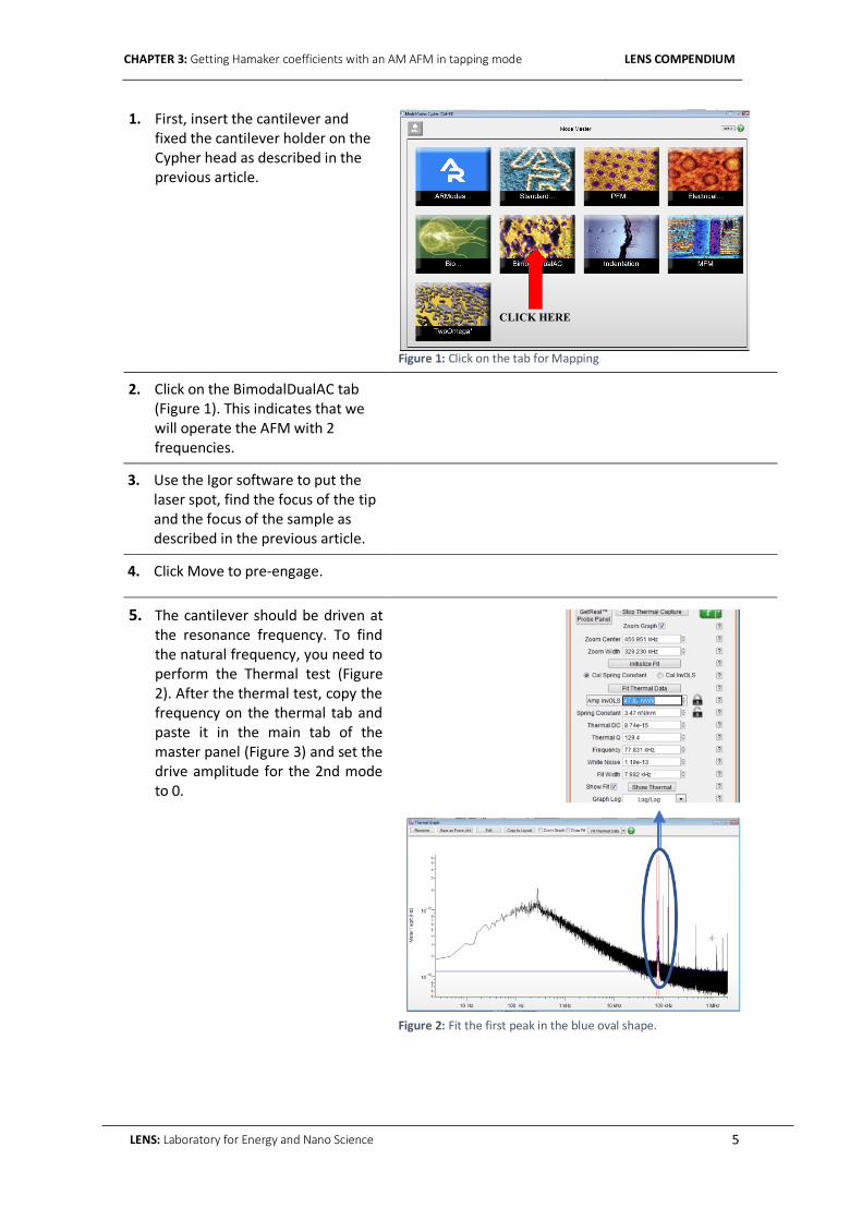
1. First, insert the cantilever and fixed the cantilever holder on the Cypher head as described in the previous article.

Figure 1: Click on the tab for Mapping

2. Click on the BimodalDualAC tab (Figure 1). This indicates that we will operate the AFM with 2 frequencies.

3. Use the Igor software to put the laser spot, find the focus of the tip and the focus of the sample as described in the previous article.

4. Click Move to pre-engage.

5. The cantilever should be driven at the resonance frequency. To find the natural frequency, you need to perform the Thermal test (Figure 2). After the thermal test, copy the frequency on the thermal tab and paste it in the main tab of the master panel (Figure 3) and set the drive amplitude for the 2nd mode to 0.

Figure 2: Fit the first peak in the blue oval shape.

CLICK HERE


6


Figure3: Paste the Thermal test result in the frequency field (red outline). Remember to set the amplitude for second mode (yellow outline) to 0.

6. Approach the tip in the same way as described in the previous article.

7. Perform a force-distance curve once while setting the force distance to 30 - 50 nm.

8. Perform the Thermal test again. After the thermal test, calibrate the 2nd mode first: copy the frequency (the peak position should be around 6 times of the 1st mode) on the thermal tab and paste it in the main tab of the master panel (Figure 3). Divide the amplitude in volts reading by 3.473 and fit the peak again to get spring constant and Q.

9. Calibrate the 1st mode: fit the 1st mode peak in the spectrum and copy the frequency on the thermal tab and paste it in the main tab of the master panel (Figure 4). Set back to the original amplitude in volts reading and fit the peak again to get spring constant and Q.

Figure 1: Amp InvOLS during first calibration in red outline. Amp invOLS during second calibration (yellow outline) is derived by dividing value in red outline by 3.473.

10. Then, find the AC as discussed in the previous article.


7


11. Set the free amplitude to ~0.7-0.8 times of AC, and the set-point to ~ 0.7-0.8 times of the free amplitude for the 1st mode. For the 2nd mode, set the free amplitude to ~0.1 times of 1st mode free amplitude.

12. Set the phase lag in both channel to 90°.

13. Set the scan size, scan rate and gain, and start scanning.

Steps to process the raw data

Note: R studio needs to be installed and add to the path. All the source codes can be found here

1. Copy the IBW files into the

UNPACKIGOR_2015APRIL_ImgBi folder and run the Matlab file: Unpack_BIMODAL_SASS_2016feb29 (Figure 5).

Figure 2: Copy your saved image in ".ibw" format into the specified directory.

2. NEW_TXT folder will be generated

when the code finishes running and renames the folder if needed (Figure 6).

Figure 3: Results of the extraction can be found in the "NEW_TXT" folder.

AFM RAW DATA((Your_RAWDATA_FILE).ibw) UNPACKIGOR_2015APRIL_ImgBi


8


3. Copy the 5 files (without def txt file) in the NEW_TXT folder into BIMODALHAMAKER_CloseForm\ DATA_images folder and run the Matlab file: Bimodal_Theory_2015Dec15 (Figure 7).

Figure 4: Copy all text files extracted from the raw data except the "Def.ibw".

4. Revise the parameters used in each experiment in the script (Figure 8).

Figure 5: Insert parameters obtained during the calibration stage in the parameter panel.

5. BIMODALHAMAKER_CloseForm\DA

TA _images\ProcessedData folder will be generated when the code finishes running (Figure 9).

Figure 6: Results are generated in the "ProcessedData" folder.

A1.txtA2.txtDef.txtH.txtP1.txtP2.txt

NEW_TXT DATA_images

BIMODALHAMAKER_CloseForm

k 1: Spring Constant first modeQ 1: Quality Factor first modef 1: Frequency first modek 2: Spring Constant second modeQ 2: Quality Factor second modeA01: Free Amplitude first modeA02: Free Amplitude second mode


9


What does the Hamaker mean? The Hamaker coefficient H, sometimes termed A outside the AFM community since in

AFM, A is reserved for amplitude, measures the strength between atoms due to van der

Waals forces. These forces are comparatively weak as compared to ionic and covalent

interactions. van der Waals (vdW) forces can refer to the London dispersion force

between atoms and sometimes also includes the Debye and Keesom interactions. A

standard book that covers these forces was written by J. Israelachvili18. This book is not

simple since it goes into the theory in quite detail. In Figure 10 as reproduced from Ref.

1919 the long-range forces acting between atoms on the surfaces of the tip and the

surface are illustrated in a). In b) the forces are illustrated for short range interactions

where mechanical contact occurs. Here the Hamaker coefficient and the respective

forces act as an adhesion force which is typically constant. The tip is modelled as a

sphere of radius R. A discussion of our models can be found in the papers above. In c)

we show the effective lateral resolution of both van der Waals, where the distance d

between the tip and the surface is larger than 0, and contact forces where d<0. We see

that the highest resolution would be achieved when very close to the surface. This is

because the long range vdW forces also induce lateral dispersion. In d) we show the

strength of the vdW interaction as parametrized by H and the effective area of

interaction with radius R.


10


Figure 10. a) Scheme of the non-contact interaction area Snc for a tip in the proximity of a surface for the long range attractive forces (d>a0). The tip radius is termed R. The gradient shows how the effective radius rnc grows as larger fractions p of the interaction are considered. This radius, and area, are thus termed rnc (p) and Snc (p) respectively. b) Scheme of effective radius ra (p) (attractive interactions) and rr (repulsive interactions) in the contact region where indentation occurs (d<a0). The effective value reff is a combination of rr and ra (p). c) Radius of interaction r versus distance d for ra/nc (p) (squares and rhombuses), rr (outlined circles) and reff (p) (triangles) for p=0.8 (red) and 0.9 (blue). Since ra (p) and rnc (p) are obtained from the same equations (Eqns. (1) and (2)) with the only difference being that for ra (p) d=a0, both are shown with the same markers as ra/nc (p) (squares and rhombuses). In the non-contact region, nc; reff (p)= ra/nc (p). d) Relationship between r and p for the long range interaction force. The vdW and DMT forces have been used to model the nc and c interaction areas throughout. A tip radius of 20 nm has been used to produce c) and d). All references in this caption refer to the paper “How localized are energy dissipation processes in the nanoscale?”


11


When water layers are present the distance d is affected by the height of the water

layers on the surfaces h. An example of this is shown in Figure 11 as reproduced from

Ref. 2020.

Figure 11. (a) Schematic representation of a cantilever probe interacting with a surface. L is the length of the probe in the vertical axis relative to the cantilever. This distance is typically of microscale dimensions and it is thus never used as a reference. (b) Schematic of the useful distances and separations for a tip interacting with the surface in dynamic AFM. Here, zc is the equilibrium tip−surface separation for the unperturbed cantilever where zc ≪ L. The instantaneous position of the tip relative to zc is z and d is the instantaneous tip−surface distance. (c) Schematic representation of the end of the tip with effective curvature R when both the tip and the surface are hydrated and covered by a layer of water of height h. The effective distance between the water on the tip and the water on the surface is d* where d* = d − 2h. (d) SEM image of the end of one of the sharp tips used in this work.

Examples of Hamaker maps in bimodal AM AFM


12


The first figures we published in 2016 on the mapping of the Hamaker coefficient while

simultaneously capturing the topography of the sample come from Ref. 16. In Figure 12

we have reproduced the most illustrative figure where we show the topography and the

derivative of the tip-sample force together with the Hamaker maps. These were

acquired simultaneously.

The top layer corresponds to a hydrophobic (1H,1H,2H,2H perfluorodecyl) acrylate

(PFDA) sample. The bottom layer corresponds to a calcite sample. The PFDA sample was

selected because it presents chemical heterogeneity in the 1-2 nm range. Heterogeneity

in van der Waals forces was thus demonstrated in the 1-2 nm lateral range and in the

10s of nm lateral range with the calcite sample.

Figure 12. Topography of (a) PFDA and (d) calcite obtained in bimodal AFM and corresponding (b) and (e) Fder and (c) and (f) Hamaker H.

The precursor of the theory of Hamaker reconstruction was written a few months before

in Ref. 2121. Anybody interested in the development of the theory can check the results

and discussion of this work.


13


Bibliography 1 Sugimoto, Y. et al. Chemical identification of individual surface atoms by atomic

force microscopy. Nature 446, 64-67 (2007). 2 Herruzo, E. T., Perrino, A. P. & Garcia, R. Fast nanomechanical spectroscopy of

soft matter. Nat Commun 5, 3126, doi:10.1038/ncomms4126 (2014). 3 Gross, L., Mohn, F., Moll, N., Liljeroth, P. & Meyer, G. The Chemical Structure of

a Molecule Resolved by Atomic Force Microscopy. Science 325, 1110-1114, doi:10.1126/science.1176210 (2009).

4 Banwell, C. N. & McCash, E. M. Fundamentals of molecular spectroscopy. Vol. 851 (McGraw-Hill New York, 1994).

5 Gross, L. et al. Organic structure determination using atomic-resolution scanning probe microscopy. Nat. Chem. 2, 821, doi:10.1038/nchem.765

https://www.nature.com/articles/nchem.765#supplementary-information (2010). 6 Hadlington, S. Nanostripe controversy in new twist,

<http://www.rsc.org/chemistryworld/2014/11/nanostripe-stripeynanoparticle-controversy-new-twist> (2014).

7 Sahin, O., Magonov, S., Su, C., Quate, C. F. & Solgaard, O. An atomic force microscope tip designed to measure time-varying nanomechanical forces. Nature nanotechnology 2, 507, doi:10.1038/nnano.2007.226

https://www.nature.com/articles/nnano.2007.226#supplementary-information (2007). 8 Setvín, M. et al. Chemical Identification of Single Atoms in Heterogeneous III–IV

Chains on Si(100) Surface by Means of nc-AFM and DFT Calculations. ACS nano 6, 6969-6976, doi:10.1021/nn301996k (2012).

9 Lai, C.-Y. et al. Explaining doping in material research (Hf substitution in ZnO films) by directly quantifying the van der Waals force. Physical Chemistry Chemical Physics 22, 4130-4137, doi:10.1039/C9CP06441A (2020).

10 Lu, J.-Y., Lai, C.-Y., Almansoori, I. & Chiesa, M. The evolution in graphitic surface wettability with first-principles quantum simulations: the counterintuitive role of water. Physical Chemistry Chemical Physics 20, 22636-22644, doi:10.1039/C8CP03633K (2018).

11 Liu, J., Lai, C.-Y., Zhang, Y.-Y., Chiesa, M. & Pantelides, S. T. Water wettability of graphene: interplay between the interfacial water structure and the electronic structure. RSC Advances 8, 16918-16926, doi:10.1039/C8RA03509A (2018).

12 Garlisi, C., Lai, C.-Y., George, L., Chiesa, M. & Palmisano, G. Relating Photoelectrochemistry and Wettability of Sputtered Cu- and N-Doped TiO2 Thin Films via an Integrated Approach. The Journal of Physical Chemistry C 122, 12369-12376, doi:10.1021/acs.jpcc.8b03650 (2018).

13 Chiou, Y.-C. et al. Direct Measurement of the Magnitude of the van der Waals Interaction of Single and Multilayer Graphene. Langmuir : the ACS journal of surfaces and colloids 34, 12335-12343, doi:10.1021/acs.langmuir.8b02802 (2018).

14 Santos, S., Lai, C.-Y., Olukan, T. & Chiesa, M. Multifrequency AFM: from origins to convergence. Nanoscale 9, 5038-5043, doi:10.1039/C7NR00993C (2017).


14


15 Lai, C.-Y., Santos, S. & Chiesa, M. Systematic Multidimensional Quantification of Nanoscale Systems From Bimodal Atomic Force Microscopy Data. ACS nano 10, 6265-6272, doi:10.1021/acsnano.6b02455 (2016).

16 Lai, C.-Y., Perri, S., Santos, S., Garcia, R. & Chiesa, M. Rapid quantitative chemical mapping of surfaces with sub-2nm resolution. Nanoscale, doi:10.1039/C6NR00496B (2016).

17 Garlisi, C., Scandura, G., Palmisano, G., Chiesa, M. & Lai, C.-Y. Integrated Nano- and Macroscale Investigation of Photoinduced Hydrophilicity in TiO2 Thin Films. Langmuir : the ACS journal of surfaces and colloids 32, 11813-11818, doi:10.1021/acs.langmuir.6b03756 (2016).

18 Israelachvili, J. Intermolecular & Surface Forces. 3 edn, (Academic Press, 2011). 19 Santos, S. et al. How localized are energy dissipation processes in nanoscale

interactions? Nanotechnology 22, 345401 (2011). 20 Santos, S., Stefancich, M., Hernandez, H., Chiesa, M. & Thomson, N. H.

Hydrophilicity of a Single DNA Molecule. The Journal of Physical Chemistry C 116, 2807-2818, doi:10.1021/jp211326c (2012).

21 Chia-Yun, L., Sergio, S. & Matteo, C. Reconstruction of height of sub-nanometer steps with bimodal atomic force microscopy. Nanotechnology 27, 075701 (2016).

Date post:	24-Mar-2022
Category:	Documents
Upload:	others
View:	2 times
Download:	0 times

COMPENDIUM - munin.uit.no

Documents