1

MM 416E ENERGY ENGINEERING COMPLEMENTARY NOTES

Prof. Dr. Şenol BAŞKAYA

PART-1 GENERAL CONCEPTS

Utilization Factors: Demand for electricity varies from hour to hour and from season to season. Depending on the energy demand and the economical conditions a power plant may be loaded at its full capacity or at partial load or shut down.

Time utilization factor: 8760

yearaintimeproductionActualFT =

Capacity Factor: capacityonInstallati

planttheofoutputPowerFC =

Load utilization factor: productionimumAnnual

productionActualFL max=

Reserve Calculations:

( ) teEtE μ.0= ⎥⎦⎤

⎢⎣⎡at ⎟⎟

⎠

⎞⎜⎜⎝

⎛+= 1ln1

0

0

ERtDμ

μ , tD: depletion time

Heating Value, Energy Released in Combustion:

⎥⎦

⎤⎢⎣

⎡−⎥⎦

⎤⎢⎣⎡ −

=Fkg

kJLHVs

FkgmQ FF &.

[ ]tkW

Heat Transferred to Working Fluid in Boiler:

BFB QQ η...

= where hB: Boiler efficiency TPP Efficiency:

F

elTPP

Q

P.=η

Annual Electricity Generation: ⎥⎦

⎤⎢⎣

⎡a

kWhel

[ ] [ ] ⎥⎦

⎤⎢⎣⎡−==ahFkWPAEGE LelIC 8760..

2

Annual Fuel Consumption:

[ ] ⎥⎦⎤

⎢⎣⎡=⎥⎦

⎤⎢⎣⎡−⎥⎦

⎤⎢⎣⎡=

at

ahF

htmAFC Lfuel 8760..&

⎥⎦⎤

⎢⎣⎡=

⎥⎦

⎤⎢⎣

⎡⋅⎥

⎦

⎤⎢⎣

⎡−

⎥⎦

⎤⎢⎣

⎡

=akg

kWhkWh

FkgkWh

H

akWh

AEGAFC

t

elTPP

tU

el

η

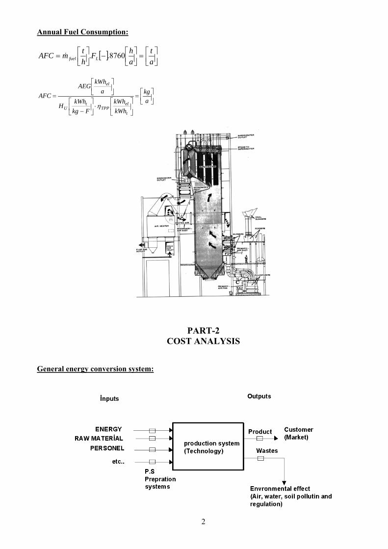
PART-2 COST ANALYSIS

General energy conversion system:

3

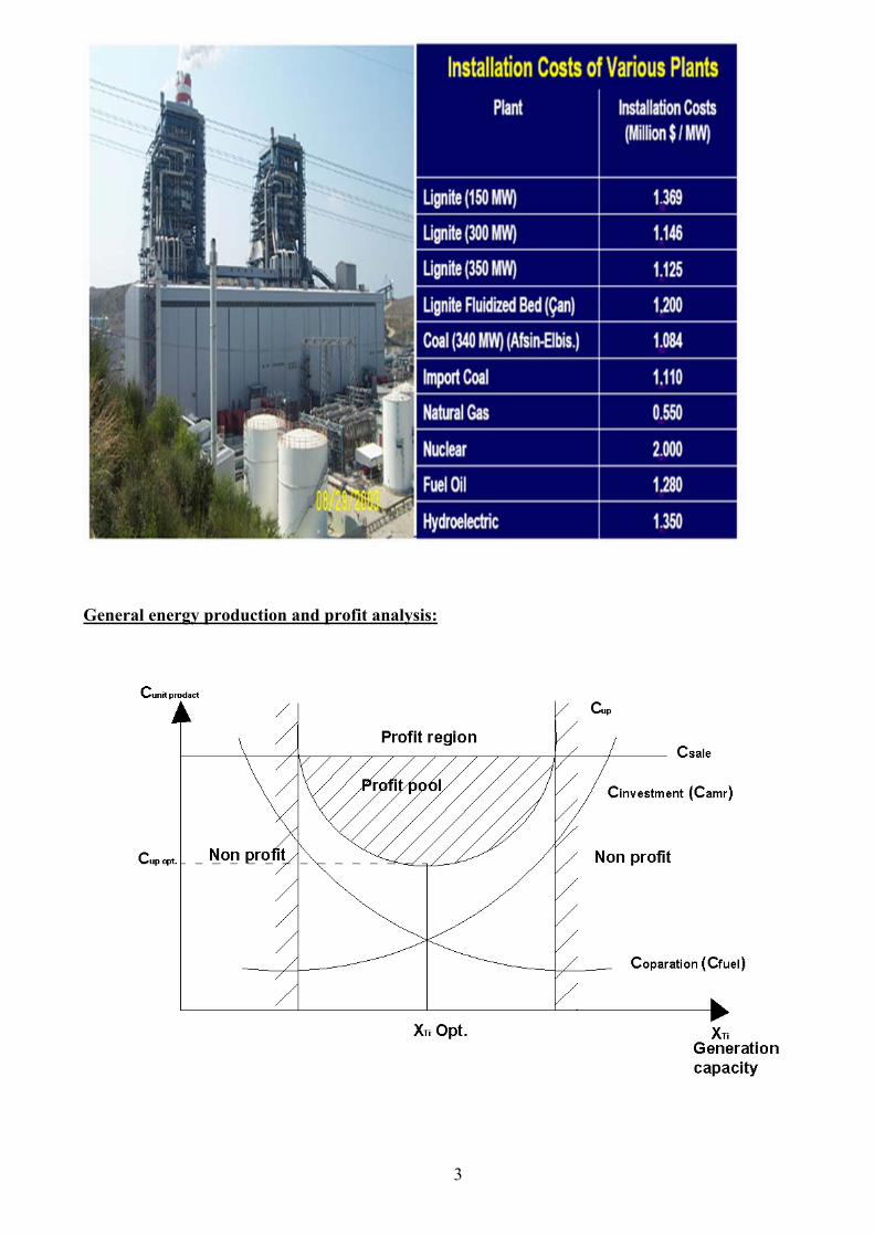
General energy production and profit analysis:

4

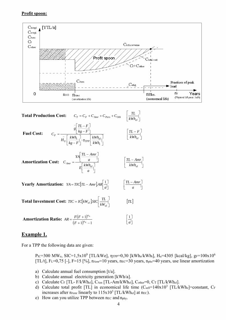
Profit spoon:

Total Production Cost: OthPersAmrFT CCCCC +++= ⎥⎦

⎤⎢⎣

⎡

elkWhTL

Fuel Cost: ⎥⎦

⎤⎢⎣

⎡⋅⎥⎦

⎤⎢⎣

⎡−

⎥⎦

⎤⎢⎣

⎡−−

=−

−

t

elTPP

tU

F

kWhkWh

FkgkWh

H

FkgFTLg

Cη

⎥⎦

⎤⎢⎣

⎡ −

elkWhFTL

Amortization Cost: ⎥⎦

⎤⎢⎣

⎡

⎥⎦⎤

⎢⎣⎡ −

=

akWh

E

aAmrTLYA

Cel

Amr ⎥⎦

⎤⎢⎣

⎡ −

elkWhAmrTL

Yearly Amortization: [ ] ⎥⎦

⎤⎢⎣⎡−=a

ARAmrTLTICYA 1. ⎥⎦⎤

⎢⎣⎡ −

aAmrTL

Total Investment Cost: [ ] ⎥⎦

⎤⎢⎣

⎡=

elel kW

TLSICkWICTIC . [ ]TL

Amortization Ratio: ( )( ) 11

1−+

+=

A

A

n

n

FFFAR ⎥⎦

⎤⎢⎣⎡a1

Example 1. For a TPP the following data are given:

PIC=300 MWe, SIC=1,5x109 [TL/kWe], ηTPP=0,30 [kWhe/kWht], Hu=4305 [kcal/kg], gF=100x106 [TL/t], FL=0,75 [-], F=15 [%], nAmr=10 years, nEC=30 years, nphs=40 years, use linear amortization

a) Calculate annual fuel consumption [t/a]. b) Calculate annual electricity generation [kWh/a]. c) Calculate CF [TL- F/kWhel], CAm [TL-Am/kWhel], Cother=0, CT [TL/kWhel]. d) Calculate total profit [TL] in economical life time (Csell=140x103 [TL/kWhe]=constant, CF

increases after nAmr linearly to 115x103 [TL/kWhel] at nEC). e) How can you utilize TPP between nEC and nphy.

5

Answer:

a) [ ] ⎥⎦⎤

⎢⎣⎡=⎥⎦

⎤⎢⎣⎡−⎥⎦

⎤⎢⎣⎡=

at

ahF

htMAFC LF 8760..

.

[ ][ ]−⎥

⎦

⎤⎢⎣

⎡−

=

TPPt

U

tICF

FkgkWhH

kWPMη.

.

= [ ]

⎥⎦

⎤⎢⎣

⎡⎥⎦

⎤⎢⎣

⎡− t

elt

e

kWhkWh

FkgkWh

kW

30,0861

4305000.300 = 200.000

hFkg − = 200

hFt −

[ ] ⎥⎦⎤

⎢⎣⎡ −

=⎥⎦⎤

⎢⎣⎡−⎥⎦

⎤⎢⎣⎡ −

=aFtx

ah

hFtAFC 6

.10314,18760.75,0.200

b) [ ] [ ] ⎥⎦⎤

⎢⎣⎡−=ahFkWPE LelIC 8760..

[ ] [ ] ⎥⎦⎤

⎢⎣⎡=⎥⎦

⎤⎢⎣⎡−=

akWhx

ahkWE e

e910971,18760.75,0.000.300

c) ⎥⎦

⎤⎢⎣

⎡ −=

⎥⎦

⎤⎢⎣

⎡⎥⎦

⎤⎢⎣

⎡−

⎥⎦

⎤⎢⎣

⎡−

=

⎥⎦

⎤⎢⎣

⎡⋅⎥⎦

⎤⎢⎣

⎡−

⎥⎦

⎤⎢⎣

⎡−−

=

−

e

t

et

t

elTPP

t

F

F kWhFTLx

kWhkWhx

FkgkWh

Fkgt

tTLx

kWhkWh

FkgkWhLHV

FkgFTLg

C 3

6

107,663,0

8614305

100010100

η

⎥⎦⎤

⎢⎣⎡

⎥⎦⎤

⎢⎣⎡ −

=

akWh

AEG

aAmrTLYA

Cel

Amr , TYxAOYA =

[ ]TLxkWTLxxkWxSICPTY

eeIC

129 10450105,1000.300 =⎥⎦

⎤⎢⎣

⎡==

( )( ) ⎥⎦

⎤⎢⎣⎡≅

−++

=−+

+=

aFFFAO

A

A

n

n 12,01)115,0(

)115,0(15,011

110

10

[ ] ⎥⎦⎤

⎢⎣⎡=⎥⎦

⎤⎢⎣⎡=

aTLx

axTLxYA 1212 109012,010450

⎥⎦

⎤⎢⎣

⎡ −=

⎥⎦⎤

⎢⎣⎡

⎥⎦⎤

⎢⎣⎡ −

=ee

Amr kWhAmrTLx

akWhx

aAmrTLx

C 3

9

12

107,4510971,1

1090

⎥⎦

⎤⎢⎣

⎡=+++=

eOthPersAmrFT kWh

TLxCCCCC 3104,112

6

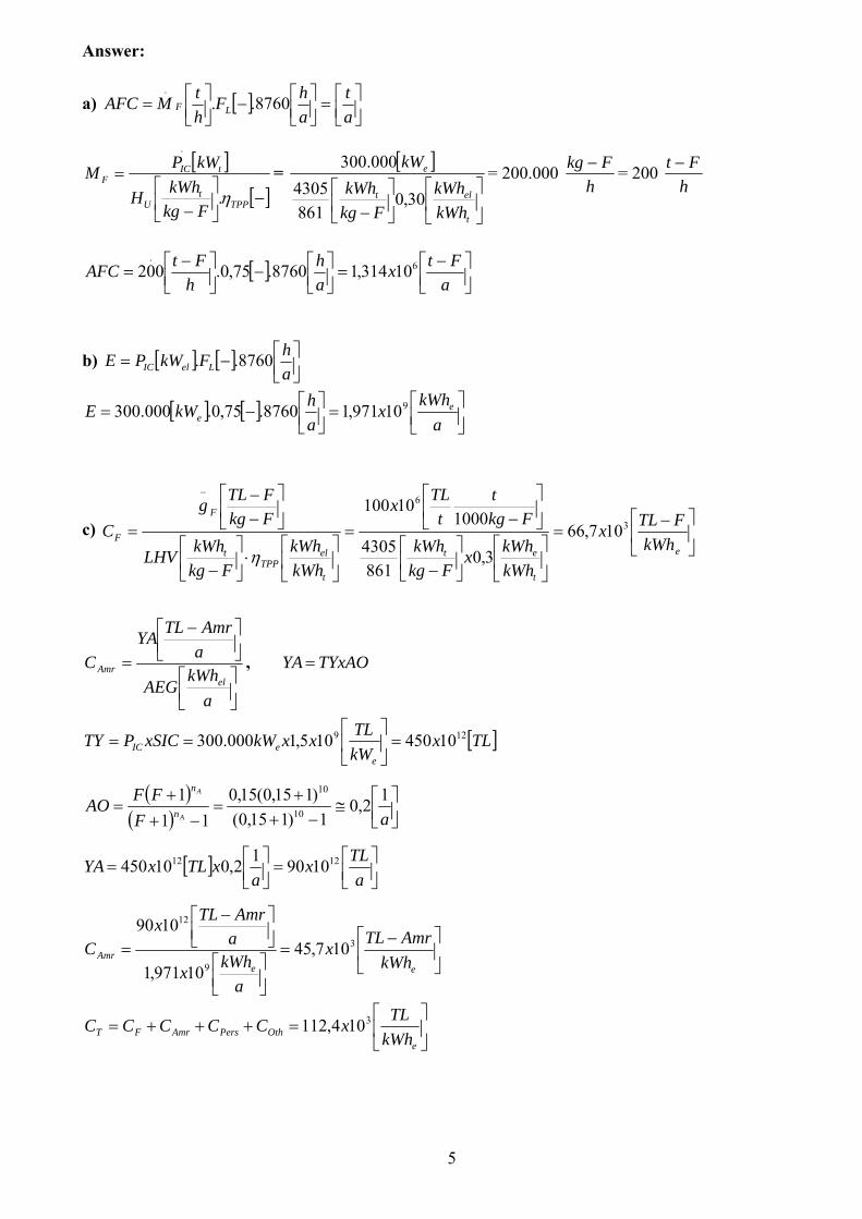
d)

[ ] [ ] [ ] [ ] [ ]TLxxxxxxaxna

kWhxEkWhTLCCC Amr

e

eTsellnprofit Amr

12933 105441010971,1104,11210140 =−=⎥⎦⎤

⎢⎣⎡

⎥⎦

⎤⎢⎣

⎡−=−

( ) ( )AmrECFF

Fsellnnofit nnxExCC

CCC nAmrnec

necECAmr−

⎥⎥⎦

⎤

⎢⎢⎣

⎡⎟⎟⎠

⎞⎜⎜⎝

⎛ −+−=−− 2Pr

( ) ( ) [ ]TLxxxxxxxxCECAmr nnofit

15933

33Pr 1094,1103010971,1

2107,66101151011510140 =−⎥

⎦

⎤⎢⎣

⎡⎟⎟⎠

⎞⎜⎜⎝

⎛ −+−=−−

[ ]TLxCCCECAmrAmr nnofitnofittotalofit

15PrPrPr 10484,2=+= −−−−

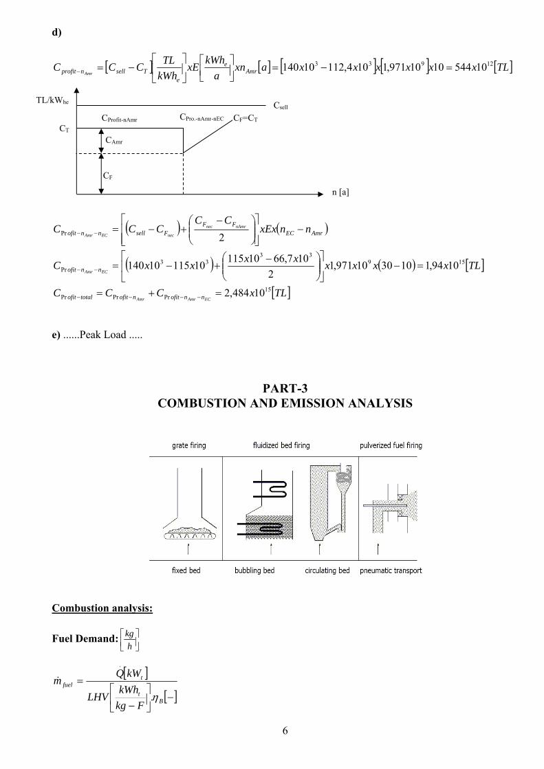
e) ......Peak Load .....

PART-3

COMBUSTION AND EMISSION ANALYSIS

Combustion analysis:

Fuel Demand: ⎥⎦⎤

⎢⎣⎡

hkg

[ ]

[ ]−⎥⎦

⎤⎢⎣

⎡−

=

Bt

tfuel

FkgkWh

LHV

kWQm

η.

.

&

TL/kWhe

n [a]

CF

CT CAmr

CProfit-nAmr CF=CT

Csell

CPro.-nAmr-nEC

7

[ ]

⎥⎦

⎤⎢⎣

⎡⎥⎦

⎤⎢⎣

⎡−

=

t

elPP

t

elelfuel

kWhkWh

FkgkWh

LHV

kWPm

η.&

Combustion Air Demand:

⎥⎦

⎤⎢⎣

⎡−−

∀⎥⎦⎤

⎢⎣⎡ −

=∀FkgANm

hFkgm afuela

3

.&& [Nm3-A/ h] ⎥⎦

⎤⎢⎣

⎡−−

∀=∀FkgANmn ata

3

. 221

21O

n−

=

Combustion Gas Flow:

⎥⎦

⎤⎢⎣

⎡−−

∀⎥⎦⎤

⎢⎣⎡ −

=∀ −−− FkgGNm

hFkgm wetDryfgfuelwetDryfg

3

.&& ⎥⎥⎦

⎤

⎢⎢⎣

⎡ −h

GNm3

( )

tawetdryfgtwetdryfg n ∀−+∀=∀ −−−− .1 , OHdryfgfg 2∀+∀=∀ −

)9(244.12 HOH mw +=∀ , [Nm3/kg fuel] solid and liquid fuels

)2

(22 nmHCHOH

n∀+∀=∀ , [Nm3/ Nm3fuel] gas fuels

273273.00

3 +∀=⎥

⎦

⎤⎢⎣

⎡∀ −−

Th

mCfgTfg

&&

8

Emission analysis:

Total Emission: ⎥⎥⎦

⎤

⎢⎢⎣

⎡ −∀

⎥⎥⎦

⎤

⎢⎢⎣

⎡

−−

= − hfgNm

fgNmpolkgm dry

dryfgdry

Mpol

3

3 .. && ε [kg-pol/h]

⎥⎦⎤

⎢⎣⎡ −

⎥⎦

⎤⎢⎣

⎡−−

= − hFuelkgm

fuelkgpolkgm fuelFMpol && .ε ⎥⎦

⎤⎢⎣⎡

⎥⎦

⎤⎢⎣

⎡ −= − h

kWhEG

kWhpolkgm el

elkWhMpol el

.ε&

Volume based Emission Factor: [ ]ppmfgNmEmNm

dryVV =

⎥⎥⎦

⎤

⎢⎢⎣

⎡

−−

−6

3

3

10ε

Mass Based Emission factor: kmol

kmoldry

VM VMppm

EmkmolEmNmV

EmkmolEmkgM

fgNmEmNm

633

3

10=

⎥⎦

⎤⎢⎣

⎡−−

⎥⎦⎤

⎢⎣⎡

−−

×⎥⎥⎦

⎤

⎢⎢⎣

⎡

−−

= εε ⎥⎥⎦

⎤

⎢⎢⎣

⎡

−−

dryfgNmEmkg

3

Fuel Related Emission Factor: [ ]

[ ] dryfg

kmolDry

FM

polkmolpolNmV

polkmolpolkgM

fgNmpolNmppm

−− ∀

⎥⎦

⎤⎢⎣

⎡

⎥⎦

⎤⎢⎣

⎡

−−

=

.

..

.

10 336

3

ε ⎥⎦

⎤⎢⎣

⎡−−

Fkgpolkg

Boiler Related Emission : [ ]−×⎥⎦

⎤⎢⎣

⎡ −×⎥⎦

⎤⎢⎣

⎡−−

= −−Bt

FMQM kWhFkg

LHVFkgpolkg

ηεε 11 ⎥

⎦

⎤⎢⎣

⎡ −

tkWhpolkg

Emission Emitted Per elkWh :PPt

FMElM kWhFkg

LHVFkgpolkg

ηεε 11

×⎥⎦

⎤⎢⎣

⎡ −×⎥

⎦

⎤⎢⎣

⎡−−

= −− ⎥⎦

⎤⎢⎣

⎡ −

elkWhpolkg

9

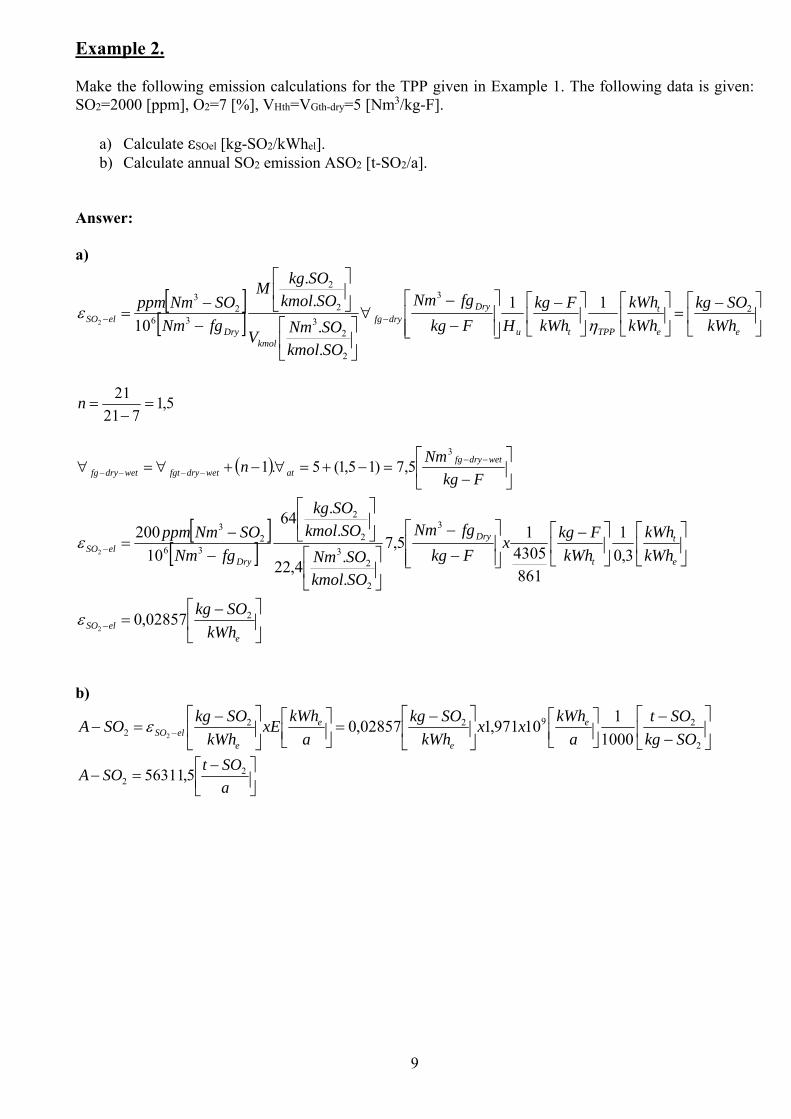
Example 2. Make the following emission calculations for the TPP given in Example 1. The following data is given: SO2=2000 [ppm], O2=7 [%], VHth=VGth-dry=5 [Nm3/kg-F].

a) Calculate εSOel [kg-SO2/kWhel]. b) Calculate annual SO2 emission ASO2 [t-SO2/a].

Answer: a)

[ ][ ] ⎥

⎦

⎤⎢⎣

⎡ −=⎥

⎦

⎤⎢⎣

⎡⎥⎦

⎤⎢⎣

⎡ −

⎥⎥⎦

⎤

⎢⎢⎣

⎡

−

−∀

⎥⎦

⎤⎢⎣

⎡

⎥⎦

⎤⎢⎣

⎡

−−

= −−ee

t

TPPtu

Drydryfg

kmolDry

elSO kWhSOkg

kWhkWh

kWhFkg

HFkgfgNm

SOkmolSONmV

SOkmolSOkgM

fgNmSONmppm 2

3

2

23

2

2

362

3 11

..

..

102 ηε

5,1721

21=

−=n

( ) ⎥⎦

⎤⎢⎣

⎡−

=−+=∀−+∀=∀ −−−−−− Fkg

Nmn wetdryfgatwetdryfgtwetdryfg

3

5,7)15,1(5.1

[ ][ ] ⎥

⎦

⎤⎢⎣

⎡⎥⎦

⎤⎢⎣

⎡ −

⎥⎥⎦

⎤

⎢⎢⎣

⎡

−

−

⎥⎦

⎤⎢⎣

⎡

⎥⎦

⎤⎢⎣

⎡

−−

=−e

t

t

Dry

DryelSO kWh

kWhkWh

FkgxFkgfgNm

SOkmolSONm

SOkmolSOkg

fgNmSONmppm

3,01

8614305

15,7

.

.4,22

..64

10200 3

2

23

2

2

362

3

2ε

⎥⎦

⎤⎢⎣

⎡ −=−

eelSO kWh

SOkg 202857,02

ε

b)

⎥⎦

⎤⎢⎣

⎡−−

⎥⎦⎤

⎢⎣⎡

⎥⎦

⎤⎢⎣

⎡ −=⎥⎦

⎤⎢⎣⎡

⎥⎦

⎤⎢⎣

⎡ −=− −

2

29222 1000

110971,102857,02 SOkg

SOta

kWhxxkWh

SOkga

kWhxEkWh

SOkgSOA e

e

e

eelSOε

⎥⎦⎤

⎢⎣⎡ −

=−aSOtSOA 2

2 5,56311

10

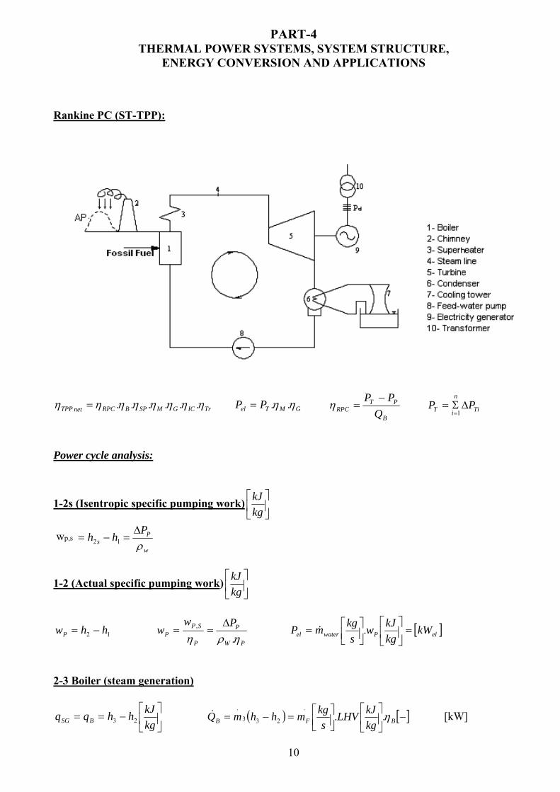
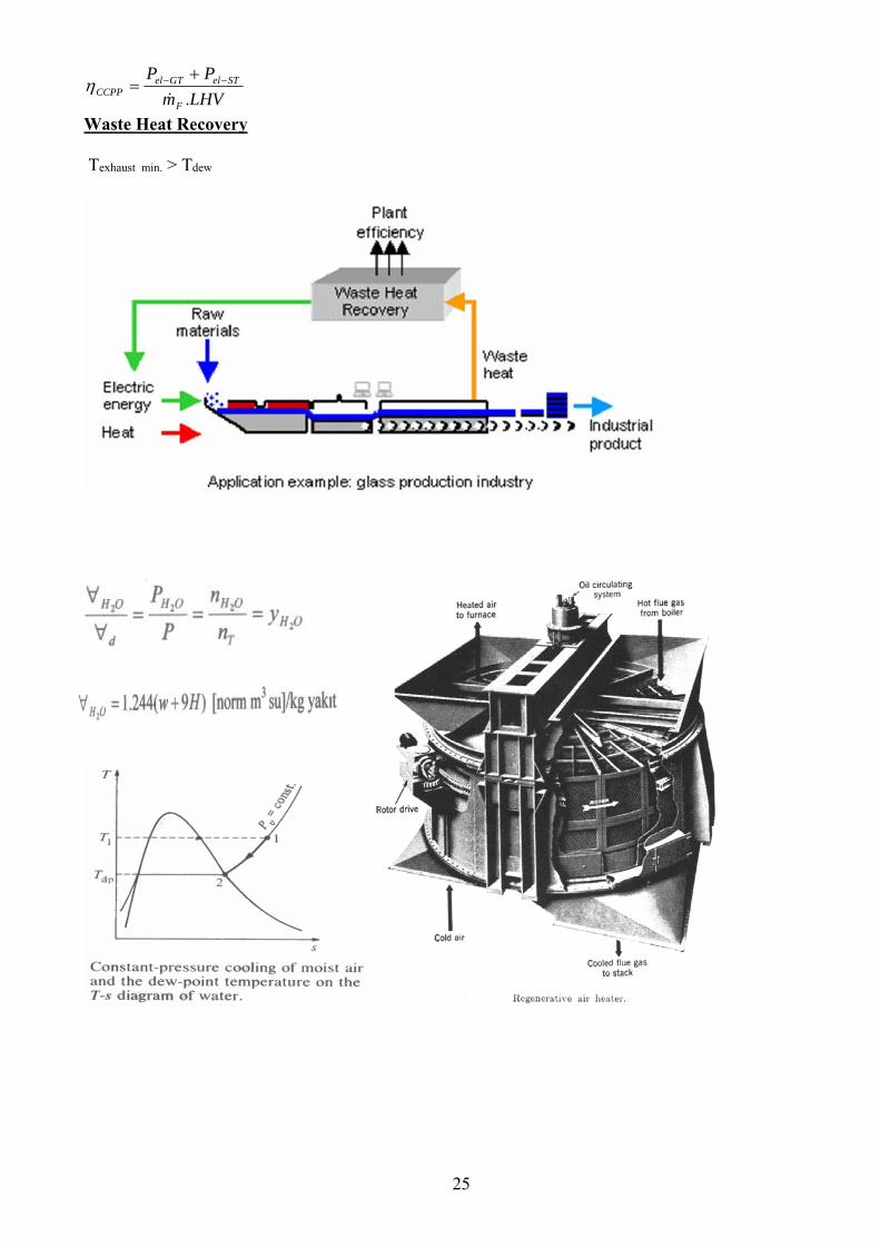
PART-4 THERMAL POWER SYSTEMS, SYSTEM STRUCTURE,

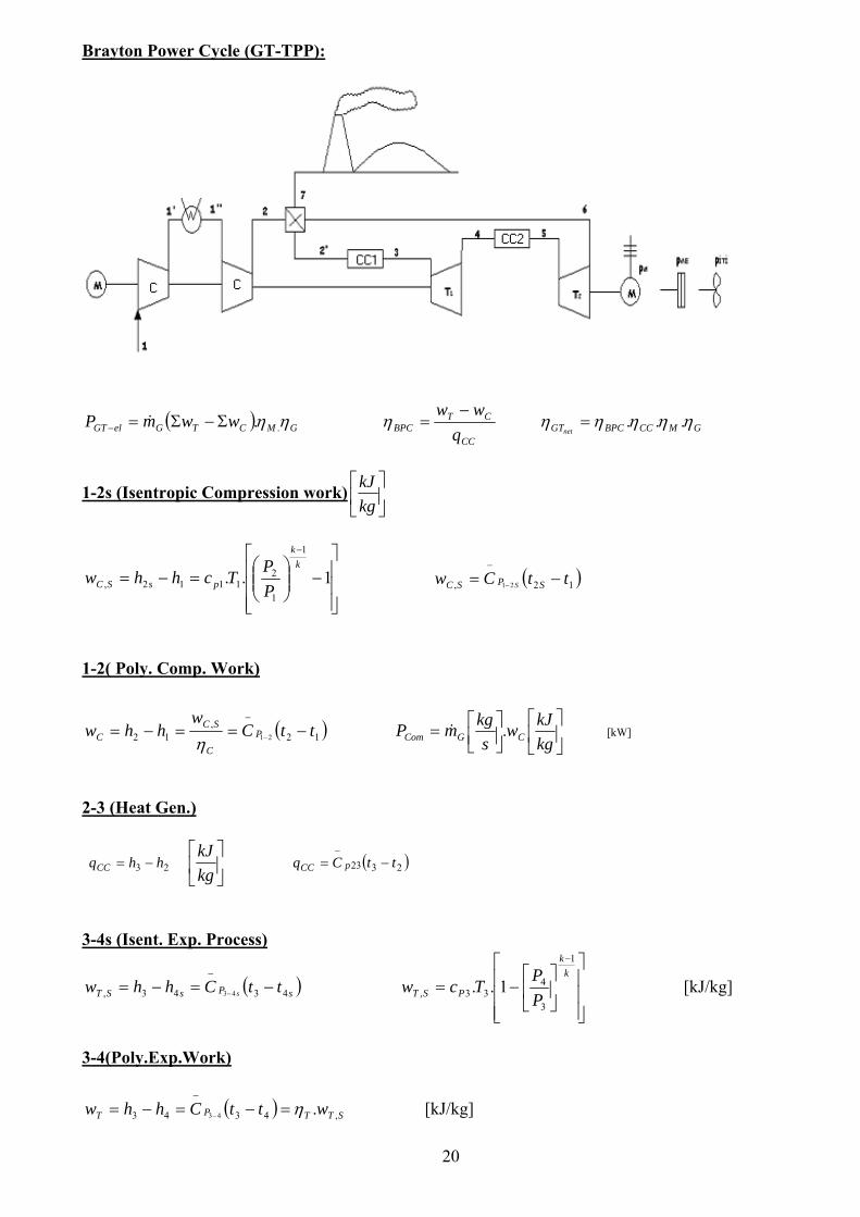
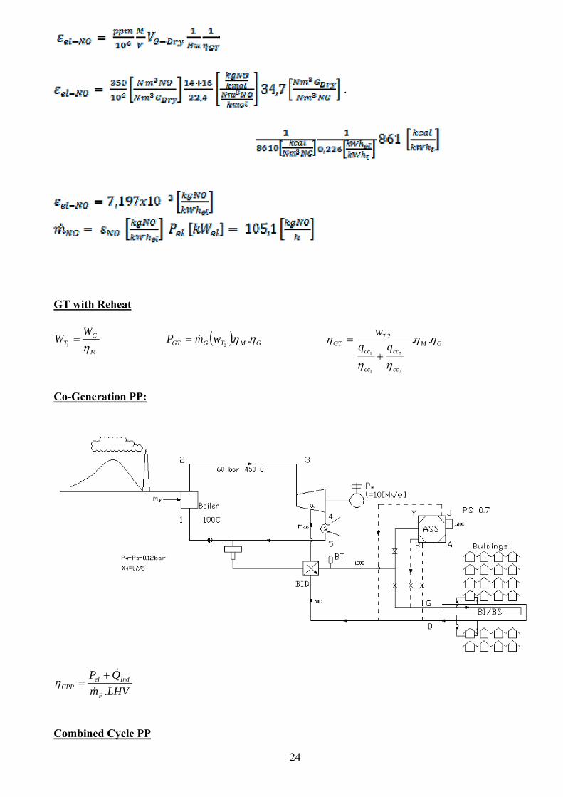
ENERGY CONVERSION AND APPLICATIONS Rankine PC (ST-TPP):

TrICGMSPBRPCnetTPP ηηηηηηηη ......= GMTel PP ηη ..= B

PTRPC Q

PP −=η Ti

n

iT PP ΔΣ==1

Power cycle analysis:

1-2s (Isentropic specific pumping work) ⎥⎦

⎤⎢⎣

⎡kgkJ

wp,s 12 hh s −=w

PPρΔ

=

1-2 (Actual specific pumping work) ⎥⎦

⎤⎢⎣

⎡kgkJ

12 hhwP −= PW

P

P

SPP

Pww

ηρη ., Δ== [ ]elPwaterel kW

kgkJw

skgmP =⎥

⎦

⎤⎢⎣

⎡⎥⎦⎤

⎢⎣⎡= .&

2-3 Boiler (steam generation)

⎥⎦

⎤⎢⎣

⎡−==

kgkJhhqq BSG 23 ( ) [ ]−⎥

⎦

⎤⎢⎣

⎡⎥⎦⎤

⎢⎣⎡=−= BFB kg

kJLHVs

kgmhhmQ η...

233

.& [kW]

11

3-4 Specific Turbine work

sST hhw 43. −= STTT whhw ,43 .η=−= s

T hhhh

43

43

−−

=η

4-1 Condensation (Condenser)

14 hhqCond −= AprCOCond TTT Δ+= CTCiCO TTT +=

Steam generation process analysis:

SHEVPHSG qqqq ++= 22 hhqPH −= ′ 22 ′′′ −= hhqEV 23 ′′−= hhqSH

Reheat Pressure:

( )2323 SSThhq mSG −=−=−

12

13

General Rankine power cycle thermal power plants:

14

15

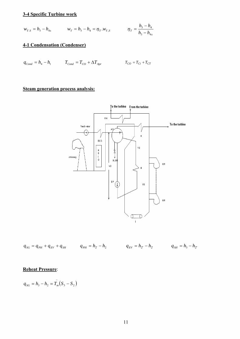
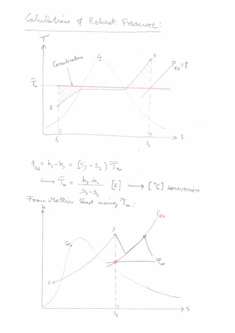
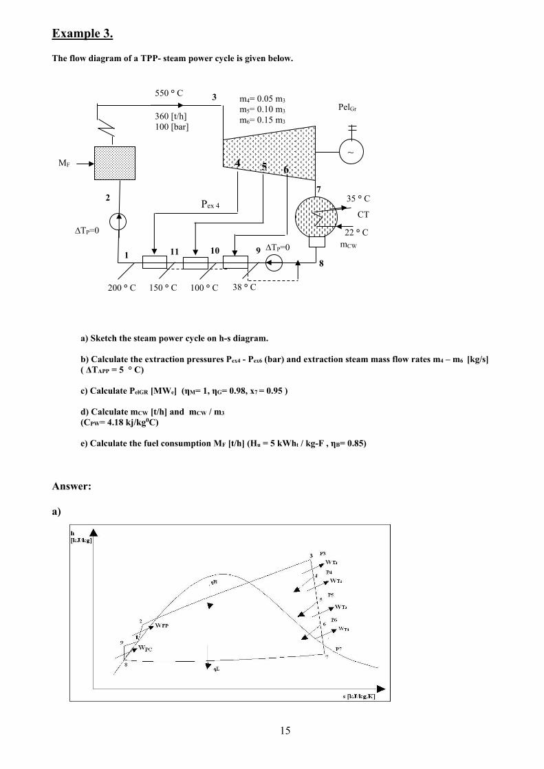
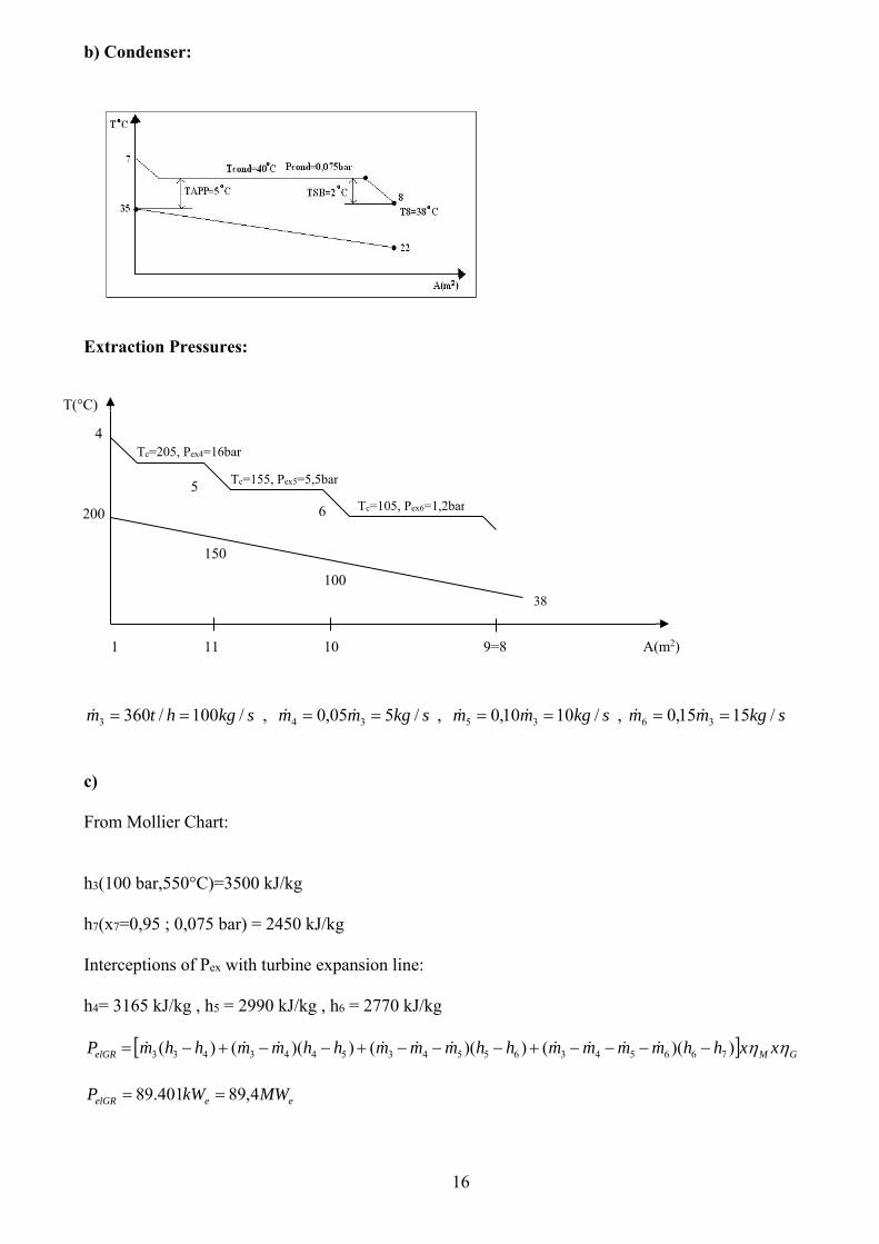
Example 3. The flow diagram of a TPP- steam power cycle is given below. Answer: a)

a) Sketch the steam power cycle on h-s diagram. b) Calculate the extraction pressures Pex4 - Pex6 (bar) and extraction steam mass flow rates m4 – m6 [kg/s] ( ΔTAPP = 5 ° C) c) Calculate PelGR [MWe] (ηM= 1, ηG= 0.98, x7 = 0.95 ) d) Calculate mCW [t/h] and mCW / m3

(CPW= 4.18 kj/kg0C) e) Calculate the fuel consumption MF [t/h] (Hu = 5 kWht / kg-F , ηB= 0.85)

~

∆TP=0

MF

3

4

2 Pex 4 35 ° C

22 ° C mCW

PelGr

5 6

550 ° C 360 [t/h] 100 [bar]

1

200 ° C 150 ° C 100 ° C

7

8

CT

9 10 11

m4= 0.05 m3 m5= 0.10 m3 m6= 0.15 m3

38 ° C

∆TP=0

16

b) Condenser:

Extraction Pressures:

skghtm /100/3603 ==& , skgmm /505,0 34 == && , skgmm /1010,0 35 == && , skgmm /1515,0 36 == && c) From Mollier Chart: h3(100 bar,550°C)=3500 kJ/kg h7(x7=0,95 ; 0,075 bar) = 2450 kJ/kg Interceptions of Pex with turbine expansion line: h4= 3165 kJ/kg , h5 = 2990 kJ/kg , h6 = 2770 kJ/kg

[ ] GMelGR xxhhmmmmhhmmmhhmmhhmP ηη))(())(())(()( 766543655435443433 −−−−+−−−+−−+−= &&&&&&&&&&

eeelGR MWkWP 4,89401.89 ==

38100

150

200

Tc=205, Pex4=16bar

6

5

4

Tc=155, Pex5=5,5bar

Tc=105, Pex6=1,2bar

11 10 9=81

T(°C)

A(m2)

17

d)

)35()22( 8777 xcmhmxcmhm pwcwpwcw &&&& +=+

skgxc

xchmmmmc

hhmmpw

pw

pwcw /2951

)2235(18,4)3818,42450)(15105100(

)2235()38)((

)2235()( 76543877 =

−−−−−

=−

−−−−=

−−

=&&&&&

&

51,293

=mmcw

&

&

e) hthkgxFkgkWh

kgkJxskgxH

hhmxH

QMtBuBu

JGF /7,62/62682

85,0)/(5)/)(20018,43500)(/(100)( 233 ==

−−

=−

==ηη

&

Example 4. For a coal fired TPP the following data are given:

t1≈t2=165 oC, t3=550 oC, P3=40 bar, m1=m2=m3=360 t/h, x4=0,95, tcwi=20 oC, tcwo=29 oC, t6=40 oC, t7=115 oC, All Heat Exchangers: ΔTAPR=5 oC, ΔTSC=2 oC, Cpw=4.18 [kJ/kgoC]

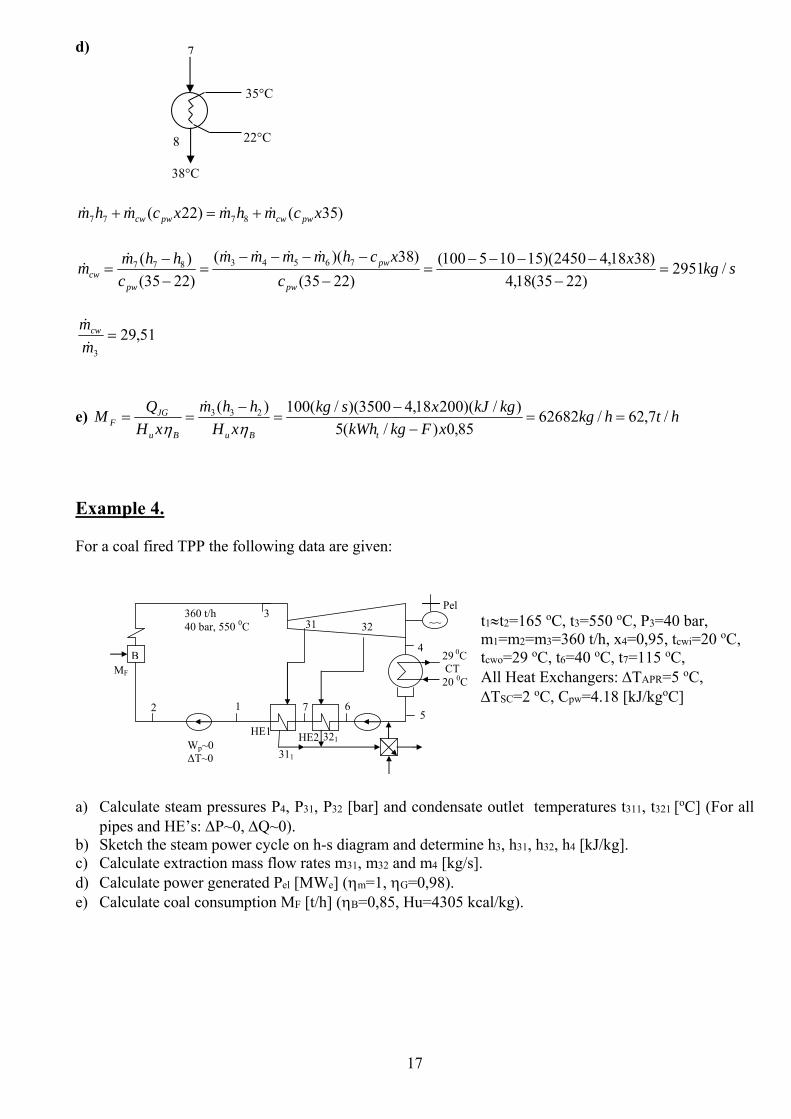
a) Calculate steam pressures P4, P31, P32 [bar] and condensate outlet temperatures t311, t321 [oC] (For all

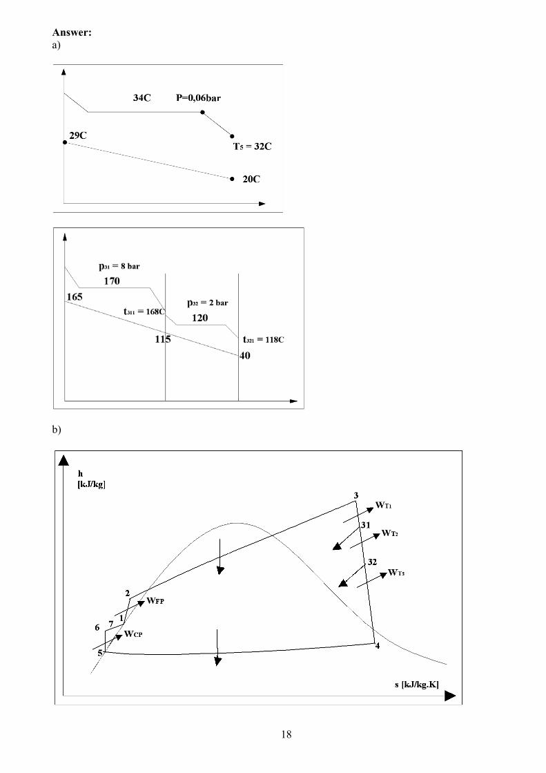
pipes and HE’s: ΔP~0, ΔQ~0). b) Sketch the steam power cycle on h-s diagram and determine h3, h31, h32, h4 [kJ/kg]. c) Calculate extraction mass flow rates m31, m32 and m4 [kg/s]. d) Calculate power generated Pel [MWe] (ηm=1, ηG=0,98). e) Calculate coal consumption MF [t/h] (ηB=0,85, Hu=4305 kcal/kg).

7

38°C

35°C

22°C 8

360 t/h 3 40 bar, 550 0C

Wp~0 ΔT~0

B

1

2

7

6

4

5 HE1

29 0C CT 20 0C

~~ 31 32

MF

Pel

HE2 311

321

18

Answer: a)

b)

19

kgkjhkgkjhkgkjh

kgkjbarCh

/2565/2925/3195

/3560)40,550(

4

32

31

03

===

=

c)

skgmmmm

skgm

skgskgm

hhmhhmskghtmmmmm

/73.78

/89.1211818.42925

)40115(18.4100

/38.816818.43195

)115165(18.4/100

)()(/100/360

323134

32

31

343131177

67321

=−−=

=×−−×

=

=×−−×

=

−=−======

&&&&

&

&

&&

Pel= [ m& 3(h3-h31) + ( m& 3- m& 31)(h31-h32) + ( m& 3- m& 31- m& 32)(h32-h4)] . ηM.ηG

=100(3560-3195) + ( 100-8.38) (3195-2925) + (100-8.38-12.89) (2925-2565) Pel=89.6 MWel d)

[ ]htM

skgkcalkjkgkcal

kgkjskgM

hhmHM

F

F

BuF

/6.67

/77.1885.0/18.4/4305

/)16518.43560(/100)( 233

=

=××

×−=

−=

&

&

&& η

20

Brayton Power Cycle (GT-TPP):

( ) GMCTGelGT wwmP ηη ..Σ−Σ=− & CC

CTBPC q

ww −=η GMCCBPCGTnet

ηηηηη ...=

1-2s (Isentropic Compression work) ⎥⎦

⎤⎢⎣

⎡kgkJ

⎥⎥⎥

⎦

⎤

⎢⎢⎢

⎣

⎡−⎟⎟

⎠

⎞⎜⎜⎝

⎛=−=

−

1..

1

1

21112,

kk

psSC PPTchhw ( )12, 21 ttCw SPSC S −= −

−

1-2( Poly. Comp. Work)

( )12,

12 21 ttCw

hhw P

C

SCC −==−= −

−

η ⎥

⎦

⎤⎢⎣

⎡⎥⎦⎤

⎢⎣⎡=

kgkJw

skgmP CGCom .& [kW]

2-3 (Heat Gen.)

23 hhqCC −= ⎥⎦

⎤⎢⎣

⎡kgkJ ( )2323 ttCq pCC −=

−

3-4s (Isent. Exp. Process)

( )sPsST ttChhw s 4343, 43 −=−= −

−

⎥⎥⎥

⎦

⎤

⎢⎢⎢

⎣

⎡

⎥⎦

⎤⎢⎣

⎡−=

−k

k

PST PPTcw

1

3

433, 1.. [kJ/kg]

3-4(Poly.Exp.Work)

( ) STTPT wttChhw ,4343 .43 η=−=−= −

−

[kJ/kg]

21

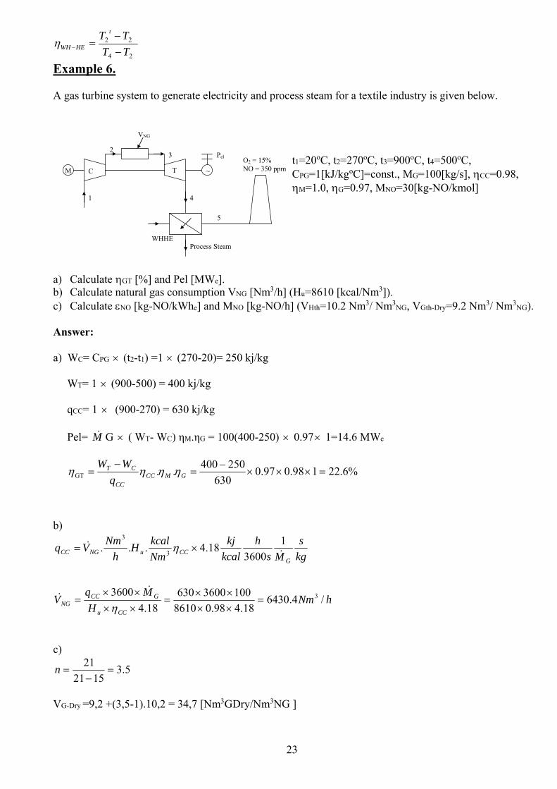
Example 5. The flow diagram of a simple GT-Power plant is given below. 3

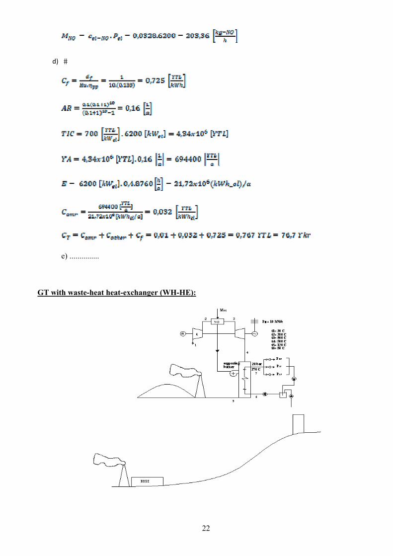
a) Skech the GT-Power cycle on h – s diagram b) Calculate Pel [MWe] c) Calculate emission factor ε el [kg-NO / kWhel] and M NO [kg –NO / h]

(VGth = 10 Nm3 / kg, VHth = 9.5 Nm3 / kg, Hu = 10 kWh /kg, MN= 14 kg/kmol, MO = 16 kg/kmol) d) Calculate CT [TL / kWhel]) (Coth = 1 [Ykr / kWhel], gF =1 [YTL/kg], F = 10 [%] , n Amr = 10 years, SIC= 700 [YTL / kWe, FL = 0.4 ) e) Selling price of electricity for the time being is approximately 10 Ykr / kWhel . Discuss the results. What can you do to this plant so that it can be operated economically?

Answer:

a) h-s diagram

b)

c)

2

C T

1 4

CC

Pel

NO=1000 [ppm] O2 = 15 [%]

t1 = 30 oC, t2= 300 oC t3 = 850 oC t4 = 500 oC, ηm = 1 , ηG = 0,97, ηCC = 0,98 CPG = 1 [ kj / kg 0C] = cont., mG = 80 [kg/s]

22

d) �

e) ...............

GT with waste-heat heat-exchanger (WH-HE):

23

24

22

TTTT ı

HEWH −−

=−η

Example 6. A gas turbine system to generate electricity and process steam for a textile industry is given below.

t1=20oC, t2=270oC, t3=900oC, t4=500oC, CPG=1[kJ/kgoC]=const., MG=100[kg/s], ηCC=0.98, ηM=1.0, ηG=0.97, MNO=30[kg-NO/kmol]

a) Calculate ηGT [%] and Pel [MWe]. b) Calculate natural gas consumption VNG [Nm3/h] (Hu=8610 [kcal/Nm3]). c) Calculate εNO [kg-NO/kWhe] and MNO [kg-NO/h] (VHth=10.2 Nm3/ Nm3NG, VGth-Dry=9.2 Nm3/ Nm3NG). Answer: a) WC= CPG × (t2-t1) =1 × (270-20)= 250 kj/kg WT= 1 × (900-500) = 400 kj/kg qCC= 1 × (900-270) = 630 kj/kg Pel= M& G × ( WT- WC) ηM.ηG = 100(400-250) × 0.97× 1=14.6 MWe

%6.22198.097.0630

250400..GT =×××−

=−

= GMCCCC

CT

qWW

ηηηη

b)

hNmH

MqV

kgs

Msh

kcalkj

NmkcalH

hNmVq

CCu

GCCNG

GCCuNGCC

/4.643018.498.08610

100360063018.4

3600

13600

18.4...

3

3

3

=××××

=××××

=

×=

η

η

&&

&&

c)

5.31521

21=

−=n

VG-Dry =9,2 +(3,5-1).10,2 = 34,7 [Nm3GDry/Nm3NG ]

O2 = 15% NO = 350 ppm M C

1

2

T

Pel

~

WHHE Process Steam

3

4

VNG

5

24

.

GT with Reheat

M

CT

WW

η=

1 ( ) GMTGGT wmP ηη ..

2&= GM

cc

cc

cc

cc

TGT qq

wηη

ηη

η ..

2

2

1

1

2

+=

Co-Generation PP:

LHVmQP

F

IndelCPP .&

&+=η

Combined Cycle PP

25

LHVmPP

F

STelGTelCCPP .&

−− +=η

Waste Heat Recovery Texhaust min. > Tdew

26

27

28

Critical insulation thickness?