Composite Focus Measure for High Quality Depth Maps Parikshit Sakurikar and P. J. Narayanan Center for Visual Information Technology - Kohli Center on Intelligent Systems, International Institute of Information Technology - Hyderabad, India {parikshit.sakurikar@research.,pjn@}iiit.ac.in Abstract Depth from focus is a highly accessible method to esti- mate the 3D structure of everyday scenes. Today’s DSLR and mobile cameras facilitate the easy capture of multi- ple focused images of a scene. Focus measures (FMs) that estimate the amount of focus at each pixel form the basis of depth-from-focus methods. Several FMs have been pro- posed in the past and new ones will emerge in the future, each with their own strengths. We estimate a weighted com- bination of standard FMs that outperforms others on a wide range of scene types. The resulting composite focus mea- sure consists of FMs that are in consensus with one another but not in chorus. Our two-stage pipeline first estimates fine depth at each pixel using the composite focus measure. A cost-volume propagation step then assigns depths from con- fident pixels to others. We can generate high quality depth maps using just the top five FMs from our composite focus measure. This is a positive step towards depth estimation of everyday scenes with no special equipment. 1. Introduction Recovering the 3D structure of the scene from 2D images has been an important pursuit of Computer Vision. The size, relative position and shape of scene objects play an impor- tant role in understanding the world around us. The 2.5D depth map is a natural description of scene structure, cor- responding to an image from a specific viewpoint. Multi- camera arrangements, structured lights, focus stacks, shad- ing etc., can all recover depth maps under suitable condi- tions. Users’ experience and understanding of the envi- ronment around them can be improved significantly if the 3D structure is available. The emergence of Augmented and Virtual Reality (AR/VR) as an effective user interaction medium enhances the importance of easy and inexpensive structure recovery of everyday environments around us. Depth sensors using structured lights or time-of-flight cameras are common today, with a primary use as game appliances [13]. They can capture dynamic scenes but have Figure 1. A coarse focal stack of an outdoor scene and its surface- mapped 3D depth is shown from two different viewpoints. The depth-map is computed using our composite focus measure. The smooth depth variation along the midrib of the leaf is clearly visi- ble in the reconstructed depth rendering. serious environmental, resolution and depth-range limita- tions. Multi-camera setups are more general, but are un- wieldy and/or expensive. Focus and defocus can also pro- vide estimates of scene depth. Today’s DSLR cameras and most mobile cameras can capture focal stacks by manipulat- ing the focus distance programmatically. Thus, depth from focus is a promising way to recover 3D structure of static scenes as it is accessible widely. We present a scheme to recover high quality depth maps of static scenes from a focal stack, improving on previous depth-from-focus (DfF) methods. We show results on sev- eral everyday scenes with different depth ranges and scene complexity. Figure 1 is an example of robust depth recovery that we facilitate. The specific contributions of this paper are given below. 1. Composite Focus Measure: A focus measure (FM) to evaluate the degree of focus or sharpness at an image pixel is central to DfF. Several focus measures have been used for different scenarios. We combine them into a composite focus measure (cFM) by analyzing their consensus and correlation with one another over 150 typical focal stacks. The cFM is a weighted com- bination of individual adhoc FMs with weights com- 1614
Transcript
Composite Focus Measure for High Quality Depth Maps
Parikshit Sakurikar and P. J. Narayanan
Center for Visual Information Technology - Kohli Center on Intelligent Systems,
International Institute of Information Technology - Hyderabad, India
{parikshit.sakurikar@research.,pjn@}iiit.ac.in
Abstract
Depth from focus is a highly accessible method to esti-
mate the 3D structure of everyday scenes. Today’s DSLR
and mobile cameras facilitate the easy capture of multi-
ple focused images of a scene. Focus measures (FMs) that
estimate the amount of focus at each pixel form the basis
of depth-from-focus methods. Several FMs have been pro-
posed in the past and new ones will emerge in the future,
each with their own strengths. We estimate a weighted com-
bination of standard FMs that outperforms others on a wide
range of scene types. The resulting composite focus mea-
sure consists of FMs that are in consensus with one another
but not in chorus. Our two-stage pipeline first estimates fine
depth at each pixel using the composite focus measure. A
cost-volume propagation step then assigns depths from con-
fident pixels to others. We can generate high quality depth
maps using just the top five FMs from our composite focus
measure. This is a positive step towards depth estimation of
everyday scenes with no special equipment.
1. Introduction
Recovering the 3D structure of the scene from 2D images
has been an important pursuit of Computer Vision. The size,
relative position and shape of scene objects play an impor-
tant role in understanding the world around us. The 2.5D
depth map is a natural description of scene structure, cor-
responding to an image from a specific viewpoint. Multi-
camera arrangements, structured lights, focus stacks, shad-
ing etc., can all recover depth maps under suitable condi-
tions. Users’ experience and understanding of the envi-
ronment around them can be improved significantly if the
3D structure is available. The emergence of Augmented
and Virtual Reality (AR/VR) as an effective user interaction
medium enhances the importance of easy and inexpensive
structure recovery of everyday environments around us.
Depth sensors using structured lights or time-of-flight
cameras are common today, with a primary use as game
appliances [13]. They can capture dynamic scenes but have
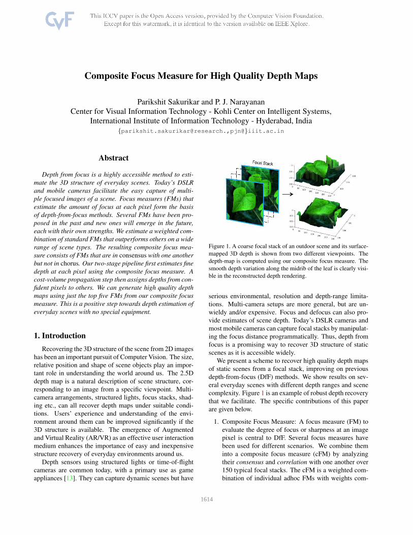
Figure 1. A coarse focal stack of an outdoor scene and its surface-
mapped 3D depth is shown from two different viewpoints. The
depth-map is computed using our composite focus measure. The
smooth depth variation along the midrib of the leaf is clearly visi-
ble in the reconstructed depth rendering.
serious environmental, resolution and depth-range limita-
tions. Multi-camera setups are more general, but are un-
wieldy and/or expensive. Focus and defocus can also pro-
vide estimates of scene depth. Today’s DSLR cameras and
most mobile cameras can capture focal stacks by manipulat-
ing the focus distance programmatically. Thus, depth from
focus is a promising way to recover 3D structure of static
scenes as it is accessible widely.
We present a scheme to recover high quality depth maps
of static scenes from a focal stack, improving on previous
depth-from-focus (DfF) methods. We show results on sev-
eral everyday scenes with different depth ranges and scene
complexity. Figure 1 is an example of robust depth recovery
that we facilitate. The specific contributions of this paper
are given below.
1. Composite Focus Measure: A focus measure (FM) to
evaluate the degree of focus or sharpness at an image
pixel is central to DfF. Several focus measures have
been used for different scenarios. We combine them
into a composite focus measure (cFM) by analyzing
their consensus and correlation with one another over
150 typical focal stacks. The cFM is a weighted com-
bination of individual adhoc FMs with weights com-
11614
puted off-line. In practice, a combination can involve
as few as two FMs or as many as all of them.
2. Depth Estimation and Propagation: We use a two-stage
pipeline for DfF, with the first stage estimating a fine
depth at each pixel using a Laplacian fit over the com-
posite focus measure. This gives both a depth estimate
and a confidence value for it. In the second stage, a
cost-volume propagation step distributes the confident
depth values to their neighborhoods using an all-in-
focus image as a guide.
We present qualitative and quantitative results on a large
number and variety of scenes, especially everyday scenes
of interest. The depth maps we compute can be used for
applications that RGBD images are used for, typically at
resolutions and fidelity higher than them.
2. Related Work
Depth from Focus/Defocus: The computation of depth
from multiple focused images has been explored in the
past [2, 4, 20, 29]. Defocus cues have also been used
[3, 7, 9, 19, 22, 23, 30] to estimate scene depth. In most
methods, depth is estimated from the peak focus slice com-
puted using per-pixel focus measures. Pertuz et al. [24] an-
alyze and compare several focus measures independently
for DfF. They conclude that Laplacian based operators are
best suited under normal imaging conditions. In [20], the
Laplacian focus measure is used to compare classical DfF
energy minimization with a variational model. A new RDF
focus measure was proposed in [28], with a filter shape de-
signed to encode the sharpness around a pixel using both
local and non-local terms. Mahmood et al. [18] combined
three well known focus measures (Tenengrad, Variance and
Laplacian Energy) in a genetic programming framework.
Boshtayeva et al. [4] described anisotropic smoothing over
a coarse depth map computed from focal stacks. Suwa-
janakorn et al. [29] proposed a joint optimization method
to solve the full set of unknowns in the focal stack imag-
ing model. Methods such as [4, 20] can benefit from the
composite focus measure we propose in this work.
Focal Stacks and All-in-focus Imaging: Focal stacks are
images of the scene captured with same camera settings
but varying focus distances. Usually a focal stack has each
scene point in clear focus in one and only one image. Fo-
cal stacks enable the generation of all-in-focus (AiF) im-
ages where each pixel corresponds to its sharpest version.
Generating the best in-focus image has been the goal for
several works [1, 15, 21, 32]. Reconstruction of novel fo-
cused images has also been achieved using focal stacks
[14, 10, 11, 21, 29, 33].
Focal stacks can be captured without special equipment
or expensive cameras. Several mobile devices can be pro-
grammed to capture multiple focused images sequentially.
Region-based focus stacking has also been used in the past
on mobile devices [26]. Most DSLRs can automatically