'Composite Materials'. In: Encyclopedia of Polymer Science ...nguyen.hong.hai.free.fr/EBOOKS/SCIENCE...

282 COMPOSITE MATERIALS Vol. 9

COMPOSITE MATERIALS

Introduction

Composite materials are made by combining two or more materials to give aunique combination of properties. Many common materials are indeed “com-posites,” including wood, concrete, and metals alloys. However, fiber-reinforcedcomposite materials differ from these common materials in that the constituentmaterials of the composite (eg the two or more phases) are macroscopically distin-guishable and eventually mechanically separable. In other words, the constituentmaterials work together but remain essentially in their original bulk form (apartfrom the thin hybrid interface between the phases).

The main component of a composite is the matrix material. The reinforce-ment (qv) can be fibers, particulates, or whiskers. The fibers can be continuous,long, or short. In advanced composites, the fibers (ie the reinforcing phase) arepresent as unidirectional strands or woven fabric and provide strength and stiff-ness to the composite. The matrix acts as a load transfer medium assuring rigidityand protects the fibers and the whole composite from environmental attack. Shortchopped fibers and mat are used in nonstructural polymer matrix composites.In these cases the fibers provide comparatively less strength and stiffness to thecomposite.

Fiber-reinforced polymer matrix composites are the most common advancedcomposites. Early glass-fiber-reinforced composites resins were used in the 1930sto build parts of boats and aircraft. Since the 1970s, application of composites haswidely increased owing to the development of new fibers such as carbon, boron,and aramids (see HIGH PERFORMANCE FIBERS). Thermosetting polymers such asepoxy, polyester, and urethane resins are, among the others, the most widely usedmatrices of advanced composites. (see THERMOSETS). In the 1980s the develop-ment of new, cost-effective thermoplastic polymers such as PEEK (poly-ether-ether-ketone) and PEI (Poly-ether-imides) allowed the development of a new classof high performance composites (see ENGINEERING THERMOPLASTICS, OVERVIEW;POLYIMIDES).

Thermosetting and thermoplastic matrix composites are in many ways su-perior materials compared to common metals and ceramic materials. Their re-liability is confirmed by their large use in the aerospace industry. Mechanicaladvantages of polymer composites are expressed in terms of two main parame-ters (ie specific modulus and strength) reflecting the key role of density on theselection of high performance materials. The specific modulus Es is defined as theratio between the Young’s modulus E and density ρ of the material. The other pa-rameter, the specific strength (σ s), is defined as the ratio of the ultimate strengthσ ult and the density

Es = Eρ

(1)

σs = σult

ρ(2)

Encyclopedia of Polymer Science and Technology. Copyright John Wiley & Sons, Inc. All rights reserved.

Vol. 9 COMPOSITE MATERIALS 283

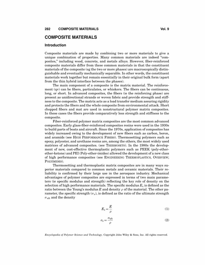
The coefficient of thermal expansion (CTE) of composite structures can bemade close to zero by selecting suitable materials and lay-up sequence. Dimen-sional stability is, in fact, one of the key requirements that many metals cannotsatisfy (owing to their higher CTE) in aerospace applications. A CTE that can betailored for a specific application gives rise to an increased amount of design flex-ibility with respect to common metals. In Table 1 the relevant thermomechanicalproperties of common and fiber-reinforced composite materials are reported. Thelast three columns of Table 1 explain why specific stiffness, strength, and CTE are,among the others, the key parameters in the selection of composite materials inaerospace applications where both performance and cost are a concern. High spe-cific performance of composite materials allows weight saving, with consequentincrease in payload and fuel savings. Composite materials can be highly fatigue-and corrosion-resistant, with enhanced life and reduced maintenance costs. Thefollowing drawbacks represent limits in using polymer-based composites:

(1) The high cost of fabrication of composites for aerospace applications is stilla critical issue. Today most of the effort and investment in this area is de-voted toward improving processing and manufacturing techniques in orderto lower costs. Medium performance composites, on the contrary, can bemade using manufacturing techniques such as sheet molding compound(SMC), structural reinforced injection molding (SRIM), and resin transfermolding (RTM), in which both the cost and the production time have beenconsistently optimized to compete within the automotive industry.

(2) Unlike metals, fiber-reinforced composites are anisotropic, that is, theirproperties depend on both the fiber orientation and the lay-up sequencein the laminate. In-plane quasi-isotropic materials can, however, be madeby opportune selection of a lay-up sequence (eg a [0/±45/90]2s laminationsequence realizes in-plane equivalent properties from an engineering pointof view) or when continuous random mats of fibers are utilized as the rein-forcing system (this is the case in parts obtained by SRIM or RTM). In bothcases, however, the fibers remain perpendicular to the third direction, andit is this drawback that renders the design procedures far more complicatedand intensive than those normally utilized for isotropic materials. In otherwords, while monolithic materials such as aluminum require only two elas-tic constants to establish the stress–strain relationship in each body pointfor a given system of forces acting on it, composite materials require manymore elastic constants. For example, in unidirectional composites (whereall the fibers lay in one direction) under plane stress conditions (no out-of-plane loads) four elastic constants are required. In addition, the mechanicalcharacterization of a composite structure is far more complex than that of ametal structure if one considers that the techniques for the evaluation andmeasurement of some composite properties, such as fracture toughness andcompressive strength, are still debatable.

(3) The reinforcing fibers in composites offer unique properties but create com-plications in recycling. Thermoplastic composites have the potential of pri-mary and secondary recycling since the reprocessing of waste can resultin a product with the same or comparable properties, whereas thermoset

Table 1. Specific Modulus, Strength, and CTE of Typical Fibers and Bulk Materials.

Young’s Specific Ultimate SpecificDensity, modulus, modulus, strength, strength,

Material mg/m3 GPa (GPa · m3)mg GPa (GPa · m3)/mg CTE, 10− 6/◦C− 1

Steel 7.85 200 25.5 0.38–1.79 0.048–0.23 30–51Aluminum 2.7 70 25.9 0.09–0.572 0.033–0.21 64–71Titanium 4.5 110 24.4 0.24–1.17 0.053–0.26 25–38Aramid 1.44 131 91 3.6–4.1 2.5–2.85 Id:−6.0, td:180a

Graphite 1.78–2.15 228–724 106–407 1.5–4.8 0.70–2.70 Id:−1.8, td:30Glass 2.58 72.5 28.1 3.45 1.34 15Alumina 3.95 379 96 1.38 0.35 22Unidirectional AS4 graphite–epoxy (V f = 70%) 1.64 161 98.2 2.77 1.68 Id:−3.84 × 10− 2, td:26Unidirectional E-glass–epoxy (V f = 50%) 1.93 38.34 19.86 0.93 0.48 Id: 7.37, td: 28.62Cross-ply AS4 graphite–epoxy (V f = 58%) 1.57 77.45 48.98 – – 1.56Cross-ply E-glass–epoxy (V f = 40%) 1.8 21.05 11.69 – 6aId = longitudinal direction, td = transverse direction.

284


composite scraps usually are tertiary recycled (in order to recover the fibersso they can be reused in molding compounds) or essentially burned off.

(4) Repairing composite parts is a very complex process and not alwaysaccessible.

(5) Most of the effectiveness of nondestructive techniques for the inspectionof metal parts (such as eddy currents, X-ray) is lost when it comes todetection of flaws and cracks in composite structures, unless appropriatemodifications are made to the instrumentation hardware or the inspec-tion procedure. Ultrasound, laser (shearography), and acoustic emissiontechniques are usually preferred for inspecting the crack initialization (seeNONDESTRUCTIVE TESTING).

Many of the above drawbacks forced the composite industry to focus signif-icant effort on the development of manufacturing procedures in which the fabri-cation process is controlled with the highest level of real-time monitoring tools. Itis well established that the quality of a composite structure depends almost com-pletely on the process quality. Controlling the manufacturing process depends,first of all, on a deep knowledge of the overall physical and chemical changesoccurring within the part. Mathematical modeling then provides estimates of op-timum process parameters for a given manufacturing process to produce a highquality product.

Composite Manufacturing Techniques

Composite parts are made using either thermoset or thermoplastic resins withsome form of reinforcements. Techniques for manufacturing polymer matrix com-posites are covered in Composites, Fabrication (qv). Filament winding and roboticwinding are used for making pipes and tanks. Pultrusion is used for low cost highvolume productions. Autoclave processing is used when high quality panels andstructures sometimes having complex shapes are required. RTM is used exten-sively to make small and large complex structural parts in a cost-effective mannerusing low cost tooling. Compression molding processes are widely used in the au-tomotive industry for high volume production capabilities and injection molding(qv) is adopted when the production rate is a critical issue, mainly for consumerand automotive applications.

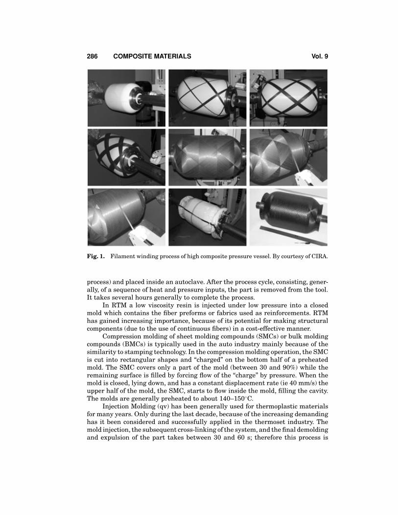
Filament winding consists of drawing resin-impregnated fibers that arewound over a mandrel. Winding patterns are decided at the design stage depend-ing on the desired properties of the product. The winding process of a high qualitypressure vessel is shown in Fig. 1.

Pultrusion is a simple, continuous process in which resin-impregnated fibersare pulled through a die to make a part. During passage through the heated dieresin-impregnated yarns consolidate due to the incoming cross-linking reaction.Objects with constant cross-section and smooth finish can be obtained.

Autoclave processing is used with prepregs with lay-up realized by auto-mated means or by hand. The assembly is vacuum-bagged in order to minimizethe presence of volatile substances (responsible for void/defect growth during the


Fig. 1. Filament winding process of high composite pressure vessel. By courtesy of CIRA.

process) and placed inside an autoclave. After the process cycle, consisting, gener-ally, of a sequence of heat and pressure inputs, the part is removed from the tool.It takes several hours generally to complete the process.

In RTM a low viscosity resin is injected under low pressure into a closedmold which contains the fiber preforms or fabrics used as reinforcements. RTMhas gained increasing importance, because of its potential for making structuralcomponents (due to the use of continuous fibers) in a cost-effective manner.

Compression molding of sheet molding compounds (SMCs) or bulk moldingcompounds (BMCs) is typically used in the auto industry mainly because of thesimilarity to stamping technology. In the compression molding operation, the SMCis cut into rectangular shapes and “charged” on the bottom half of a preheatedmold. The SMC covers only a part of the mold (between 30 and 90%) while theremaining surface is filled by forcing flow of the “charge” by pressure. When themold is closed, lying down, and has a constant displacement rate (ie 40 mm/s) theupper half of the mold, the SMC, starts to flow inside the mold, filling the cavity.The molds are generally preheated to about 140–150◦C.

Injection Molding (qv) has been generally used for thermoplastic materialsfor many years. Only during the last decade, because of the increasing demandinghas it been considered and successfully applied in the thermoset industry. Themold injection, the subsequent cross-linking of the system, and the final demoldingand expulsion of the part takes between 30 and 60 s; therefore this process is


particularly considered when very high volume production is requested. In somecases, using multiple-cavity molds for the consolidation of different element partsat the same time can further increase the production rate.

Many other techniques have been developed over the years. However, eachmanufacturing process consists of four basic steps, wetting/impregnation, lay-up,consolidation, and solidification, which in case of composites require low energycompared with those for traditional materials. In fact, composites do not havehigh pressure and temperature requirements for part processing as comparedwith metal. This is the reason why composite processing techniques such as thosedescribed above have the potential of producing complex, high strength, high stiff-ness, and near-net-shape structures. Therefore the applications of polymer matrixcomposites range from the aerospace industry to the sporting goods. Compositesare the material of choice in space applications owing essentially to two factors:high specific modulus and strength, and dimensional stability. Graphite–epoxycomposites are increasingly used in bicycles, sometimes allowing frames to con-sist of one lightweight piece, or in golf club shafts, using the saved weight inthe head. Tennis and racquetball rackets with graphite–epoxy frames are nowcommonplace. The military aircraft industry has mainly led the use of polymercomposites in structural applications while in commercial airlines the use of com-posites has been conservative because of safety concerns. The graphite–epoxy andaramid honeycomb tail fin of Airbus A310-300 is an example of using compositesin the primary structure in commercial airlines. The weight of the tail fin wasreduced by 300 kg, together with the number of parts, which decreased from 2000to 100. Infrastructure applications of polymer composites include bridges—due tolow weight, corrosion resistance, longer life cycles, and limited earthquake dam-age. The application of fiber glass in boats is well known even when hybrids ofKevlar–glass/epoxy are now receiving attention because of the improved weightsavings, vibration damping, and impact resistance.

Today’s automobile industry uses low amounts of composite parts owing tothe unavailability of cost-effective manufacturing techniques. Nowadays about 8%of automobile parts are made of composites.

Process Modeling

During the fabrication process (eg RTM, autoclave, filament winding) a combina-tion of pressure–temperature steps are applied with given histories in order toassure well-consolidated parts with minimum defects. The solidification or cur-ing process involves a number of physical, chemical, and mechanical phenomenain the composite materials. Generally speaking, the formation of a structure dueto cross-linking reactions or to the melting and consolidation of thermoplasticpolymers is the macroscopic effect of heat and pressure inputs: in real terms con-tinuous changes in degree of cure or crystallinity, gelation (the formation of aninfinite polymer network as a consequence of chemical reaction) and vitrification(the passage from a molten/rubbery to a glassy state) occur. As a consequenceof the above phenomena, the evolving chemical and thermal shrinkage give riseto the development of stress and strain within the part, whereas the presence


of volatiles in the form of residual plasticizing agents or unreacted resins caneventually induce void growth and resin–fiber debonding.

In all, thermal shrinkage, chemical shrinkage, time–temperature–degree ofcure dependent resin properties, viscosity, and structural relaxation shrinkageare the matrix properties to control. Therefore, since the evolution of polymerproperties is strongly influenced by processing history, each parameter has tobe investigated at each stage of the manufacturing process. Moreover consideringthat the level of temperature reached during the manufacturing of composite partsdoes not affect the fiber content, investigations are almost always carried out onthe polymer system matrix. Significant progress has been made in quantitativelyevaluating process-related parameters such as mold shape, mold material andsurface, void content, fiber volume fraction, lay-up sequence. However, consider-able work remains to be done to account for constituent resin-related properties.In particular, when new resins are developed a number of experimental tests arenecessary to completely characterize the resin (such as toughened epoxies) so asto perform a general analysis of the physical and chemical phenomena and to codeit by mathematical tools.

Mathematical modeling of a manufacturing process provides a tool forthe process control with minimum costs and high quality production. Typicalaerospace manufacturing processes for composites are characterized by a two-step cure cycle. In such a cycle the temperature of the material is increased fromroom temperature to the first dwell temperature and this temperature is heldconstant for the first dwell period (∼1 h); during this stage the material reachesthe minimum value of viscosity to fill the mould and/or compact the whole system.The temperature is then increased again to the second dwell temperature and heldconstant for the second dwell period (∼2–8 h). Post-cure reaction takes place dur-ing this second stage. Following this second dwell period the part is cooled downto room temperature at a constant rate or by air to allow the extraction from themould. It is during the polymerization reaction that the strength and related me-chanical properties of the composite are developed, together with incipient flaws(eg voids, resin–fiber debonding) and residual stresses.

The transient heat transfer phenomena induce peculiar property changesat each body point. In this respect, the temperature profiles and the chemo-rheological functions (viscosity, degree of cure/crystallinity) need to be includedwithin the energy balance equation:

ρCP∂T∂t

= ∇(K∇T) + ρQ (3)

where ρ is the density, Cp is the specific heat, t is the time, K is the thermal conduc-tivity, and Q is the rate of heat generated either by the exothermic polymerizationreaction in the case of a thermosetting matrix system or by the crystallizationprocess for thermoplastic matrix.

From the micro-mechanical point of view, the process modeling strategiesmust consider simultaneous interplay of the following “intrinsic” factors: initialand boundary conditions in terms of pressure and temperature, fiber content andstacking, sequence of layers (ie ply-to-ply orientation), thermal shrinkage, chemi-cal shrinkage, time–temperature–degree of cure dependent resin properties, and


structural relaxation shrinkage. The above factors can play a different role whenan even more complex scenario arises for thick composite parts. Therefore a de-tailed analysis of temperature distribution during the process is crucial for thedetermination of the complex evolution of the properties at each material pointof the composite part. A simple analogy could be made with metals in order tounderstand this complex scenario. The evolution of the structure for metals in-evitably leads to a distribution of grain size as a result of the different temperatureprofiles experienced during the forming process. In the case of polymeric matri-ces, the same assumption can be reasonably made considering that each materialpoint will undergo a completely different temperature profile, owing to the relativeposition occupied in respect to the heat source. For this reason, a thermosettingsystem matrix necessarily presents a distribution of polymerization reactions ateach body point, according to the experienced thermal histories; in the case of ther-moplastic systems, because of the strong dependency of the crystallization processupon the temperature profile, a distribution of grain size through the thickness (ieskin–core fine to coarse structure) is obtained. The temperature distribution canbe suitably determined using finite element analysis (FEA) software; the tem-perature at a given point in the structure depends on the boundary and initialconditions, as well as the materials’ properties evolution. In fact, as the evolu-tion of the structure is highly dependent on the thermal history, within a thickcomposite different material properties arise at each material point.

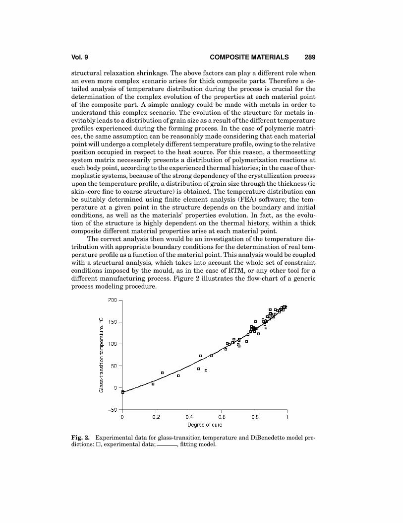
The correct analysis then would be an investigation of the temperature dis-tribution with appropriate boundary conditions for the determination of real tem-perature profile as a function of the material point. This analysis would be coupledwith a structural analysis, which takes into account the whole set of constraintconditions imposed by the mould, as in the case of RTM, or any other tool for adifferent manufacturing process. Figure 2 illustrates the flow-chart of a genericprocess modeling procedure.

Fig. 2. Experimental data for glass-transition temperature and DiBenedetto model pre-dictions: �, experimental data; , fitting model.


Different material parameters need to be quantified to be able to perform thethermostructural analysis. The complex interactions of the different phenomenaoccurring during the manufacturing process could be schematized as follows.

(1) Both crystallization and polymerization reactions are temperature-activated phenomena, allowing the transformation of the system from aliquid-like to an almost solid-like material. The structure evolution can besuitably monitored by a degree of conversion parameter, which follows ananalytical kinetics model.

(2) Thermal (specific heat, thermal conductivity) and viscoelastic properties ofthe material change during the process owing to both temperature varia-tions (as for traditional materials) and level of conversion.

(3) Variation of the specific volume can be originated by three different phe-nomena:

a. thermal expansion (or contraction) due to positive (negative) tempera-ture change,

b. chemical/physical shrinkage due to the densification (polymeriza-tion/crystallization) of the material according to the conversion level,and/or

c. contraction due to the thermodynamic instability associated with thenonequilibrium kinetics of glass transition (structural relaxation).

The experimental evaluation and the modeling of each contribution still rep-resent a difficult task for many researchers, and at the same time it is the mainissue for the correct prediction of

(1) the residual stress formation and warpage effect in thick composite parts(2) voids and flaw formation, and(3) resin flow behavior dependent compaction and consolidation feature.

Coupled with the energy equation along with the specific initial and bound-ary conditions, the mathematical description of the above factors (through theuse of suitable submodels for a given manufacturing process) allows the completeanalysis of a generic manufacturing process, providing at the same time a funda-mental “tool” for the production of high quality parts.

Cure Kinetics and Glass-Transition Model

As stated above, during the cure, at each level of conversion, a thermosettingmaterial could be assimilated to a completely new material with specific thermo-mechanical properties. Then, the possibility of following with a monitoring vari-able the level of conversion reached by the system during the manufacturing pro-cess represents an important issue.

Thermal analysis provides useful information upon which to constructan adequate kinetics model under both isothermal and dynamic temperature


conditions. The mathematical model selected on the basis of the experimentaldata generally represents the primary component in studies on the optimizationof thermoset molding processes (resin transfer molding, reaction injection mold-ing, prepreg cure, etc). Reliable methods are required to predict the degree ofconversion and to control the evolution of the exothermic heat of reaction. Correctkinetics models are also essential to predict the evolution of the structure undermore complicated temperature profiles; or to correlate the changes in thermal andmechanical properties of the neat resin through all the manufacturing processes.Thus, the knowledge of the level of conversion of the polymer matrix is fundamen-tal information to monitor the evolution of properties. Curing raw data neededto implement the kinetics models can be obtained, by nearly standardized proce-dures, through isothermal and dynamic differential scanning calorimetry (DSC)tests.

There are essentially two kinetic models used to describe thermoset-curingreactions.

(1) Phenomenological Models (macroscopic level) assume that there is an over-all order of reaction and fit this model to the experimental kinetic data.This type of model provides no information about the kinetic mechanismof the reaction and is predominantly used to provide models for industrialapplications.

(2) Mechanistic models (microscopic level) are derived from a rather complexanalysis of the individual reactions occurring during the cure, and requiredetailed measurements of the concentrations of reactants, intermediates,and products. Mechanistic models are much more complex than empiricalmodels, but are not restricted by changes in the composition of the system.

Despite the efforts that have been made in recent years, in the exploitationof kinetic models for polymerization of thermosetting resin systems (see Table 1),two main problems still arise:

(1) no general model for the cure mechanisms of all systems is available (al-though many authors in the past have already searched for a generalizedmodel), and

(2) in many cases, for a given resin system, different models are needed todescribe isothermal and nonisothermal experimental condition.

The first problem still represents a severe limitation on the industrial appli-cation of any monitoring or control system that requires significant prior knowl-edge of the cure kinetics, which will affect either the time or cost of production.Acquired thermal data are generally fitted with chose kinetics equation to estab-lish the best set of kinetics parameters to predict the conversion evolution for ageneric temperature history at every location.

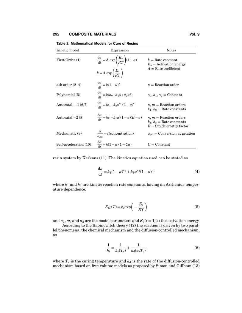
In Table 2, the most used kinetic equations are reported. Advances in thedescription of cure kinetics were recently used to model the cure of an RTM epoxy


Table 2. Mathematical Models for Cure of Resins

Kinetic model Expression Notes

First Order (1)dα

dt= A exp

(Ea

RT

)(1 − α)

k = A exp

(Ea

RT

)k = Rate constantEa = Activation energyA = Rate coefficient

nth order (2–4)dα

dt= k(1 − α)n n = Reaction order

Polynomial (5)dα

dt= k(a0+a1α+a2α

2) a0, a1, a2 = Constant

Autocatal. −1 (6,7)dα

dt= (k1+k2α

m)(1 − α)n n, m = Reaction ordersk1, k2 = Rate constants

Autocatal −2 (8)dα

dt= (k1+k2α)(1 − α)(B − α) n, m = Reaction orders

k1, k2 = Rate constantsB = Stoichiometry factor

Mechanistic (9)α

αgel= f (concentration) αgel = Conversion at gelation

Self-acceleration (10)dα

dt= k(1 − α)(1 − Cα) C = Constant

resin system by Karkans (11). The kinetics equation used can be stated as

dα

dt= k1(1 − α)n1 + k1α

n2 (1 − α)n1 (4)

where k1 and k2 are kinetic reaction rate constants, having an Arrhenius temper-ature dependence.

KiT(T) = kiexp(

− Ei

RT

)(5)

and n1, m, and n2 are the model parameters and Ei (i = 1, 2) the activation energy.According to the Rabinowitch theory (12) the reaction is driven by two paral-

lel phenomena, the chemical mechanism and the diffusion-controlled mechanism,as

1ki

= 1kc(Tc)

+ 1kd(α,Tc)

(6)

where Tc is the curing temperature and kd is the rate of the diffusion-controlledmechanism based on free volume models as proposed by Simon and Gillham (13)


in the following from:

kd(T) = kd0 exp(

− bf

)(7)

In the above equation b is an adjustable parameter to achieve a suitable fit,while the parameter f encapsulates the driving force of the diffusion-controlledmechanism by means of the Doolittle (14) equation, to model the free volume asfollows:

f (α) = (4.8×10− 4) [Tc − Tg(α)] + 2.5 × 10− 3 (8)

The diffusion-controlled mechanism occurs during vitrification in the latterstage of the reaction. It is obvious that for a chemical reaction to occur, reactivegroups are required to be close to each other and also to be orientated so thateventually the cross-link can be formed. In the early stages of the cure, when thematerial is very much in a liquid state, the rate of cure is predominantly con-trolled by chemical kinetics; this essentially means that in the “reaction zone” thetemperature of the system is capable of activating a reaction between monomers.Since these processes are very fast owing to the short characteristic times of theliquid state compared to the time of experimental observations, the rate coeffi-cient for the reaction is constant at constant temperature, hence the validity ofArrhenius-type analysis. Theoretical models of this stage of the cure have beenextensively discussed by Mita and Horrie (15) using a reptation theory model, andby Rozenberg (16), who also tried to determine the topological area of the reactionassociated with reactive groups that are isolated within the gelled structure. Ex-periments have demonstrated that analytical methods are not sensitive enoughto detect these unreacted groups and for this reason it is not possible to evaluatetheir concentration during the final stages of the curing process. It is clear then,that the overall reaction rate cannot be a function of the temperature alone, butthat a dependency on a structural parameter has to be included, which at certainisothermal temperatures will lower the reaction rate, limiting the extent of thereaction.

The glass-transition temperature can be regarded as a suitable structuralparameter for following the progressive evolution of the cross-linked system incase of diffusion-controlled mechanism; therefore, a suitable model is needed. Theevolution of the glass-transition temperature is modeled according to a widelyaccepted DiBenedetto equation (17), stated as follows:

Tg(α) = (1 − α)Tg0 + λαTg∞(1 − α) + λα

(9)

where Tg0 and Tg∞ are the glass-transition temperatures for the uncured andfully cured resin, respectively; λ is the adjustable parameter for a given resin sys-tem. Figure 3 reports the experimental determinate values of the glass-transitiontemperature along with the found model predictions.

Most of the time, the complete kinetics model can result in a multiparame-ter model characterized by nonunique set of best parameters. Therefore, reliable


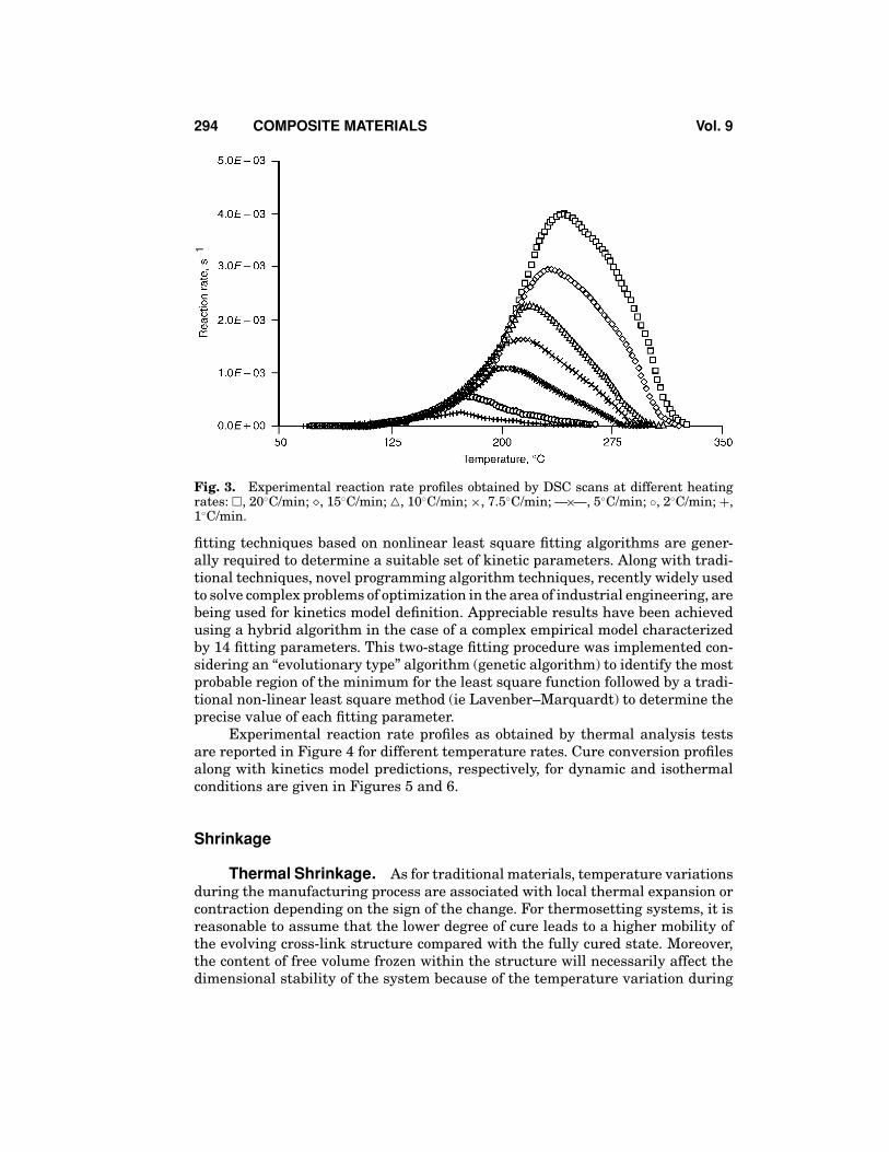
Fig. 3. Experimental reaction rate profiles obtained by DSC scans at different heatingrates: �, 20◦C/min; �, 15◦C/min; �, 10◦C/min; ×, 7.5◦C/min; —×—, 5◦C/min; ◦, 2◦C/min; +,1◦C/min.

fitting techniques based on nonlinear least square fitting algorithms are gener-ally required to determine a suitable set of kinetic parameters. Along with tradi-tional techniques, novel programming algorithm techniques, recently widely usedto solve complex problems of optimization in the area of industrial engineering, arebeing used for kinetics model definition. Appreciable results have been achievedusing a hybrid algorithm in the case of a complex empirical model characterizedby 14 fitting parameters. This two-stage fitting procedure was implemented con-sidering an “evolutionary type” algorithm (genetic algorithm) to identify the mostprobable region of the minimum for the least square function followed by a tradi-tional non-linear least square method (ie Lavenber–Marquardt) to determine theprecise value of each fitting parameter.

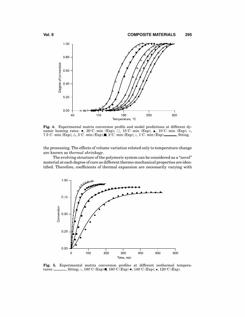
Experimental reaction rate profiles as obtained by thermal analysis testsare reported in Figure 4 for different temperature rates. Cure conversion profilesalong with kinetics model predictions, respectively, for dynamic and isothermalconditions are given in Figures 5 and 6.

Shrinkage

Thermal Shrinkage. As for traditional materials, temperature variationsduring the manufacturing process are associated with local thermal expansion orcontraction depending on the sign of the change. For thermosetting systems, it isreasonable to assume that the lower degree of cure leads to a higher mobility ofthe evolving cross-link structure compared with the fully cured state. Moreover,the content of free volume frozen within the structure will necessarily affect thedimensional stability of the system because of the temperature variation during


Fig. 4. Experimental matrix conversion profile and model predictions at different dy-namic heating rates: �, 20◦C · min (Exp); �, 15◦C · min (Exp); �, 10◦C · min (Exp); �,7.5◦C · min (Exp); �, 5◦C · min (Exp); , 2◦C · min (Exp); ◦, 1◦C · min (Exp) , fitting.

the processing. The effects of volume variation related only to temperature changeare known as thermal shrinkage.

The evolving structure of the polymeric system can be considered as a “novel”material at each degree of cure as different thermo-mechanical properties are iden-tified. Therefore, coefficients of thermal expansion are necessarily varying with

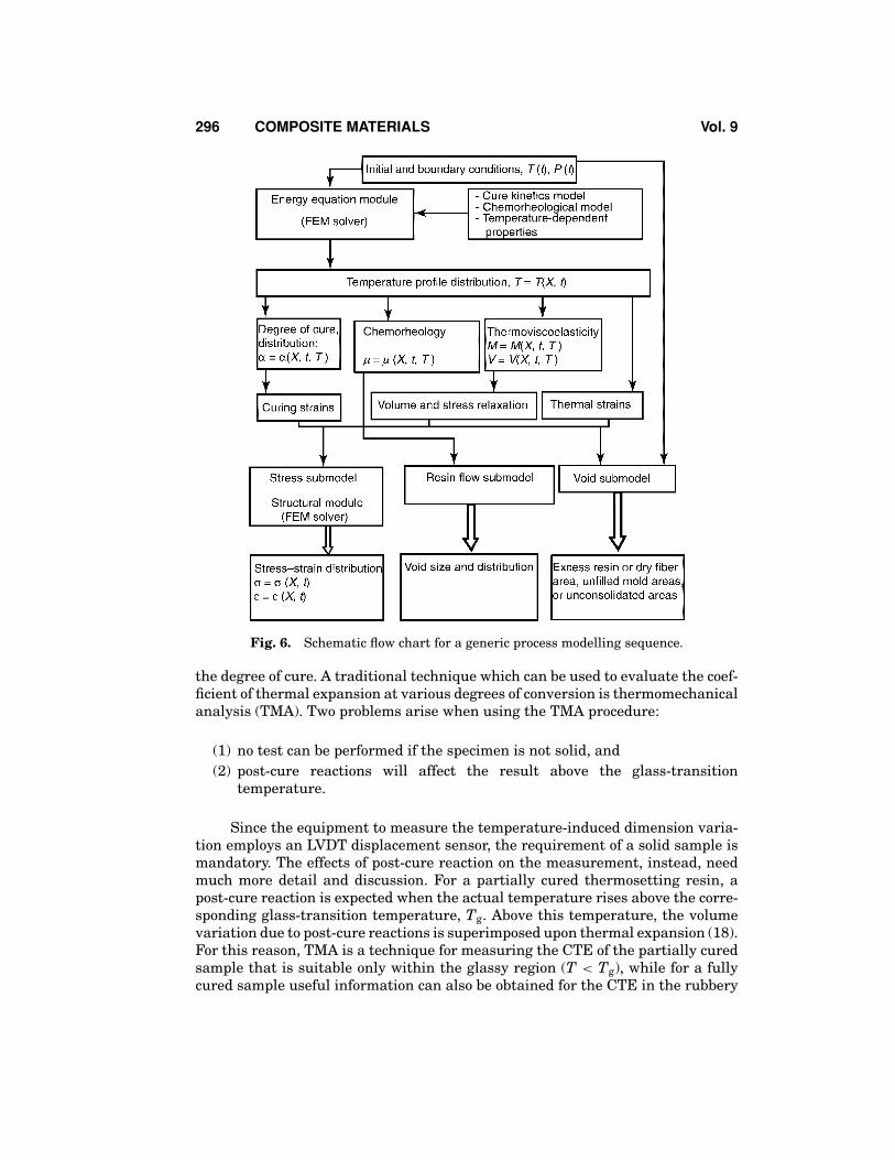
Fig. 5. Experimental matrix conversion profiles at different isothermal tempera-tures: , fitting; ◦, 180◦C (Exp) , 160◦C (Exp) �, 140◦C (Exp); •, 120◦C (Exp).


Fig. 6. Schematic flow chart for a generic process modelling sequence.

the degree of cure. A traditional technique which can be used to evaluate the coef-ficient of thermal expansion at various degrees of conversion is thermomechanicalanalysis (TMA). Two problems arise when using the TMA procedure:

(1) no test can be performed if the specimen is not solid, and(2) post-cure reactions will affect the result above the glass-transition

temperature.

Since the equipment to measure the temperature-induced dimension varia-tion employs an LVDT displacement sensor, the requirement of a solid sample ismandatory. The effects of post-cure reaction on the measurement, instead, needmuch more detail and discussion. For a partially cured thermosetting resin, apost-cure reaction is expected when the actual temperature rises above the corre-sponding glass-transition temperature, Tg. Above this temperature, the volumevariation due to post-cure reactions is superimposed upon thermal expansion (18).For this reason, TMA is a technique for measuring the CTE of the partially curedsample that is suitable only within the glassy region (T < Tg), while for a fullycured sample useful information can also be obtained for the CTE in the rubbery


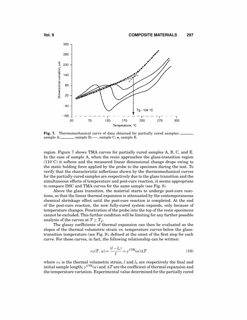
Fig. 7. Thermomechanical curve of data obtained for partially cured samples: ,sample A; , sample B;—–, sample C; •, sample E.

region. Figure 7 shows TMA curves for partially cured samples A, B, C, and E.In the case of sample A, when the resin approaches the glass-transition region(110◦C) it softens and the measured linear dimensional change drops owing tothe static holding force applied by the probe to the specimen during the test. Toverify that the characteristic inflections shown by the thermomechanical curvesfor the partially cured samples are respectively due to the glass transition and thesimultaneous effects of temperature and post-cure reaction, it seems appropriateto compare DSC and TMA curves for the same sample (see Fig. 8).

Above the glass transition, the material starts to undergo post-cure reac-tions, so that the linear thermal expansion is attenuated by the contemporaneouschemical shrinkage effect until the post-cure reaction is completed. At the endof the post-cure reaction, the now fully-cured system expands, only because oftemperature changes. Penetration of the probe into the top of the resin specimenscannot be excluded. This further condition will be limiting for any further possibleanalysis of the curves at T ≥ Tg.

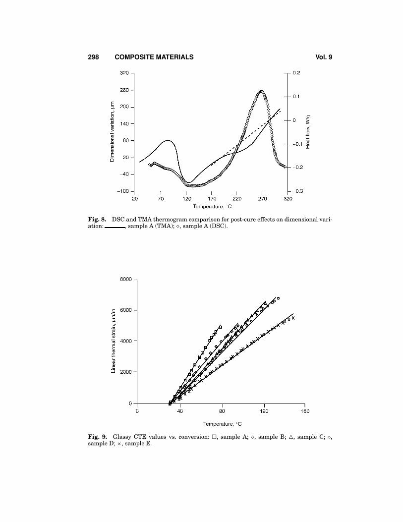
The glassy coefficients of thermal expansion can then be evaluated as theslopes of the thermal volumetric strain vs. temperature curves below the glass-transition temperature (see Fig. 9), defined at the onset of the first step for eachcurve. For these curves, in fact, the following relationship can be written:

εV(T, α) = (l − lo)l

= γ CTE(α) T (10)

where εV is the thermal volumetric strain, l and l0 are respectively the final andinitial sample length; γ CTE(α) and T are the coefficient of thermal expansion andthe temperature variation. Experimental value determined for the partially cured


Fig. 8. DSC and TMA thermogram comparison for post-cure effects on dimensional vari-ation: , sample A (TMA); �, sample A (DSC).

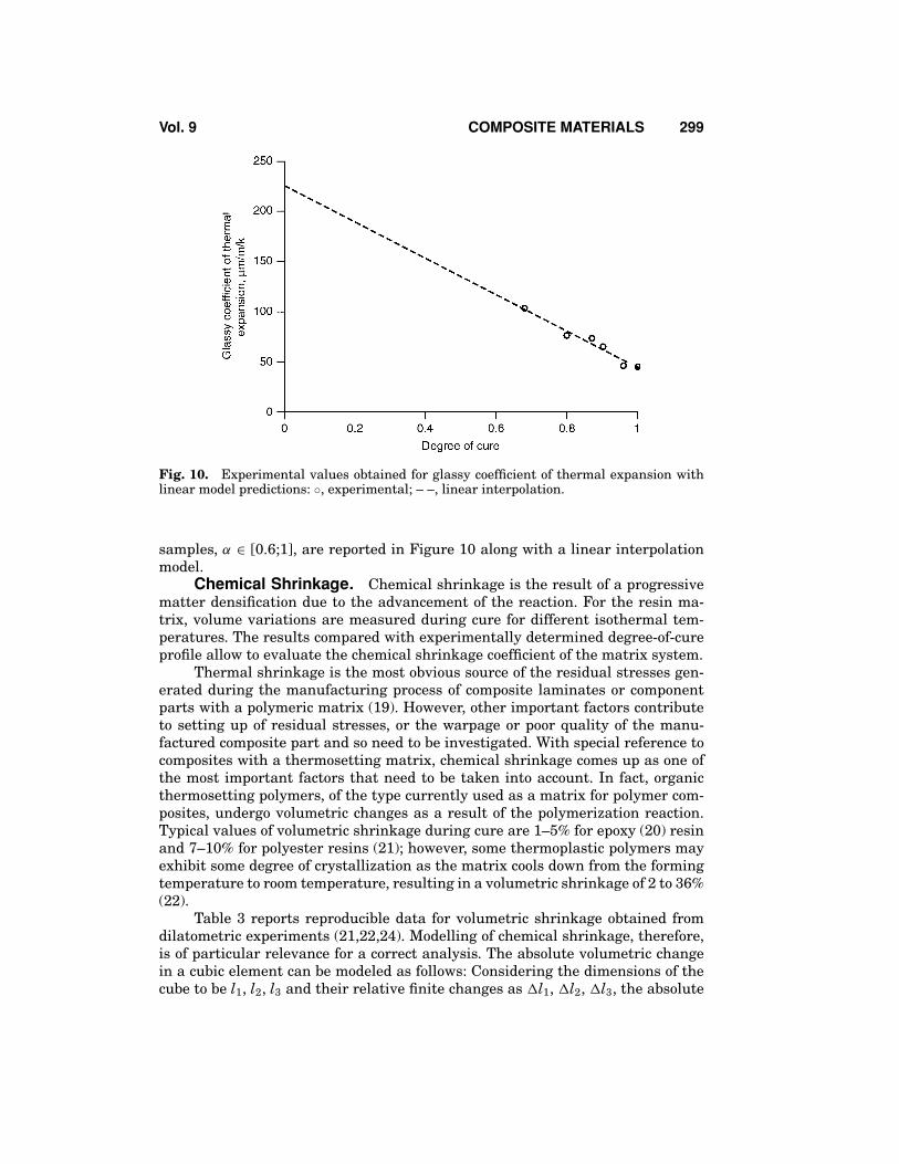
Fig. 9. Glassy CTE values vs. conversion: �, sample A; �, sample B; �, sample C; ◦,sample D; ×, sample E.


Fig. 10. Experimental values obtained for glassy coefficient of thermal expansion withlinear model predictions: ◦, experimental; – –, linear interpolation.

samples, α ∈ [0.6;1], are reported in Figure 10 along with a linear interpolationmodel.

Chemical Shrinkage. Chemical shrinkage is the result of a progressivematter densification due to the advancement of the reaction. For the resin ma-trix, volume variations are measured during cure for different isothermal tem-peratures. The results compared with experimentally determined degree-of-cureprofile allow to evaluate the chemical shrinkage coefficient of the matrix system.

Thermal shrinkage is the most obvious source of the residual stresses gen-erated during the manufacturing process of composite laminates or componentparts with a polymeric matrix (19). However, other important factors contributeto setting up of residual stresses, or the warpage or poor quality of the manu-factured composite part and so need to be investigated. With special reference tocomposites with a thermosetting matrix, chemical shrinkage comes up as one ofthe most important factors that need to be taken into account. In fact, organicthermosetting polymers, of the type currently used as a matrix for polymer com-posites, undergo volumetric changes as a result of the polymerization reaction.Typical values of volumetric shrinkage during cure are 1–5% for epoxy (20) resinand 7–10% for polyester resins (21); however, some thermoplastic polymers mayexhibit some degree of crystallization as the matrix cools down from the formingtemperature to room temperature, resulting in a volumetric shrinkage of 2 to 36%(22).

Table 3 reports reproducible data for volumetric shrinkage obtained fromdilatometric experiments (21,22,24). Modelling of chemical shrinkage, therefore,is of particular relevance for a correct analysis. The absolute volumetric changein a cubic element can be modeled as follows: Considering the dimensions of thecube to be l1, l2, l3 and their relative finite changes as l1, l2, l3, the absolute


Table 3. Shrinkage Measurements on Epon 828 Cured with Different Curing Agents,TETA and DTAa

Gel time, Volume shrinkage Total volumeSystem min after gelation % shrinkage

20 phr Triethylenetetramine(TETA), cure at 65◦C

116112110

2.312.292.34

5.72%/24 hr.5.72%/24 hr.5.79%/24 hr.

Diethylenetriamine 130130130

2.082.001.96

4.33 %/48 hr.4.33 %/48 hr.4.21 %/48 hr.

aFrom Ref. 23.

volume change is

| Vr| = Vfinal − Vinitial = [(l1 + l1)(l2 + l2)(l3 + l3)] − (l1l2l3) (11)

On dividing by the total unit volume of the element, equation 11 can beexpressed in terms of the strain components as follows:

Vr

Vr = ε1 + ε2 + ε3 + ε1ε2 + ε2ε3 + ε1ε3 + ε1ε2ε3 (12)

where εi for i = 1, 2, 3 represents the general strain component in the principaldirection.

Assuming that the volumetric shrinkage is isotropic, and neglecting allhigher order terms, the strain, εr corresponding to volume resin shrinkage,| Vr|, can be written as

εr = 12

(− 1 +

√(1 + 3

4 Vr

))(13)

Although dimensional changes are important in such operations as designingtooling for processing plastics or achieving the tolerances required in electronicand computing applications, and in encapsulating and laminating processes, thesedimensional changes are not as important in themselves as they are in determin-ing the stresses set up in the cured resin as a result of chemical shrinkage. Whenthese aspects of polymerization shrinkage are considered, it becomes apparentthat from the practical point of view the most important phase of the shrinkage topredict (and, hopefully, to control) is that occurring after gelation. If it is possible tolocate on the shrinkage/time curve the point of gelation, then data on shrinkageafter gelation become directly available. Shrinkage after gelation is minimizedwhen gelation occurs late in the curing reaction, since constrained conditions arisejust at the end of the curing process, thereby reducing the length of the crucialstage during which residual stresses can be set up. Lascoe (25) has reported a verycomprehensive study on the volume and linear shrinkage of an epoxy resin system.

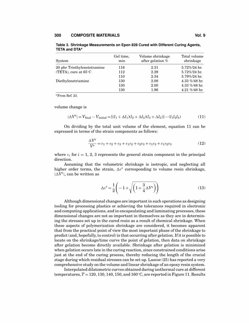
Interpolated dilatometric curves obtained during isothermal cure at differenttemperatures, T = 120, 130, 140, 150, and 160◦C, are reported in Figure 11. Results


Fig. 11. Linear interpolation of acquired data of specific volume variation during cure atdifferent isothermal temperatures.

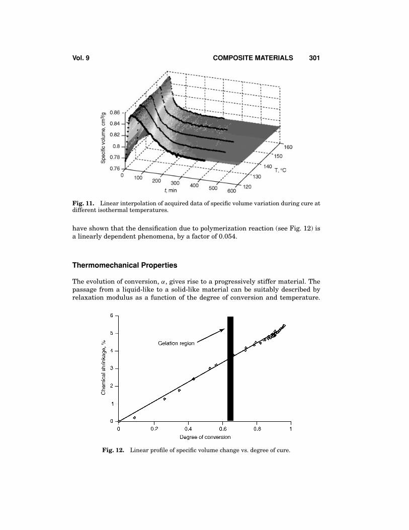
have shown that the densification due to polymerization reaction (see Fig. 12) isa linearly dependent phenomena, by a factor of 0.054.

Thermomechanical Properties

The evolution of conversion, α, gives rise to a progressively stiffer material. Thepassage from a liquid-like to a solid-like material can be suitably described byrelaxation modulus as a function of the degree of conversion and temperature.

Fig. 12. Linear profile of specific volume change vs. degree of cure.


Mapping the relaxation modulus in each body point then requires the experimen-tal evaluation of such quantity.

The data can be obtained from dynamic mechanical analysis (DMA) testsused to construct the stress relaxation master curves at different levels of con-version, within the frame of time-temperature superposition principle. Curvesof stress relaxation modulus can be modeled using the stretched Kohlrausch–William–Watts (KWW) exponential function at each level of conversion, as follows:

E(t, T, α) = E∞(α) exp[−(

ξ (t, T, α)τp(α)

)β(α)](14)

where E∞ indicates the fully relaxed modulus and τp and β are the KWW modelparameters. The functionality of the ultimate modulus and the KWW parametersover the degree of conversion is related to the physical assumption to consider as a“new material” the system at each level of conversion. A liner function was foundsatisfactory to model the nonexponential parameter β vs. conversion; Mijovic andco-workers (26) established the same linear dependency applied to dielectric con-stant decay function. Assuming that the molecular mobility influences the glasstransition through the same mechanism that controls the stress relaxation func-tion, then the behavior of the glass-transition temperature at a fixed degree ofcure can be normalized with respect of its value for a given conversion. This nor-malization will lead to the definition of a potential function, which is identicalto that obtained by normalizing in the same way the characteristic relaxationtimes with respect to the relaxation time at the same fixed conversion. From themathematical point of view, it can be stated that

Tg(α)Tg(αref)

= gTg (α) (15)

where Tg(α) is the glass-transition temperature as a function of the degree of cure,and Tg(αref) is the particular value for the fixed conversion. If the same mechanismdrives the change in normalized relaxation time, then it follows that

τp(α)τp(αref)

= gτp (α) (16)

and therefore,

gTg (α) = gτp (α) (17)

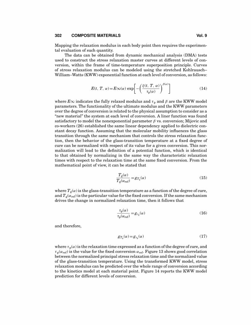
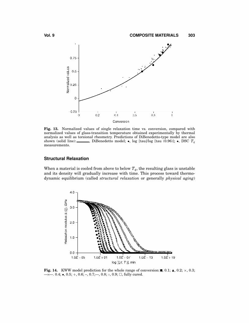
where τp(α) is the relaxation time expressed as a function of the degree of cure, andτp(αref) is the value for the fixed conversion αref. Figure 13 shows good correlationbetween the normalized principal stress relaxation time and the normalized valueof the glass-transition temperature. Using the transformed KWW model, stressrelaxation modulus can be predicted over the whole range of conversion accordingto the kinetics model at each material point. Figure 14 reports the KWW modelprediction for different levels of conversion.


Fig. 13. Normalized values of single relaxation time vs. conversion, compared withnormalized values of glass-transition temperature obtained experimentally by thermalanalysis as well as torsional rheometry. Predictions of DiBenedetto-type model are alsoshown (solid line): , DiBenedetto model; •, log [tau]/log [tau (0.96)]; •, DSC Tgmeasurements.

Structural Relaxation

When a material is cooled from above to below Tg, the resulting glass is unstableand its density will gradually increase with time. This process toward thermo-dynamic equilibrium (called structural relaxation or generally physical aging)

Fig. 14. KWW model prediction for the whole range of conversion: , 0.1; �, 0.2; ×, 0.3;—×—. 0.4; •, 0.5; +, 0.6; –, 0.7;—, 0.8; ◦, 0.9; �, fully cured.


occurs more rapidly at temperatures close to Tg, being an activated phenomenon,and manifests itself through a continuous change of a large number of propertiesincluding but not restricted to density, enthalpy, entropy, and consequently allthe related viscoelastic functions. The structural relaxation cannot be avoided;it occurs in all glasses even when cooling is performed such that the tempera-ture gradients over the material are small and the resulting thermal stresses arenegligible.

The structural relaxation is a direct consequence of the considerably longertime scale of molecular relaxations within and below the glass-transition regioncompared to the experimental time scale of the applied signal. In other words, eventhe slowest experimentally attainable cooling rate is much too fast for the polymerchains to relax to equilibrium. The nonequilibrium structure first experiences anabrupt contraction and then undergoes a time-dependent rearrangement towardthe equilibrium state. Monitoring the kinetics of any structure-sensitive propertychanges such as enthalpy or specific volume can follow the gradual rearrangementof the non-equilibrium structure. The multi-parameter phenomenological modelfor structural relaxation based on the Tool–Narayanaswamy–Mohinyan (TNM)theory was largely utilized in the literature for a number of organic and inorganicglasses.

In principle, the knowledge of TNM model parameters allows the predictionof volume as well as enthalpy relaxation under arbitrary thermal histories. Assuch, the volume as well as enthalpy fluctuations, which arise when polymersare cooled from the molten rubbery state, can be calculated at each body pointprovided the local thermal history is known.

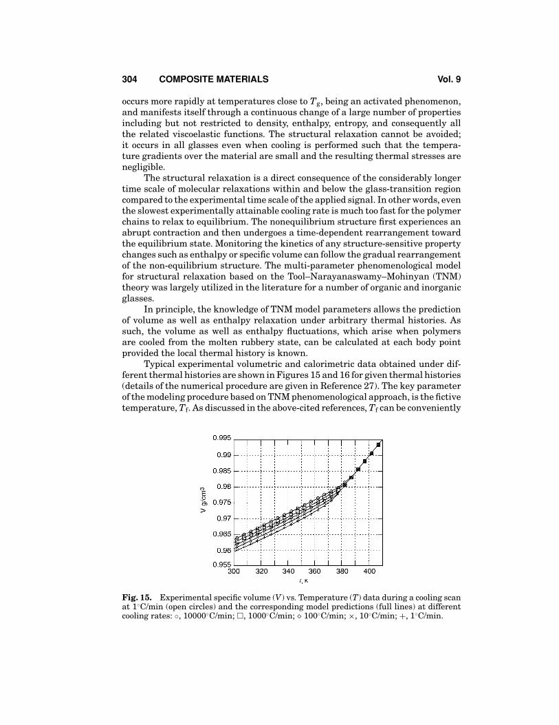
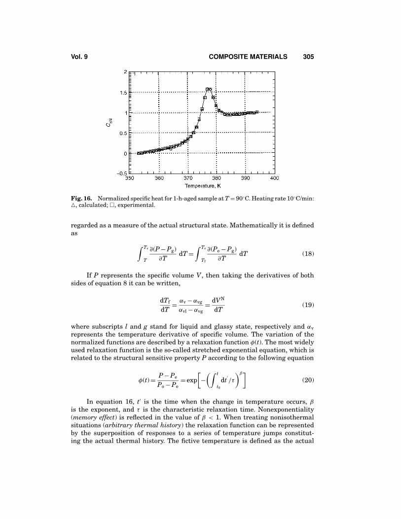
Typical experimental volumetric and calorimetric data obtained under dif-ferent thermal histories are shown in Figures 15 and 16 for given thermal histories(details of the numerical procedure are given in Reference 27). The key parameterof the modeling procedure based on TNM phenomenological approach, is the fictivetemperature, Tf. As discussed in the above-cited references, Tf can be conveniently

Fig. 15. Experimental specific volume (V) vs. Temperature (T) data during a cooling scanat 1◦C/min (open circles) and the corresponding model predictions (full lines) at differentcooling rates: ◦, 10000◦C/min; �, 1000◦C/min; � 100◦C/min; ×, 10◦C/min; +, 1◦C/min.


Fig. 16. Normalized specific heat for 1-h-aged sample at T = 90◦C. Heating rate 10◦C/min:�, calculated; �, experimental.

regarded as a measure of the actual structural state. Mathematically it is definedas

∫ Tr

T

∂(P − Pg)∂T

dT =∫ Tr

Tf

∂(Pe − Pg)∂T

dT (18)

If P represents the specific volume V, then taking the derivatives of bothsides of equation 8 it can be written,

dTf

dT= αv − αvg

αvl − αvg= dVN

dT(19)

where subscripts l and g stand for liquid and glassy state, respectively and αvrepresents the temperature derivative of specific volume. The variation of thenormalized functions are described by a relaxation function φ(t). The most widelyused relaxation function is the so-called stretched exponential equation, which isrelated to the structural sensitive property P according to the following equation

φ(t) = P − Pe

Po − Pe= exp

[−(∫ t

t0

dt′/τ

)β](20)

In equation 16, t′ is the time when the change in temperature occurs, β

is the exponent, and τ is the characteristic relaxation time. Nonexponentiality(memory effect) is reflected in the value of β < 1. When treating nonisothermalsituations (arbitrary thermal history) the relaxation function can be representedby the superposition of responses to a series of temperature jumps constitut-ing the actual thermal history. The fictive temperature is defined as the actual


non-equilibrium parameter and takes on the following form:

Tf (T) = T0 +∫ T

T0

{1 − exp

[−(∫ t(T)

t(T)dt/τ

)]}dT

′(21)

with T0 being the initial temperature. The next input needed by the model isan expression for the structural relaxation time τ , which appears in equation 6.Following Tool’s original work, various expressions for the structural relaxationtime have been proposed, all in exponential form and containing temperature andfictive temperature as variables.

The Narayanaswamy–Moynihan (NM) expression has the following form:

τ = A exp[x h∗

RT+ (1 − x)

h∗

RTf

](22)

where τ is the structural relaxation time, A is a constant (preexponential factor), h∗ is the characteristic activation energy, and x the partitioning parameter (0 <

x < 1) that defines the degree of nonlinearity.The experimental data of Figures 15 and 16 can be utilized to find the op-

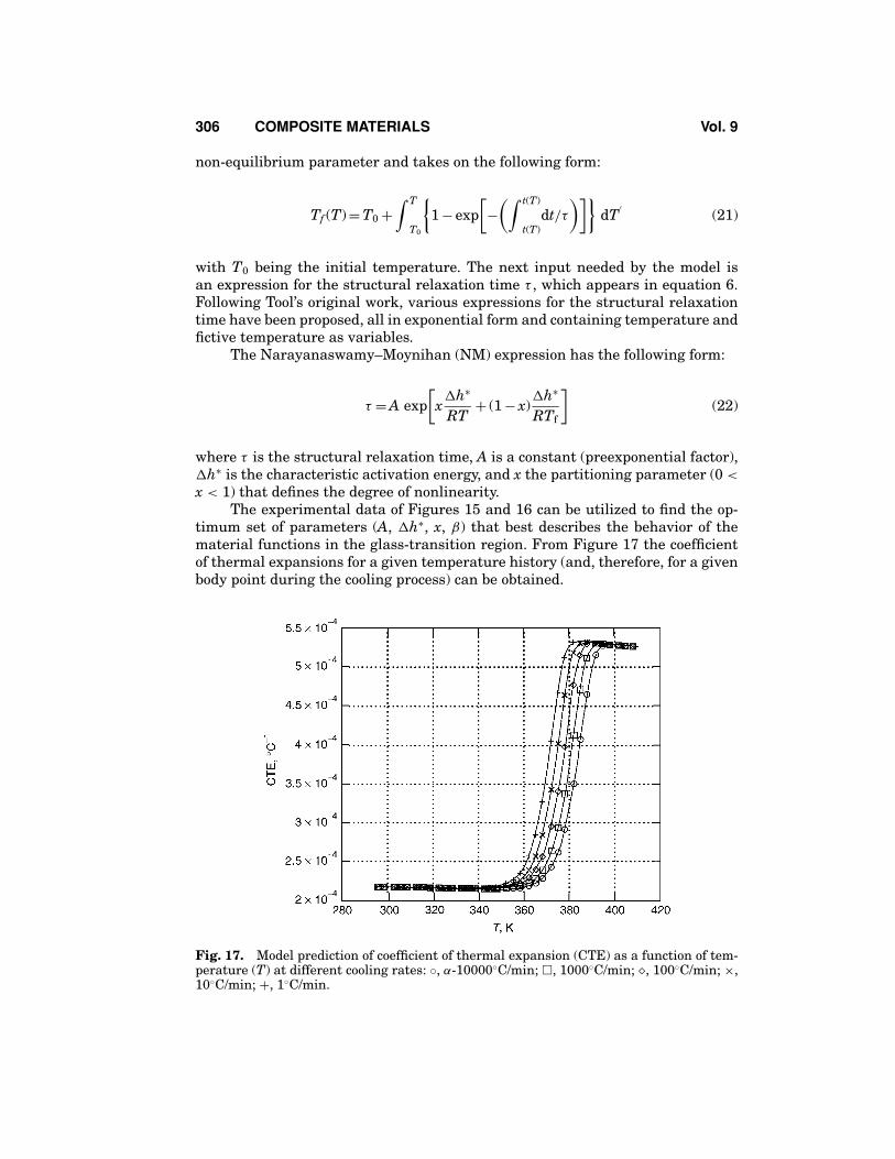
timum set of parameters (A, h∗, x, β) that best describes the behavior of thematerial functions in the glass-transition region. From Figure 17 the coefficientof thermal expansions for a given temperature history (and, therefore, for a givenbody point during the cooling process) can be obtained.

Fig. 17. Model prediction of coefficient of thermal expansion (CTE) as a function of tem-perature (T) at different cooling rates: ◦, α-10000◦C/min; �, 1000◦C/min; �, 100◦C/min; ×,10◦C/min; +, 1◦C/min.


Submodels

Resin Flow Submodel. Resin flow analysis in a manufacturing processprovides estimates of resin flow, and fiber and resin distribution and compaction.In the early stage of the autoclave process, after the prepregs are staked andvacuum bagged, the system is pressurized while the temperature is increasedin order to minimize the resin viscosity. In this way the resin flow removes theexcess resin from adjacent plies and makes uniform the fiber distribution. In theRTM process the dry fibers inside the mold can be considered as a porous mediumthrough which the resin is injected from a single or multiple inlets: Darcy’s lawcan be used to perform a two-dimensional flow analysis. Darcy’s law can be writtenas

[u(x, y)v(x, y)

]= − 1

µ

[kxx kxykyx kyy

]∂P(x, y)

∂x∂P(x, y)

∂y

(23)

where kij is the generic component of the permeability tensor, µ is the viscosity, Pis the pressure, and v and u are the components of the velocity in the x- and they-directions, respectively. If the resin is considered to be an incompressible fluidthen the continuity equation can be reduced to the following form:

∂u∂x

+ ∂v∂y

= 0 (24)

and the mass balance in an RTM process assumes the following form, provided thedirections x and y coincide with the principal directions of the fiber perform/mat(28).

∂

∂x

(kxx

µ

∂P∂x

)+ ∂

∂y

(kyy

µ

∂P∂y

)= 0 (25)

In autoclave forming the main resin flow is normal to the tool surface andDarcy’s law is again used but in its one-dimensional form:

V = − Sµ

dPdz

(26)

where S is the apparent permeability and z is the direction normal to the tool.Resin flow parallel to the tool plate takes place along the parallel and per-

pendicular fiber directions. Between the two mechanisms, the resin flow alongthe fibers is the most prominent as, in fact, the flow perpendicular to the fibers issmall because of the resistance created by the fibers.

The flow along the fiber direction can be modeled as a channel flow (theviscous flow between two parallel plates). Loss and Springer (29) validated ther-momechanical models, including the chemorheological behavior of resin and resinflow models.


Void Growth Model. The resin flow during composite processing in-evitably leads to the formation and growth of voids. Although all the manufac-turing processes of composite materials are based on solid engineering principles,current technologies cannot assure a part-by-part reliability required by the pro-duction and assembly of the parts for a complex and larger composite structure.For thick composite parts (30) the occurrence of voids has been widely verified andtheir detrimental effects proved. The void formation necessarily occurs during thefabrication process and involves the different concurrent phenomenology of heat,mass, and momentum transfer. An even more complex scenario comes out consid-ering that polymerization reaction occurs for the matrix while thermomechanicalproperties are varying with time, temperature, and degree of conversion. In somecases the system can be considered multiphase.

The correct mechanism of void formation is related to the system being usedand to the specific manufacturing process. Even when a part appears to be fullyimpregnated by the resin and the resin matrix has been previously degassed at theprescribed temperature, in order to eliminate mechanically entrapped air bubbles,void formation still occurs. During a general manufacturing process the voids canbe formed either by the mechanical entrapping of air or by a nucleation process. Inthe first case, it can be related to gas bubbles associated with the mixing operationof the resin bulk, by bridging of particles of additives, by air and wrinkles whenthe lay-up sequence is built, or by the resin flow during tow impregnation. Par-ticularly important for injection type processes (like RTM, injection molding, orresin film infusion) this latter mechanism leads to the formation of microvoids andconsequently dry spots within the low-permeability area of the perform. Schemat-ically, the voids formation associated with the resin flow can be divided in to fourstages, as follows:

(1) the flow reaches the tow to be impregnated,(2) the flow front comes around the tow or bundle and it passes,(3) still the resin has to penetrate and fill the space inside the tow among the

different fibers, and(4) air voids remain inside the tow and eventually move in the resin between

tows owing to the high pressure acting on the tow.

Modeling of void formation is intimately related with cure kinetics and vis-cosity profiles of the resin system. For modeling purposes it can be convenientlydivided into three different phases:

(1) formation and stability of the forming voids,(2) void growth and/or dissolution by diffusion, and(3) void transport process.

A nucleation process is generally described assuming the initial formationof the voids to be in accordance with the classical nucleation theory. It can beassumed that nucleation occurs between resin and fiber or resin and added particle(heterogeneous nucleation) or within the resin itself (homogeneous nucleation).


Application of classical nucleation theory (31) leads to favorable results, especiallyfor the case of homogeneous nucleation, for which critical size nuclei can be formedat rate N, given by the following equation:

N =[

PT

√2πMkT

]4π2 exp

(− F

kT

)(27)

where P stands for the total water plus air pressure, M is the molecular weightof the vapor phase, n the molecular density in the formed nuclei, F the max-imum free energy for the nucleation process, and k and T are respectively theBoltzmann constant and the absolute temperature. When the nuclei are formed,several factors determine the stability and the growth of the voids. Changes intemperature and pressure cause an increase in the solubility in the resin leadingto the dissolution of the voids. Generally, a void becomes stable when its innerpressure equals or exceeds the surrounding resin hydrostatic pressure plus thesurface tension forces. This condition can be stated as follows:

Pv − Psr = γr − v

Rv − a(28)

where Pv and Psr are respectively the void and resin pressure, λr − v is the resin–void surface tension, and Rv−a is the ratio of the volume and surface of the voids.As the temperature and pressure change with time, from a product-quality pointof view it is most important to model the time-dependent growth process.

This phenomenon, however, would require the solution of many time-dependent and coupled partial differential equations, which would result in toodifficult an approach. To overcome the intrinsic difficulties related to changesphysical properties and the excessive computational time of the equation solver,two “equivalent” physical schemes are generally studied assuming that the voidgrowth perpendicular to the ply (critical capillary scheme) or through an isotropicpseudo-homogeneous medium where the growth occurs not preferentially perpen-dicular to the plies. This latter approach seems to be more realistic considering thephysical possibility of pure water vapor growing for diffusion into the surroundingresin or into a void initially consisted of entrapped air and it become equivalentto bubble growth in a liquid medium.

The main assumptions in building a general void growth model are

(1) the voids remain between two plies and move with respect to the fixedcoordinates system in the laminate;

(2) the voids are considered spherical and their characteristic dimension iscalculated based on an equivalent sphere;

(3) no interactions between two voids are considered;(4) during the lay-up process and at the beginning of the cure process, void

nucleation occurs almost instantaneously;(5) temperature and moisture concentration are time independent; and(6) the void growth is limited by the flow rate of arrival of the diffusing species.


Structural Analysis

The complex interactions between material property evolution and the manufac-turing stages represent a critical issue for correct part design and for controllingthe entire production process. In order to evaluate the integrity of the manufac-tured part, a structural analysis needs to be performed to simulate the effects ofmechanical, nonmechanical, and geometric part constraints due to the manufac-turing tools utilized during the specific process.

Modeling of the coupled transfer phenomena (mass, heat, and momentum)need to be solved considering appropriate constitutive equations for the evolvingproperties in order to optimize the integrity of the final material system and atthe same time to control the final shape of produced composite element.

If, as we can recognize, the curing process involves thermal variations fromroom temperature to cure temperature, then thermal expansion is a necessarypart of that process. A common hypothesis has been proposed in past papers(32–36) to simplify the complex phenomenology, that is, no stresses develop priorto completion of the curing process.

Even if it is possible to obtain good results using a simulation model, in whichit is assumed that the crucial stage for formation of residual stresses is the periodof cooling from cure to ambient temperature, recent work has demonstrated thatthe residual stress formation mechanism is strongly influenced by the overall cur-ing process (37–43). Moreover, using this approach, the phenomenon of structuralrelaxation, which occurs near the glass-transition region of the developing struc-ture, is not considered at all. The above phenomena needs much more effort inorder to be well quantified and eventually taken into account. In fact, these chem-ical/physical changes cause more deformation in the transverse directions than inthe longitudinal direction since resin-dominant properties are experienced withinthe ply in that direction.

Mechanical Tests: Review

Mechanical tests for advanced composite materials conform in many respects tothe conventional test typology used for traditional isotropic materials. Despite thecomplication associated with the heterogeneity of composite systems, the interfacebetween fiber and matrix, and the anisotropy at the micro- and macroscopic lev-els, the same characteristic property definitions generally used for conventionalmaterials can be identified for these novel materials. In some cases additionalconstants are required and some differences in nomenclature are introduced es-pecially when no isotropic counterpart exists.

Mechanical characterization of composite materials is a complex scenario todeal with, either because of the infinite number of combinations of fiber and ma-trix that can be used, or because of the enormous variety of spatial arrangementsof the fibers and their volume content. The foundation of the testing methodsfor the measurement of mechanical properties is the classical lamination the-ory; this theory was developed during the nineteenth century for homogeneousisotropic materials and only later extended to accommodate features enhanced by


fiber-reinforced material, such as inhomogeneity, anisotropy, and anelasticity. Twobasic approaches are proposed to determine the mechanical properties of compos-ite materials: constituent testing and composite sample testing.

Academically, composite constituents could be tested separately and thencomposite properties evaluated by simple or more complex mixture rules accordingto the wanted level of accuracy. Many references can be found in the literature forthis approach. Mechanical properties of composites are generally assumed to bedependent on the following variables:

(1) properties of the fiber,(2) properties of the matrix,(3) properties of any other additive or phase constituting the composite,(4) volume fraction of the fiber,(5) spatial distribution of the fiber (or a third phase), and(6) nature of interface.

From a strictly theoretical point of view, the so-called constituent testingapproach or micromechanics approach is the most valuable. Tests performed oncomposite constituents supply the required material constants of each phase of thecomposite material—namely for long-fiber-reinforced composite—for the fiber andthe matrix, to use in appropriate mixture rules. These rules obtained by physicaland mechanical considerations are the basic relationships between the compositeconstituents, and they leads to a complete characterization of the final composite.

Fibers can be tested in the form of single fiber, tow, or fabric; all tests can begrouped into three main categories:

(1) Chemical Tests. They are generally used for elemental analysis and surfaceinvestigation. Following is a list of the most important chemical tests:

a. X-ray photoelectron spectroscopy (XPS)b. Low-energy electron diffraction (LEED)c. Scanning Electron Microscopy (SEM)d. Carbon assay (CA)e. Fourier transform infrared spectroscopy (FTIS)f. Sizing Content (SC)g. Thermal desorption mass spectrometry (TDMS)h. Auger electron spectroscopy (AES)

(2) Physical tests. They are generally performed to measure different physicalproperties for fiber and for fabric. Properties of interest required for specificapplication design are

a. Density (ASTM D792 using displacement, ASTM D3800 based onArchimedes principle and ASTM D1505 by means of density gradientcolumn)

b. Weight per length, typically in g/µmc. Weight per unit area or aerial weight, reported in g/m2


d. Filament diameter measured by microscopy image according to the stan-dard ASTM D578

e. Electrical conductivityf. Thermal expansiong. Number of twistsh. Tensile strength (ASTM D579)

(3) Mechanical test. It is important to point out that these mechanical testsare chosen based on whether the fiber sample is single fiber, tow, or fabric.For this reason, it is extremely important to define the specific fiber sampletypology used during the tests when a mechanical test campaign is started.The main mechanical tests generally performed are

a. Single-filament tensile test [ASTM D3379 (44)]b. Tensile test for tow [ASTM D4018 (45)]c. Tensile test for dry fabric [ASTM D579 (46)]

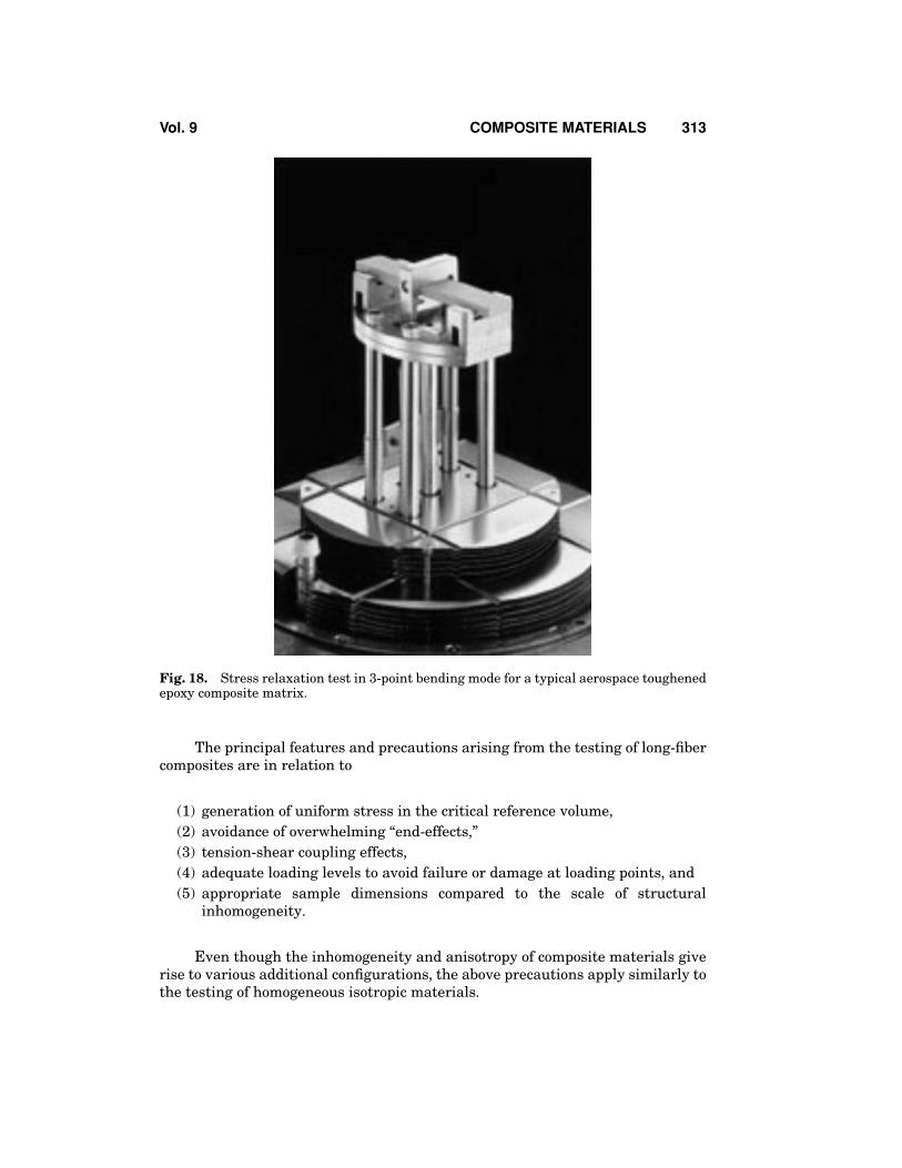
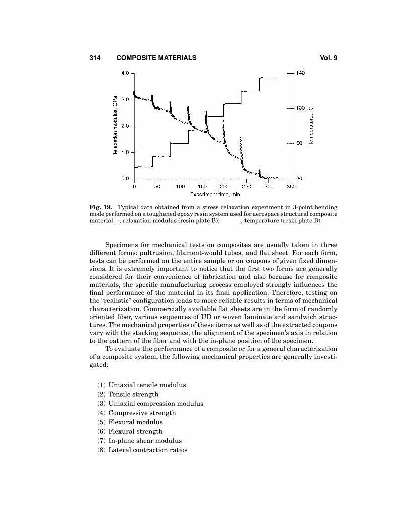
For resin matrix, several tests (chemical, physical, and mechanical) are gen-erally performed by the supplier; their results are used not only for design butalso for processing control and optimization. Along with traditional tests, somespecific procedures, such as stress relaxation or creep, are considered if viscoelas-tic effects are investigated. The experimental setup for the stress relaxation testis shown in Figure 18; while stress relaxation raw data, for an epoxy-toughenedresin matrix used for aerospace structural composite materials, are reported inFigure 19. Despite the fact that testing of a single constituent could eliminateinherent difficulties related with material handling, this approach is not repre-sentative of composite performance; in fact, many factors associated with the man-ufacturing process and the realistic arrangement of the fiber into the compositesystem are not taken into account as modeling assumptions are necessary evenin the case of more complex schematization.

The second approach, which determines the mechanical properties of thecomposites by directly testing a composite laminate, is a much more straightfor-ward procedure, widely implemented to determine composite properties requiredfor analysis and design. The whole philosophy of testing a laminate of compos-ite material is essentially based on the classical laminate theory. CLT employselasticity theory to derive the basic relationships between stress and strain and,therefore, to identify material properties. These relationships are quite simple fortraditional homogeneous and isotropic materials, however, for composites theycan be either extremely complex or, in some case, these equations are imperfect“tools” for modeling (ie it is not possible to estimate the stress state at the tip ofa crack by classical laminate theory). Static and fatigue tests are generally per-formed on composite laminates as well as on traditional systems; for these novelmaterials, however, some new test typologies need to be introduced to evaluatespecific properties or to describe particular failure modes not shown by traditionalmaterials. Despite inherent imperfections and simplifications, the existing formalframework contains justification for the various constraints and stipulations thathave been imposed on test configurations and procedures for long-fiber composites.


Fig. 18. Stress relaxation test in 3-point bending mode for a typical aerospace toughenedepoxy composite matrix.

The principal features and precautions arising from the testing of long-fibercomposites are in relation to

(1) generation of uniform stress in the critical reference volume,(2) avoidance of overwhelming “end-effects,”(3) tension-shear coupling effects,(4) adequate loading levels to avoid failure or damage at loading points, and(5) appropriate sample dimensions compared to the scale of structural

inhomogeneity.

Even though the inhomogeneity and anisotropy of composite materials giverise to various additional configurations, the above precautions apply similarly tothe testing of homogeneous isotropic materials.


Fig. 19. Typical data obtained from a stress relaxation experiment in 3-point bendingmode performed on a toughened epoxy resin system used for aerospace structural compositematerial: ◦, relaxation modulus (resin plate B); , temperature (resin plate B).

Specimens for mechanical tests on composites are usually taken in threedifferent forms: pultrusion, filament-would tubes, and flat sheet. For each form,tests can be performed on the entire sample or on coupons of given fixed dimen-sions. It is extremely important to notice that the first two forms are generallyconsidered for their convenience of fabrication and also because for compositematerials, the specific manufacturing process employed strongly influences thefinal performance of the material in its final application. Therefore, testing onthe “realistic” configuration leads to more reliable results in terms of mechanicalcharacterization. Commercially available flat sheets are in the form of randomlyoriented fiber, various sequences of UD or woven laminate and sandwich struc-tures. The mechanical properties of these items as well as of the extracted couponsvary with the stacking sequence, the alignment of the specimen’s axis in relationto the pattern of the fiber and with the in-plane position of the specimen.

To evaluate the performance of a composite or for a general characterizationof a composite system, the following mechanical properties are generally investi-gated:

(1) Uniaxial tensile modulus(2) Tensile strength(3) Uniaxial compression modulus(4) Compressive strength(5) Flexural modulus(6) Flexural strength(7) In-plane shear modulus(8) Lateral contraction ratios


Table 4. Mechanical Testing Plan for Mechanical Characterizationof Composite for Aeronautical Applications

Tensile strength at room temperatureUniaxial compression at room temperatureInterlaminar shear at room temperatureOpen hole tension at room temperature (see Fig. 19)Open hole compression at 93◦CHot/wet compression strengthEdge-plate compression strength after impact, at room temperature

(9) Apparent interlaminar shear strength(10) Facture toughness

With time, an extensive variety of test methods and procedures have beenintroduced to develop new applications of composite materials and more in gen-eral to sustain the diffusion in various fields of these novel materials. However,the complexity of the properties, the great variety of their applications, and the di-versity of their features compared with traditional materials have resulted in thedevelopments, often arbitrary and in some cases more specific, to satisfy particularsectors of the industry.

No single organization or industry is likely to carry out a general investi-gation program to identify a general routine procedure for mechanical character-ization of composite materials, supported by solid theoretical considerations. Inorder to satisfy the various downstream requirements, which vary from companyto company, different test programs have been stipulated. In USA, a large commer-cial airplane has proposed the test program reported in Table 4 as fundamentalfor the “initial” evaluation phase of composites, which differs from the test planidentified by U.S. automotive industries, whose test plan is reported in Table 5.

For composite materials, the exposure to critical environment is also an im-portant issue; therefore while selecting an appropriate test method for evaluat-ing composite mechanical properties the extreme conditions experienced duringservice for a particular application must be taken into account. Environmentalexposure can be “accidental” during the specimen preparation and instrumenta-tion, or “planned” to investigate the moisture effect, chemical attack, or cycling

Table 5. Mechanical Test Program Agreed by Important AutomotiveManufacturers

Elastic and strength properties at temperature in the range 40–150◦CEffect of loading rate on tensile and compressive properties

in the range 0.00167–16.7 s− 1

CreepCreep and stress relaxationResidual strength after fatigueFatigueEffects of notches and holesEnergy absorption after impactManufacturing effectsJoints and fastener characterization


temperature. In both cases, extensive and very expensive tests are performed toassess the performances of the composite material during service at these extremeconditions.

In 1987, a survey (47) of currently available mechanical standardized testsconcluded that the existing standardized, semistandardized, or available proce-dure were deficient in respect to three main aspects:

(1) too many variants were used for a single test and there was no evidence ofthe effects of the variation of generated data on reliability,

(2) some tests were not fit for their intended purpose, and(3) some important phenomena were neglected either because they were not

properly understood or because they were too time-consuming to assess.

The above-mentioned report has attributed this state of the art to poor inter-actions between academy and industry and to the failure to establish an adequatecommon infrastructure among composite experts and manufacturers. In the lastfew years, many laboratories in the area of composite materials have launchedinter-laboratory testing programs to establish common procedures for investiga-tion of mechanical properties by various techniques. Many round-robin test pro-grams (48–54) are still running in the area of interlaminar fracture mechanismon composite laminate fracture toughness of new 3-D-reinforced-fiber materials,dynamic mechanical analysis, through thickness crack propagation test, and fa-tigue tests. These research programs aim either to harmonize or to build a commonframework for parameters acquisition to be used for the analysis and design ofhigh quality composite structure.

Following is a list of the main testing mode adopted to characterize advancedcomposite materials along with reference standards:

(1) Tension: ASTM D3039, BS 2782-320, CRAG 300-301, CRAG 302, and ISO572

(2) Compression: ASTM D695M, ASTM 3400, and CRAG 400(3) Shear: ±45 tension test, 10◦ off-axis test, rail shear test, V-notched beam

test, plane-twist test, and torsion of thin-walled sample(4) Flexure: ASTM D790M-93, CRAG report 88012, BS2782-1005, and ISO

14125(5) Through-thickness testing: BS EN ISO 14 and 130, ASTM D3846, and

ASTM D 5379(6) Interlaminar fracture toughness(7) Impact: BS 2782, ASTM D3029-FA, ASTM 2930-FB, ISO/DIS 6603/2(8) Fatigue

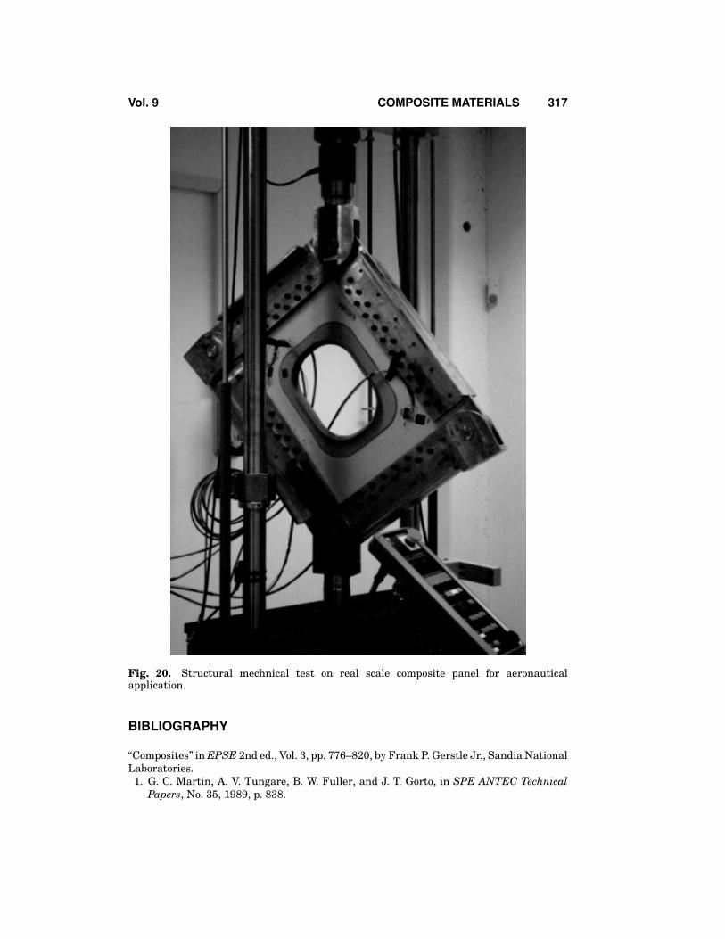
Structural tests on real-scale elements are also performed to validate thedesign criteria and manufacturing settings as a final verification of the desiredcomponents. In Figure 20, a typical test is shown for a real-scale composite panelfor aeronautical applications. The panel is loaded in shear mode under both staticand dynamic conditions.


Fig. 20. Structural mechnical test on real scale composite panel for aeronauticalapplication.

BIBLIOGRAPHY

“Composites” in EPSE 2nd ed., Vol. 3, pp. 776–820, by Frank P. Gerstle Jr., Sandia NationalLaboratories.

1. G. C. Martin, A. V. Tungare, B. W. Fuller, and J. T. Gorto, in SPE ANTEC TechnicalPapers, No. 35, 1989, p. 838.


2. E. Knauder, C. Kubla, and D. Poll, Kunstoffe German Plastics 81, 39 (1991).3. P. L. Chiou and A. Letton, Polymer 33, 3925 (1992).4. M. E. Ryan, M. Eng. Thesis, McGill University, Montreal, Canada, 1973.5. T. H. Hsieh and A. C. Su, J. Appl. Polym. Sci. 44, 165 (1992).6. C. D. Han and K. W. Lem, Polym. Eng. Sci. 24, 473 (1984).7. A. Hale, M. Gaircia, C. W. Macosko, and L. T. Manzione, in SPE ANTEC Technical

Papers, No. 35, 1989, p. 796.8. J. W. Lane and R. K. Khattacj, in SPE ANTEC Technical Papers, No. 33, 1987, p. 982.9. Y. S. Yang and L. Suspene, Polym. Eng. Sci. 31, 321 (1991).

10. A. Ya Malkin and S. G. Kulichikin, Adv. Polym. Sci. 101, 218 (1989).11. P. I. Karkanas, in Cure Modelling and Monitoring of Epoxy/Amine Resin Systems, PhD

Thesis, Cranfield University, United Kingdom, 1997.12. E. Rabinowitch, Trans. Faraday Soc. 33, 1225 (1937).13. S. L. Simon and J. K Gillham, J. Appl. Polym. Sci. 47, 461 (1993).14. J. D. Ferry, Viscoelastic Properties of Polymers, John Wiley & Sons, Inc., New York,

1976.15. Mita and K. Horie, J. Macromol. Sci. Rev. Macromol. Chem. Phys. C 27, 91 (1987).16. B. A. Rozenberg, Adv. Polym. Sci. 75, 113 (1988).17. A. T. DiBenedetto, J. Appl. Polym. Sci., Part B: Polym. Phys. 25, 1949 (1987).18. L. S. Penn, R. C. T. Chou, A. S. D. Wang, and W. K. Binienda, J. Comp. Mater. 23, 570

(1989).19. L. Di Palma, M. Bellucci, A. Apicella, P. Casone, M. Amato, and S. Rengo, in 32nd

International SAMPE Technical Conference, November 5–9, Boston, USA, 2000.20. C. T. Chou and L. S. Penn, J. Comp. Mater. 26(2), 171 (1992).21. E. J. Bartkus and C. H. Kroekel, Appl. Polym. Symp. 15, 113 (1970).22. T. J. Chapman, J. W. Gillespie, R. B. Pipes, J.-A. E. Manson, and J. C. Seferis, J. Comp.

Mater. 24, 616 (1990).23. H. L. Parry and H. A. Mackay, SPE J. 22 (1958).24. S. R. White and H. T. Hahn, J. Comp. Mater. 27, 1352 (1992).25. O. D. Lascoe, Eng. Tool 1, 32 (1958).26. M. Sun, Y. Han, and J. Mijovic, in Book of Abstracts of the International Conference on

“Time of Polymer” (TOP2002), Ischia, Italy, October 20–23, 2002.27. J. Mijovic, A. D’Amore, J. M. Kenny, and L. Nicolais, Polym. Eng. Sci. 34–35 (1994).28. S. K. Mazumdar, Composites Manufacturing: Materials Product and Process Engineer-

ing, CRC Press, Inc., Boca Raton, Fla., 2002.29. A. C. Loos and G. S. Springer, J. Comp. Mater. 17, 135 (1983).30. J. L. Kardos, M. P. Dudukovic, E. L. McKague, and M. W. Lehman, C. E. Browing, ed.,

Composite Materials: Quality Assurance and Processing, ASTM STP 797, AmericanSociety for Testing and Materials, Philadelphia, 1983.

31. W. D. Kingery, Introduction to Ceramics, John Wiley & Sons, Inc., New York, 1960.32. H. T. Hahn, J. Comp. Mater. 10, 266 (1976).33. H. Kau and L. A. Petrusha, Technical Report GMR-6359, G. M. Research Lab., Warren,

Mich., 1988.34. D. R. Doner and R. C. Novak, in 24th Annual Technical Conference (Paper No. 2), The

Society of Plastic Industry, 1969.35. O. H. Griffin, J. Comp. Mater. 17, 449 (1984).36. R. J. Stango and S. S. Wang, J. Eng. Ind. 106, 48 (1984).37. S. R. White and H. T. Hahn, J. Comp. Mater. 26, 2402 (1992).38. S. R. White and H. T. Hahn, J. Comp. Mater. 26, 2423 (1992).39. S.-Y. Lee and G. Springer, J. Comp. Mater. 22, 243 (1998).40. S. Y. Pusatcioglu and H. A. McGee Jr., J. Appl. Polym. Sci. 25, 381 (1980).41. T. A. Bogetti and J. W. Gillespie, J. Comp. Mater. 26, 262 (1992).

Vol. 9 COMPUTATIONAL CHEMISTRY 319

42. S. R. White and Y. K. Kim, Mech. Comp. Mater. Struct. 5, 153 (1998).43. K. S. Kim and H. T. Hahn, Comp. Sci. Technol. 36, 121 (1989).44. D3379, Annual Book of ASTM Standard, American Society for Testing and Materials,

Philadelphia.45. D4018, Annual Book of ASTM Standard, American Society for Testing and Materials,

Philadelphia.46. D579, Annual Book of ASTM Standard, American Society for Testing and Materials,

Philadelphia.47. P. J. Hoggs and S. Turner, “The mechanical testing of long-fibre composites: Harmo-

nization and standardization in U. K.”, Report of the Department of Trade and Industry,United Kingdom, January 1988.

48. G. D. Sims, “Standards for Polymer Matrix Composites. Part I: Assessment of CRAGTest Methods Data,” NPL Report DMM(M)6, 1990.

49. G. D. Sims, “International Standardisation of Coupon and Structural Element TestMethods,” in ECCM-Composites: Testing and Standardisation 2, Hamburg, 1994.

50. G. D. Sims and W. Nimmo, “A Review of Test Methods for Polymer Matrix Compositesat Non-Ambient Temperatures,” NPL Report DMM(A)155, 1994. (Summary available)

51. G. D. Sims, “Progress in Mechanical Behaviour and Testing Methods in CompositeMaterials,” in 5th Portuguese Congress on Fracture, Lisbon, 11–12 April 1994.

52. G. D. Sims, “Developments in Harmonisation of Standards for Polymer Matrix Com-posites,” in ECCM-Composites: Testing and Standardisation, Amsterdam, 1992.

53. G. D. Sims, Composites 22, 267–274 (1991).54. G. D. Sims, “Development of Standards for Advanced Polymer Matrix Composites—A

BPF/ACG Overview”, NPL Report DMM(A)8, (1990).

ALBERTO D’AMORE

The Second University of Naples—SUNMAURO ZARRELLI

Italian Aerospace Research Center

COMPOSITES, FABRICATION. See Volume 2.

Date post:	22-Mar-2018
Category:	Documents
Upload:	nguyendien
View:	231 times
Download:	1 times

'Composite Materials'. In: Encyclopedia of Polymer Science ...nguyen.hong.hai.free.fr/EBOOKS/SCIENCE...

Documents