Compositional Transient Stability Analysisof Multimachine Power Networks
Sina Yamac Caliskan and Paulo Tabuada
Abstract—During the normal operation of a power system, all thevoltages and currents are sinusoids with a frequency of 60 Hz inAmerica and parts of Asia or of 50 Hz in the rest of the world.Forcing all the currents and voltages to be sinusoids with the rightfrequency is one of the most important problems in power systems.This problem is known as the transient stability problem in thepower systems literature. The classical models used to study tran-sient stability are based on several implicit assumptions that areviolated when transients occur. One such assumption is the use ofphasors to study transients.While phasors require sinusoidal wave-forms to be well defined, there is no guarantee that waveforms willremain sinusoidal during transients. In this paper, we use energy-based models derived from first principles that are not subjectto hard-to-justify classical assumptions. In addition to eliminateassumptions that are known not to hold during transient stages, wederive intuitive conditions ensuring the transient stability of powersystems with lossy transmission lines. Furthermore, the conditionsfor transient stability are compositional in the sense that one inferstransient stability of a large power system by checking simpleconditions for individual generators.
Index Terms—Electromechanical systems, nonlinear controlsystems, power system dynamics, power system stability.
I. INTRODUCTION
P OWER system is the name given to a collection of devicesthat generate, transmit, and distribute energy to consuming
units such as residential buildings, factories, and street lighting.Abusing language, we use the terms power and energy inter-changeably, as typically done in the power systems literature.Excluding a small portion of generating units, such as solar cellsand fuel cells, we can think of power generators in a powersystem as electromechanical systems [3], [29]. Natural sources,such as the chemical energy trapped in fossil fuels, are used togenerate mechanical energy, which is then converted into elec-trical energy.
When power systems are working in normal operating con-ditions, i.e., in steady state, the generators satisfy two mainconditions: 1) their rotors rotate with the same velocity, whichis also known as synchronous velocity and 2) the generatedvoltages are sinusoidal waveforms with the same frequency.Keeping the velocity of the generators at the synchronousvelocity and the terminal voltages at the desired levels is called
frequency stability and voltage stability, respectively [22].Whenall the generators are rotating with the same velocity, they aresynchronized and the relative differences between the rotorangles remain constant. The ability of a power system to recoverand maintain this synchronism is called rotor angle stability.Transient stability, as defined in [22], is the maintenance of rotorangle stability when the power system is subject to large dis-turbances. These large disturbances are caused by faults on thepower system such as the tripping of a transmission line.
In industry, the most common way of checking transientstability of a power system is to run extensive time–domainsimulations for important fault scenarios [26]. This way ofdeveloping action plans for the maintenance of transient stabilityis easy and practical if we know all the “important” scenariosthatwe need to consider.Unfortunately, power systems are large-scale systems and the number of possible scenarios is quite large.As an exhaustive search of all of these scenarios is impossible,power engineers need to guess the important cases that theyneed to analyze. These guesses, as made by humans, are proneto errors. Moreover, time–domain simulations do not provideinsight for developing control laws that guarantee transientstability [27]. Because of these reasons, additional methods arerequired for transient stability analysis. Currently, the methodsthat do not rely on time–domain simulations can be collected intwo different groups: direct methods and automatic learningapproaches. The automatic learning approaches [38] are based onmachine learning techniques. In this work, we do not considerautomatic learning approaches and focus on direct methods.
A. Direct Methods and Their Limitations
Directmethods are based on obtainingLyapunov functions forsimplemodelsofpower systems [16], [26], [37].To thebestofourknowledge, theoriginof the idea canbe found in the1947paperofMagnusson [23], which uses the concept of “transient energy,”which is the sum of kinetic and potential energies to study thestability of power systems. In 1958, Aylett, assuming that a two-machine system can be represented by the dynamical equation
showed that thereexists aseparatrixdividing the two-dimensionalplane of and into two regions [2]. One of the regions is aninvariant set with respect to the two-machine system dynamics,i.e., if the initial condition is in this set, trajectories stay inside thisset for all future time. Aylett concluded that in order to check thestability of the system, we only need to check whether the state isin the invariant set or not. Aylett also characterized the separatrixthat defines the invariant set and extended the results from thetwo-machine case to the three-machine case in the same
Manuscript received September 20, 2013; revised September 23, 2013;accepted January 6, 2014. Date of publication February 5, 2014; date ofcurrent version April 9, 2014. This work was supported in part by theNational Science Foundation (NSF) award 1035916. Recommended byAssociate Editor C. Canudas-de-Wit.
The authors are with the Department of Electrical Engineering, University ofCalifornia, Los Angeles, CA 90095-1594 USA (e-mail: [email protected];[email protected]).
Color versions of one ormore of the figures in this paper are available online athttp://ieeexplore.ieee.org.
Digital Object Identifier 10.1109/TCNS.2014.2304868
4 TRANSACTIONS ON CONTROL OF NETWORK SYSTEMS, VOL. 1, NO. 1, MARCH 2014
monograph. Although the term “Lyapunov function” was notstated explicitly in hiswork,Aylett’swork usedLyapunov-basedideas. Some of the other pioneering works on direct methodsinclude Szendy [34], Gless [18], El-Abiad and Nagaphan [15],and Willems [39]. The work based on direct methods mainlyfocused on finding better Lyapunov functions that work for moredetailed models and provide less conservative results. TheseLyapunov functions are used to estimate the region of attractionof the stable equilibrium points that correspond to desiredoperating conditions. The stability of a power system after theclearance of a fault can then be tested by determiningwhether thepostfault state belongs to the desired region of attraction. Forfurther information, we refer the reader to [16], [26]–[28], and[37]. There are several problematic issues with direct methods.
The first problem is the set of assumptions used to constructthese models. The models used for transient stability analysisimplicitly assume that the angular velocities of the generators arevery close to the synchronous velocity. In other words, it isassumed that the system is very close to desired equilibrium andthe models developed based on this assumption are used toanalyze the stability of the same equilibrium. The standardanswer given to this objection is the following: the models thatare used in transient stability studies are used only for the “firstswing” transients and for these transients, the angular velocitiesof the generators are very close to the synchronous velocity.Unfortunately, in real-world scenarios, large swings need tobe considered. Citing the postmortem report [35, p. 25] ofAugust 14, 2003 blackout in Canada and the Northeast of theUnited States, “the large frequency swings that were inducedbecame a principal means by which the blackout spread across awide area.” Using models based on “first swing” assumptions toanalyze cases such as the August 14, 2003 blackout does notseem reasonable.
The second problem is that the models used for transientstability analysis, again implicitly, pose certain assumptions onthe grid. The transmission lines are modeled as impedances andthe loads are modeled either as impedances or as constant currentsources. These modeling assumptions are used to eliminate theinternal nodes of the network via a procedure called Kronreduction [3], [13]. The resulting network after Kron reductionis a strongly connected network. Every generator is connected toevery other generator via transmission lines modeled as a seriesconnection of an inductor and a resistor. After this reductionprocess, the resistances in the reduced grid are neglected. Thefundamental reason behind the neglect of the resistances lies inthe strong belief, in the power systems community, about thenonexistence of Lyapunov functions when these resistances arenot neglected. This belief stems from the paper [9], which assertsthe nonexistence of global Lyapunov functions for power sys-tems with losses in the reduced power grid model. It is furthersupported by the fact that the Lyapunov functions that the powersystems community has developed contain path-dependentterms unless these resistances are neglected. The reader shouldnote that the resistors here represent both the losses on thetransmission lines and the loads. Hence, this assumption impliesthat there is no load in the grid (other than the loads modeled ascurrent injections), which is not a reasonable assumption. Inaddition to these problems that have their origin in neglecting the
resistances on the grid, the process of constructing these reducedmodels, i.e., Kron reduction, can only be performed for a veryrestrictive class of circuits unless we assume that all the wave-forms in the grid are sinusoidal [4], [5]. In other words, in order toperform this reduction process for arbitrary networks, we need touse phasors, which in turn requires that all the waveforms in thegrid are sinusoidals and every generator in the power grid isrotating with the same velocity. This assumption is not compati-ble with the study of transients.
B. Control and Synchronization in Power Networks
Despite the long efforts to obtain control laws for powersystems with non-negligible transfer conductances, results onlyappeared in the beginning of the 21st century. For the singlemachine and the two-machine cases, a solution, under restrictiveassumptions, is provided in [25]. In the same work, the existenceof globally asymptotically stabilizing controllers for powersystems with more than two machines is also proved but noexplicit controller is suggested. An extension of the results in[25] to structure preserving models can be found in [10]. To thebest of our knowledge, the problem of finding explicit globallyasymptotically stabilizing controllers for power systems withnon-negligible transfer conductances and more than two gen-erators has only been recently solved in [7] and [8]. Although asolution has been offered for an important long-lasting problem,the models that are used in [8] are still the traditional models thatwe want to avoid in our work.
There are also some recent related results on synchronizationof Kuramoto oscillators [11], [12], [14]. If the generators aretaken to be strongly overdamped, these synchronization resultscan be used to analyze the synchronization of power networks.The synchronization conditions obtained in [11], [12], and [14]can also be used in certainmicrogrid scenarios [33]. In this paper,we provide results that do not require generators to be stronglyoverdamped.
C. A New Framework for Transient Stability of Power Systems
All the previously described methods use classical models forpower systems. They are only validwhen the generator velocitiesare very close to the synchronous velocity. In this paper, weabandon these models and use port-Hamiltonian systems [36] tomodel power systems from first principles. As already suggestedin [31], a power system can be represented as the interconnec-tion of individual port-Hamiltonian systems. There are severaladvantages of this approach. First, we have a clear understandingof how energy is moving between components. Second, we donot need to use phasors. Third, we do not need to assume all thegenerator velocities to be close to the synchronous velocity.Finally, using the properties of port-Hamiltonian systems, wecan easily obtain the Hamiltonian of the interconnected system,which is a natural candidate for a Lyapunov function. A similarframework, based on passivity, is being used in a research projecton the synchronization of oscillators with applications to net-works of high-power electronic inverters [30].
We first obtain transient stability conditions for generators inisolation from a power system. These conditions show that aslong as we have enough dissipation, there will be no loss of
CALISKAN AND TABUADA: COMPOSITIONAL TRANSIENT STABILITY ANALYSIS OF MULTIMACHINE POWER NETWORKS 5
synchronization. In [31], the port-Hamiltonian framework is alsoused to derive sufficient conditions for the stability of a singlegenerator. The techniques used in [31] rely on certain integra-bility assumptions that require the stator winding resistance to bezero. In contrast, our results hold for nonzero stator resistances.Moreover, while in [31], it is assumed that synchronous gen-erators have a single equilibrium; we show in this paper thatgenerators have, in general, three equilibria and offer necessaryand sufficient conditions on the generator parameters for theexistence of a single equilibrium. With the help of usefulproperties of port-Hamiltonian systems, we obtain sufficientconditions for the transient stability of the interconnected powersystem from the individual transient stability conditions for thegenerators. In addition to these sufficient conditions, whichwere also reported in [6], we provide a deeper discussion onthe modeling of synchronous generators and we also explainhow to relax the sufficient conditions with the help offlexible ACtransmission systems (FACTS) devices. Our results are impor-tant contributions for several reasons. First, we do not use thepreviously discussed questionable assumptions. Without theseassumptions, we can apply our conditions to realistic scenariosincluding cases with large frequency swings. Second, our resultsrelate dissipation with transient stability. This transparent rela-tion is hard to see in the classical framework due to shadowingassumptions. Third, we exploit compositionality to tame thecomplexity of analyzing large-scale systems.We propose simpleconditions that can be independently checked for each generatorwithout the need to construct a dynamical model for the wholepower system. Finally, extending our framework to more com-plex models is easier because we use port-Hamiltonian modelsfor the individual components. This flexibility will be helpful todesign future control laws for the generators.
II. NOTATIONS
We denote the diagonal matrix with diagonal elementsby and an -by- matrix of zeros
by . The vector R is denoted by , whereis its th element. The -by- identity matrix is denoted by .We say that R is positive semidefinite, denoted by
, if for all R . If, in addition to this, wealso have , only if , we call positive definite,denoted by > . Amatrix is negative semidefinite (definite),denoted by ( < ), if and only if is positive semi-definite (definite). The gradient of a scalar field with respect toa vector is given by .Note that the gradient is assumed to be a column vector. Considerthe affine control system
where M, U, and M is a manifold and U R is acompact set. The affine control system (1) has a port-Hamiltonianrepresentation if there exist smooth functions J M Rand R M R satisfying J J andR R for all M, and there exists a smoothfunction M R, which is called the Hamiltonian, such that
(1) can be written in the form
J R
The Hamiltonian can be thought of as the total energy of thesystem. The output of the port-Hamiltonian representation of (1) isgiven by
If we take the time derivative of the Hamiltonian, we obtain
R
The term in (3) represents the power supplied to thesystem. Therefore, property (3) states that the rate of increasein the Hamiltonian is less than the power supplied to thesystem. We refer to [36] for further details on port-Hamiltoniansystems.
III. SINGLE GENERATOR
In this section, we derive the equations of motion for a two-pole synchronous generator from first principles. The first step inthis derivation is to identify the Hamiltonian, the sum of thekinetic and the potential energy, of a single generator. We thenderive a stability condition, using theHamiltonian as a Lyapunovfunction, for the synchronous generator when the terminalvoltages are known. Although we only consider two-pole syn-chronous machines, the results in this section can easily begeneralized to machines with more than two poles.
A. Mechanical Model
Every synchronous generator consists of two parts: rotorand stator. Several torques act on the rotor shaft and cause therotor to rotate around its axis. Explicitly, we can write the torquebalance equation for the torques acting on the rotor shaft asfollows:
where is the rotor angle, is the moment of inertia of the rotorshaft, is the damping coefficient, is the applied mechanicaltorque, and is the electrical torque. The angular velocity of therotor shaft is . The total kinetic energy of the rotor can beexpressed as
Using the definition of the angular velocity , we can write (4)in the following form
6 TRANSACTIONS ON CONTROL OF NETWORK SYSTEMS, VOL. 1, NO. 1, MARCH 2014
Remark 1: In the classical power systems literature, the torquebalance equation (4) is scaled by . Defining ,
, , and and dividing both sidesof (4) by a constant value called rated power, the following set ofmechanical equations is obtained:
In these equations, the parameters and are assumed tobe constant, which implies that is either constant or slowlychanging. Equations (5) and (6) do not require such assumptionson .
B. Electrical Model
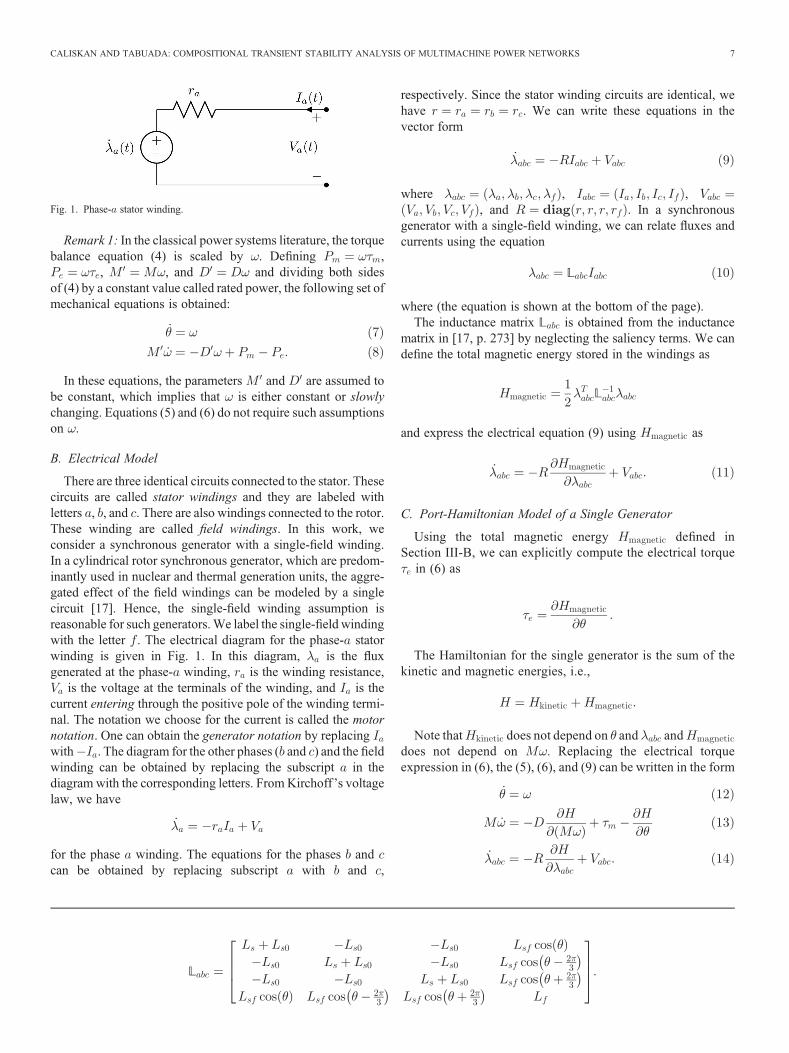
There are three identical circuits connected to the stator. Thesecircuits are called stator windings and they are labeled withletters , , and . There are also windings connected to the rotor.These winding are called field windings. In this work, weconsider a synchronous generator with a single-field winding.In a cylindrical rotor synchronous generator, which are predom-inantly used in nuclear and thermal generation units, the aggre-gated effect of the field windings can be modeled by a singlecircuit [17]. Hence, the single-field winding assumption isreasonable for such generators.We label the single-field windingwith the letter . The electrical diagram for the phase- statorwinding is given in Fig. 1. In this diagram, is the fluxgenerated at the phase- winding, is the winding resistance,
is the voltage at the terminals of the winding, and is thecurrent entering through the positive pole of the winding termi-nal. The notation we choose for the current is called the motornotation. One can obtain the generator notation by replacingwith . The diagram for the other phases ( and ) and the fieldwinding can be obtained by replacing the subscript in thediagram with the corresponding letters. FromKirchoff ’s voltagelaw, we have
for the phase winding. The equations for the phases andcan be obtained by replacing subscript with and ,
respectively. Since the stator winding circuits are identical, wehave . We can write these equations in thevector form
where , ,, and . In a synchronous
generator with a single-field winding, we can relate fluxes andcurrents using the equation
L
where (the equation is shown at the bottom of the page).The inductance matrix L is obtained from the inductance
matrix in [17, p. 273] by neglecting the saliency terms. We candefine the total magnetic energy stored in the windings as
L
and express the electrical equation (9) using as
C. Port-Hamiltonian Model of a Single Generator
Using the total magnetic energy defined inSection III-B, we can explicitly compute the electrical torque
in (6) as
The Hamiltonian for the single generator is the sum of thekinetic and magnetic energies, i.e.,
Note that does not depend on and anddoes not depend on . Replacing the electrical torqueexpression in (6), the (5), (6), and (9) can be written in the form
Fig. 1. Phase- stator winding.
L
CALISKAN AND TABUADA: COMPOSITIONAL TRANSIENT STABILITY ANALYSIS OF MULTIMACHINE POWER NETWORKS 7
If we define the energy variables , weobtain the port-Hamiltonian representation of (12)–(14) withstate , input , and
J R
D. Transformation from Domain to Domain and aSimplifying Assumption
Steady-state currents and voltages for the phases of thesingle generator are sinusoidal waveforms. In order to focus onthe simpler problem of stability of equilibrium points, weperform a change in coordinates R R defined by thepoint-wise linear map
with the inverse .
Remark 2: In the power systems literature, it is assumed thatthe generator rotor angles rotate with a speed that is very close tosynchronous speed , i.e., . If we integrate thisapproximation and assume zero initial conditions, we obtain
. When we replace in (15), the upper 3-by-3matrix of (15) becomes a transformation that maps balancedwaveforms with frequency to constant values, also known asPark’s transformation [29].
Using (15),we canmap -domain currentsto -domain currents . Notethat the field winding current is not affected by the changein coordinates. We define -winding voltages as
and -winding fluxes asin a similar fashion. We obtain
the Hamiltonian in the new coordinates as
L L
where L L is given by
L
Equations (12)–(14) can be written in the -domain as
J R
where and
J
At the desired steady-state operation, the fluxes are constantand is the synchronous velocity . Therefore, we can safelydisregard (17) and focus on the stability of the equilibria of (18).From the last row of (18), we have
which can be expressed in terms of currents as
by using the equality that follows fromL . Note that we can always design a control law
acting on the field winding terminals by choosing the voltageaccording to
for some < and a constant reference value . This controllerkeeps the field current constant and justifies the followingassumption:
Assumption 1: The field winding current is constant.If we use (10) and consider the field winding current to be
constant, we can express (18) in terms of currents
where and .
E. Equilibria of a Single Generator
In this section, we study the equilibria of a single generator.Recall that sinusoidal waveforms in the coordinates aremapped to constant values on the coordinates. Therefore,equilibria of (20)–(23) are points rather than sinusoidal trajecto-ries. We can find the equilibrium currents , , and thatsatisfy (21)–(23) when the voltages across the generator term-inals, , , and , are constant and equal to , , and ,respectively, by solving the algebraic equations
8 TRANSACTIONS ON CONTROL OF NETWORK SYSTEMS, VOL. 1, NO. 1, MARCH 2014
to obtain and
The values of are obtained by replacing (28) into thealgebraic equation obtained by setting in (20). This resultsin a third-order polynomial equation in . For any given R,if we choose
it is easy to show that one of the solutions of is .Therefore, we can always choose a torque value such that forany given steady-state inputs and desired synchro-nous velocity , one of the solutions of (20)–(23) is
with and given by (27) and (28), respectively, and .Note that in addition to , the equation has two othersolutions. For each solution, we potentially have an equilibriumpoint. Hence, in general, we have three equilibrium points. Byanalyzing the coefficients of the polynomial equation , it isnot difficult to show that the only real solution of is iff
<
where and are obtained by replacing with in (27) and(28), respectively. Inequality (31) is a necessary condition forglobal asymptotic stability of the equilibrium . In Section III-F,we obtain sufficient conditions by identifying constraints on thegenerator parameters that lead to a global Lyapunov function forthe equilibrium .
F. Stability of a Single Generator
In this section, we provide sufficient conditions for theequilibrium point computed in Section III-E to be globallyasymptotically stable. A natural choice for Lyapunov functioncandidate is the Hamiltonian of the single generator. How-ever, the minimum of occurs at the origin instead of
, where L . We shift the mini-mum of the Hamiltonian to by defining a function that we callthe shifted Hamiltonian. Explicitly, the shifted Hamiltonian isgiven as
L
We also define the shifted state by . It is easy tocheck that we have
where is the gradient of the Hamiltonian with respect to, evaluated at . Note that is positive definite andimplies , which in turn implies . Therefore, in orderto prove that is globally asymptotically stable, it is enough toshow that < , for . The time derivative of is given by
J R
From (18) and , we obtain
J R
J J R
J R
J J J R
where , and we used the equalityJ J J . From (34), we know that the term insideparentheses in (35) is equal to zero. Hence, (35) implies
J J J R
Taking the time derivative of the shifted Hamiltonian ,we get
J R
where . Note that the last element of is zerosince a constant field winding current implies .We can write the first term in the right-hand side of (37) as aquadratic function of . Explicitly,
CALISKAN AND TABUADA: COMPOSITIONAL TRANSIENT STABILITY ANALYSIS OF MULTIMACHINE POWER NETWORKS 9
where we used L to eliminate the flux variables.Replacing (38) in (37), we obtain
P
where
P
The eigenvalues of thematrixP are , ,and
Since we have , i.e., , if P is negativedefinite, then < , for . It is easy to check that if
<
holds, then < , which implies that the matrix P in (39) isnegative definite. Hence, if (41) holds, we have < , for ,which in turn implies that is globally asymptotically stable.We can summarize the preceding discussion in the followingresult.
Theorem 1: Let be an equilibrium point of the singlegenerator, described by (18) when we have and
. The equilibrium point is globallyasymptotically stable if
<
It is useful to express inequality (42) in terms of - and -axescurrents.We know that the -axis and -axis currents are differentfrom the traditional - and -axes currents during the transientstage. However, we haveat equilibrium. Thus, we can replace (42) with
< . Note that we are using motorreference directions. In order to find the generator currents, weneed to replace and by and , respectively. However,this change in reference directions does not affect (42). Condition(42) relates the total magnetic energy stored on the generatorwindings at steady state [left-hand side of (42)] to the dissipationterms and . This relation gives us a set of admissible steady-state currents in -coordinates (or alternatively, -coordinates)that lead to global asymptotical stability.
Remark 3: One can verify that if inequality (42) holds, theninequality (31) also holds while the converse is not true. This is tobe excepted since global asymptotical stability requires a uniqueequilibrium.
Remark 4: In the single machine infinite bus scenario, agenerator is connected to an infinite bus modeling the powergrid as a constant voltage source. The analysis of the singlemachine in this section, which is based on the assumption thatthe terminal voltages are constant, can also be seen as theanalysis of a single machine connected to an infinite bus. Inthe classical analysis of this scenario [1], there are multipleequilibrium points and energy-based conditions for localstability are obtained. The analysis in this section showsthat in fact a single equilibrium exists, under certainassumptions on the generator parameters, and that globalasymptotical stability is also possible. Such conclusions arenot possible to obtain using the classical models as they arenot detailed enough.
IV. STABILITY ANALYSIS OF MULTIMACHINE POWER SYSTEMS
A. Multimachine Power System Model
We consider a multimachine power system consisting ofgenerators, loads, and a transmission grid connecting thegenerators and the loads. We distinguish among different gen-erators by labeling each variable in the generator model with thesubscript . We make the following assumptionabout the multimachine power system.
Assumption 2: The transmission network can be modeled byan asymptotically stable linear port-Hamiltonian system withHamiltonian .
Concretely, this assumption states that whenever the inputsto the transmission network are zero, can be used as aquadratic Lyapunov function proving global asymptotic stabilityof the origin. Although it may appear strong, we note that it holdsinmany cases of interest. In particular, it is satisfiedwhenever weuse short- or medium-length approximate models to describetransmission lines in arbitrary network topologies. Furthermore,we discuss how it can be relaxed in Remark 5.
We denote the three-phase voltages across the load terminalsand currents entering into the load terminals by and ,respectively. Here, we use the letter to distinguish the currentsand voltages that correspond to a load from the ones thatcorrespond to a generator. The current entering into the loadterminals when we set is denoted by . Itfollows from the linearity assumption on the transmission net-work that we can perform an affine change in coordinates, so thatin the new coordinates, we have
where and are the input and the output of the port-Hamiltonian model, respectively, of the grid in the new coordi-nates with shifted Hamiltonian , ,and . Equation (43) represents an“incremental power balance,” i.e., a power balance in the shiftedvariables. Intuitively, it states that the net incremental powersupplied by the generators and the loads is equal to the netincremental power received by the transmission grid.
10 TRANSACTIONS ON CONTROL OF NETWORK SYSTEMS, VOL. 1, NO. 1, MARCH 2014
B. Load Models
We make the following assumption regarding loads.
Assumption 3: Each load is described by one of the followingmodels:
1) a symmetric three-phase circuit with each phase being anasymptotically stable linear electric circuit;
2) a constant current source.The proposed load models are quite simple and a subset of the
models is used in the power systems literature. It has recentlybeen argued [32] that the increase inDC loads, such as computersand appliances, interfacing the grid through power electronicsintensifies the nonlinear character of the loads. However, there isno agreement on how such loads should bemodeled. In fact, loadmodeling is still an area of research [24]. The first class of modelsin Assumption 3 contains the well-known constant impedancemodel in the power systems literature. Constant impedance loadmodels are commonly used in transient stability analysis [16] andcan be used to study the transient behavior of induction motors[17]. According to the IEEE Task Force on Load Representationfor Dynamic Performance, more than half of the energy gener-ated in the United States is consumed by induction motors [21].This observation, together with the fact that these three-phaseinduction motors can be modeled as three-phase circuits witheach phase being a series connection of a resistor, an inductor,and a voltage drop, justifies the constant impedance model usagein transient stability studies. The -circuit model suggested forinduction motors in [21] is also captured by Assumption 3. In[21], it is also stated that lighting loads behave as resistors incertain operational regions. This observation also suggests theusage of constant impedances for modeling the aggregatedbehavior of loads. The second load model in Assumption 3 isalso common in the power systems literature [24].
Any asymptotically stable linear electrical circuit has a uniqueequilibrium and admits a port-Hamiltonian representation withHamiltonian . By performing a change in coordinates, wecan obtain a port-Hamiltonian system for the shifted coordinateswith the shifted Hamiltonian satisfying
<
Let us now consider constant current loads. If a load drawsconstant current from the network, we have . Thisimplies and the contribution of the constant currentload to the incremental power balance (43) is zero. Thisobservation shows that we can neglect constant current loads,since they do not contribute to the incremental power balance.Therefore, in the remainder of the paper, we only consider thefirst type of loads in Assumption 3.
C. Stability of Multimachine Power Systems
Let be the shifted Hamiltonian for generator with respectto the equilibrium point , as defined in Sec-tion III-E. FromSection III-E,we know that for every generator ,we have
P
where P is a matrix obtained by adding subscript to theelements of the matrix P given by (40). Using the definitionsabove, we select our candidate Lyapunov function as
where is the shifted Hamiltonian of the transmission gridthat was introduced in Assumption 2 (Section IV-A). Ourobjective is to show that the equilibrium forthe generators is globally asymptotically stable. Note that everyequilibrium shares the same synchronous velocity . Hence,asymptotical stability of implies that all the generatorsconverge to the synchronous velocity . In addition to syn-chronize the generators’ angular velocity, we also need toensure that the currents flowing through the transmissionnetwork converge to preset values respecting several opera-tional constraints such as thermal limits of the transmissionlines. This will also be a consequence of asymptotical stabilityof the equilibrium . When this equilibrium is reached, thevoltages and currents at the generator terminals are and
, respectively. If we now regard the transmission networkand the loads as being described by an asymptotically stablelinear system driven by the inputs and , we realize thatall the voltages and currents in the transmission network andloads will converge to a unique steady state. We assume thatsuch steady state, uniquely defined by and , satisfiesall the operational constraints.
Taking the time derivative of , we obtain
P
where (47) follows from (3) and (48) follows from (43), (44),and (45). If
<
holds for , then P < for everyby Theorem 1. Therefore, if (49) holds for every ,we conclude from (48) that
P <
This only shows that is negative semidefinite. Since all oftheHamiltonians that constitute the total Hamiltonian havecompact level sets, the level sets of are also compact.Hence, we can apply La Salle’s Invariance Principle to conclude
CALISKAN AND TABUADA: COMPOSITIONAL TRANSIENT STABILITY ANALYSIS OF MULTIMACHINE POWER NETWORKS 11
that all the trajectories converge to the largest invariant setcontained in the set defined by
P
The left-hand side of (51) is a sum of negative definitequadratic terms (recall that P < ) and thus only zero when
for all . This implies , hence the generator states
globally asymptotically converge to if (50) holds. The pre-ceding discussion is summarized in the following result.
Theorem 2: Consider a multimachine power system withgenerators described by (18) with , and loadssatisfying Assumption 3 interconnected by a transmissionnetwork satisfying Assumption 2. Let be an equilibriumpoint for the generators that is consistent with all theequations describing the power system. The equilibrium isglobally asymptotically stable if
<
holds for all .Theorem 2 states that in order to check the stability of the
multimachine system, we only need to check a simple conditionfor each generator in the system. This makes our result compo-sitional in the sense that the complexity of condition (52) isindependent of the size of the network. All these conditions arebound together by and that obviously depend on the wholenetwork. However, the computation of the desired steady-statecurrents needs to be performed for reasons other than transientstability and thus are assumed to be readily available.
Remark 5: We note that if Assumption 2 is weakened fromasymptotic stability to stability of the transmission network, theequilibrium is still globally asymptotically stable. However,the voltages and currents in the transmission network are nolonger uniquely determined and may violate the operationalconstraints.
Inequality (52) is a sufficient condition for asymptoticstability. Typically, the stator winding resistance for eachgenerator is small, and inequality (52) is only satisfied for smallsteady-state currents. However, inequality (52) can be enforcedby actively controlling the voltage at the generator terminalsusing a static synchronous series compensator (SSSC), a FACTSdevice that is typically used for series compensation [19] of realand reactive power. Using an SSSC, we can introduce voltagedrops of , , and at thegenerator terminals without altering the current. The turn-on andturn-off times for the thyristors in an SSSC are at the level ofmicroseconds [19], small enough to enforce a voltage dropthat is a piece-wise constant approximation of ,
, and . The approximation error canalways be reduced by increasing the number of converter valvesin the SSSC. By repeating the stability analysis in this section,while considering this new voltage drop, we arrive at the relaxedcondition for global asymptotic stability
<
Since the power throughput of FACTS devices is in the orderof megawatts [19], we can choose a value for that is severalorders of magnitude larger than . Therefore, the relaxedinequality (53) allows for large steady-state currents and iswidely applicable to realistic examples.
V. SIMULATION
In this section, we apply our results to the two-generator single-load scenario depicted in Fig. 2. The generators are connected tothe load via transmission lines with impedances
. The load impedance is .We use the generator parameters provided in [29, Table 7.3].Using the provided values, the damping coefficients areselected as MVAs andMVAs as was done in [29, Example 7.1]. The stator windingresistances for the generators are taken to be .Using the values for and provided in [29, Table 7.3], weobtain and from the equations
. Since the parameters and cannot beobtained from [29, Table 7.3], we assume and
. The steady-state phase voltages are, , , and. The steady-state phase currents satisfying
the circuit constraints are , ,, and . The mechanical torques
and field winding currents are selected so as to be consistentwith these steady-state values. For bothgenerators, (31) is satisfiedwith this choice of parameters and the equilibrium is unique.We now investigate global asymptotic stability for this example.Condition (52) does not hold, since the winding resistancesfor the generators are zero and this leads to
< for . In orderto use the relaxed condition (53), we connect a SSSC in serieswith the generator terminals providing the voltage drops
, , and in phases ,, and , respectively. Condition (53) holds for generator if
>
Replacing the generator parameters into this inequality, weobtain > and > . We choose
to satisfy these inequalities and provideenough damping.
We numerically simulated the dynamics of the circuit in Fig. 2 toobtain the transient behavior following the occurrence of a fault.Without conjecturing anything about the nature of the fault or theprefault circuit, we simply assumed that the initial condition for the
Fig. 2. Two-generator single-load scenario.
12 TRANSACTIONS ON CONTROL OF NETWORK SYSTEMS, VOL. 1, NO. 1, MARCH 2014
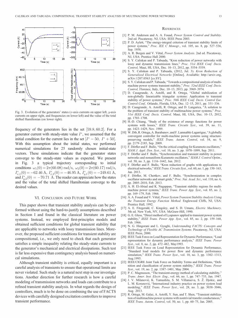
frequency of the generators lies in the set . For agenerator current with steady-state value , we assumed that theinitial condition for the current lies in the set .With this assumption about the initial states, we performednumerical simulations for 25 randomly chosen initial-statevectors. These simulations indicate that the generator statesconverge to the steady-state values as expected. We presentin Fig. 3 a typical trajectory corresponding to initialconditions , ,
, , ,and . The reader can appreciate how the statesand the value of the total shifted Hamiltonian converge to thedesired values.
VI. CONCLUSION AND FUTURE WORK
This paper shows that transient stability analysis can be per-formed without using the hard-to-justify assumptions describedin Section I and found in the classical literature on powersystems. Instead, we employed first-principles models andobtained sufficient conditions for global transient stability thatare applicable to networks with lossy transmission lines. More-over, the proposed sufficient conditions for transient stability arecompositional, i.e., we only need to check that each generatorsatisfies a simple inequality relating the steady-state currents tothe generator’s mechanical and electrical dissipations. Such testis far less expensive than contingency analysis based on numeri-cal simulations.
Although transient stability is critical, equally important is acareful analysis of transients to ensure that operational limits arenever violated. Such study is a natural next step in our investiga-tions. Another direction for further research is how a carefulmodeling of transmission networks and loads can contribute to arefined transient stability analysis. In what regards the design ofcontrollers, much is to be done on combining the use of FACTSdevices with carefully designed excitation controllers to improvetransient performance.
REFERENCES
[1] P. M. Anderson and A. A. Fouad, Power System Control and Stability.2nd ed. Piscataway, NJ, USA: IEEE Press 2003.
[2] P. D. Aylett, “The energy-integral criterion of transient stability limits ofpower systems,” Proc. IEE C Monogr., vol. 105, no. 8, pp. 527–536,Sep. 1958.
[3] A. R. Bergen and V. Vittal, Power System Analysis. 2nd ed. Piscataway,NJ, USA: Prentice Hall 2000.
[4] S. Y. Caliskan and P. Tabuada, “Kron reduction of power networks withlossy and dynamic transmission lines,” Proc. 51st IEEE Conf. Decis.Control, Maui, HI, USA, Dec. 10–13, 2012, pp. 5554–5559.
[5] S. Y. Caliskan and P. Tabuada, (2012, Jul. 3). Kron Reduction ofGeneralized Electrical Networks [Online]. Available: http://arxiv.org,arXiv:1207.0563 [cs.SY].
[6] S. Y. Caliskan and P. Tabuada, “Towards a compositional analysis of multi-machine power systems transient stability,” Proc. 52nd IEEE Conf. Decis.Control, Florence, Italy, Dec. 10–13, 2013, pp. 3969–3974.
[7] D. Casagrande, A. Astolfi, and R. Ortega, “Global stabilization ofnon-globally linearizable triangular systems: Application to transientstability of power systems,” Proc. 50th IEEE Conf. Decis. Control Eur.Control Conf., Orlando, Florida, USA, Dec. 12–15, 2011, pp. 331–336.
[8] D. Casagrande, A. Astolfi, R. Ortega, and D. Langarica, “A solution tothe problem of transient stability of multimachine power systems,” Proc.51st IEEE Conf. Decis. Control, Maui, HI, USA, Dec. 10–13, 2012,pp. 1703–1708.
[9] H.-D. Chiang, “Study of the existence of energy functions for powersystems with losses,” IEEE Trans. Circuits Syst., vol. 39, no. 11,pp. 1423–1429, Nov. 1989.
[10] W.Dib, R.Ortega,A.Barabanov, and F. Lamnabhi-Lagarrigue, “Agloballyconvergent controller for multi-machine power systems using structure-preserving models,” IEEE Trans. Autom. Control, vol. 54, no. 9,pp. 2179–2185, Sep. 2009.
[11] F. Dörfler and F. Bullo, “On the critical coupling for Kuramoto oscillators,”SIAM J. Appl. Dyn. Syst., vol. 10, no. 3, pp. 1070–1099, Sep. 2011.
[12] F. Dörfler and F. Bullo, “Synchronization and transient stability in powernetworks and nonuniform Kuramoto oscillators,” SIAM J. Control Optim.,vol. 50, no. 3, pp. 1116–1642, Jun. 2012.
[13] F. Dörfler and F. Bullo, “Kron reduction of graphs with applications toelectrical networks,” IEEETrans. Circuits Syst., vol. 60, no. 1, pp. 150–163,Jan. 2013.
[14] F. Dörfler, M. Chertkov, and F. Bullo, “Synchronization in complexoscillator networks and smart grids,” Proc. Nat. Acad. Sci., vol. 110, no. 6,pp. 2005–2010, Feb. 2013.
[15] A. H. El-Abiad and K. Nagappan, “Transient stability regions for multi-machine power systems,” IEEE Trans. Power App. Syst., vol. 85, no. 2,pp. 169–179, Feb. 1966.
[16] A. A. Fouad andV. Vittal,Power System Transient Stability Analysis Usingthe Transient Energy Function Method. Englewood Cliffs, NJ, USA:Prentice Hall, 1992.
[17] A. E. Fitzgerald, C. Kingsley, and S. D. Umans, Electric Machinery.5th ed. New York, NY, USA: McGraw-Hill, 1990.
[18] G. E. Gless, “Direct method of Lyapunov applied to transient power systemstability,” IEEE Trans. Power App. Syst., vol. 85, no. 2, pp. 159–168,Feb. 1966.
[19] N. G. Hingorani and L. Gyughi, Understanding FACTS: Concepts andTechnology of Flexible AC Transmission Systems. Piscataway, NJ, USA:IEEE Press, 2000.
[20] IEEETask Force on Load Representation for Dynamic Performance, “Loadrepresentation for dynamic performance analysis,” IEEE Trans. PowerSyst., vol. 8, no. 2, pp. 472–482, May1993.
[21] IEEE Task Force on Load Representation for Dynamic Performance,“Standard load models for power flow and dynamic performancesimulation,” IEEE Trans. Power Syst., vol. 10, no. 3, pp. 1302–1313,Aug.1995.
[22] IEEE/CIGRE Joint Task Force on Stability Terms and Definitions, “Defi-nition and classification of power system stability,” IEEE Trans. PowerSyst., vol. 19, no. 2, pp. 1387–1401, May 2004.
[23] P. C. Magnusson, “The transient-energy method of calculating stability,”Trans. Amer. Inst. Electr. Eng., vol. 66, no. 1, pp. 747–755, Jan. 1947.
[24] J. V. Milanovic, K. Yamashita, S. M. Villanueva, S. Ž. Djokic, andL. M. Korunovic, “International industry practice on power system loadmodeling,” IEEE Trans. Power Syst., vol. 28, no. 3, pp. 3038–3046,Aug. 2013.
[25] R. Ortega, M. Galaz, A. Astolfi, Y. Sun, and T. Shen, “Transient stabiliza-tion ofmultimachine power systemswith nontrivial transfer conductances,”IEEE Trans. Autom. Control, vol. 50, no. 1, pp. 60–75, Jan. 2005.
Fig. 3. Evolution of the generators’ states ( -axis currents on upper left, -axiscurrents on upper right, and frequencies on lower left) and the value of the totalshifted Hamiltonian (on lower right).
CALISKAN AND TABUADA: COMPOSITIONAL TRANSIENT STABILITY ANALYSIS OF MULTIMACHINE POWER NETWORKS 13
[26] M. Pavella and P. G. Murthy, Transient Stability of Power Systems: Theoryand Practice. West Sussex, U.K.: Wiley, 1994.
[27] M. Pavella, D. Ernst, and D. Ruiz-Vega, “Transient stability of powersystems: A unified approach to assessment and control,” inKluwer’s PowerElectronics and Power Systems Series, M. A. Pai, Ed. Dordrecht,The Netherlands: Kluwer Academic Publishers, 2000.
[28] M. A. Pai, Energy Function Analysis for Power System Stability. Boston,MA, USA: Kluwer Academic Publishers, 1986.
[29] P. Sauer andM. A. Pai, Power SystemDynamics and Stability.Champaign,IL, USA: Stipes Publishing LLC, 1997.
[30] L. A. B. Torres, J. Hespanha, and J. Moehlis, “Synchronization ofoscillators coupled through a network with dynamics: A constructiveapproach with applications to the parallel operation of voltage power sup-plies,” Sep. 2013 [Online]. Available: http://www.ece.ucsb.edu/~hespanha,submitted.
[31] S. Fiaz, D. Zonetti, R. Ortega, J. M. A. Scherpen, and A. J. van der Schaft,“A port-Hamiltonian approach to power network modeling and analysis,”Eur. J. Control, vol. 19, no. 6, pp. 477–485, Dec. 2013.
[32] M. J. H. Raja, D.W. P. Thomas, andM. Sumner, “Harmonics attenuation ofnonlinear loads due to linear loads,” Proc. Asia-Pacific Symp. Electromag.Compatibility (APEMC), Singapore, May 21–24, 2012, pp. 829–832.
[33] J. W. Simpson-Porco, F. Dörfler, and F. Bullo, “Synchronization andpower-sharing for droop-controlled inverters in islanded microgrids,”Automatica, vol. 49, no. 9, pp. 2603–2611, Sep. 2013.
[34] K. Szendy, “Kriterium der dynamischen Stabilität in Dreigeneratorensyste-men und dessen Verallgemeinerung auf Mehrgeneratorensysteme,” Arch.Elektrotech., vol. XLVII. Band, 3. Heft, pp. 149–160, 1962.
[35] The United States Department of Energy, Interim Report: Causes of theAugust 14th Blackout in the United States and Canada, U.S.–CanadaPower System Outage Task Force, Nov. 2003.
[36] A. J. van der Schaft, -Gain and Passivity Techniques in NonlinearControl, Lecture Notes in Control and Information Sciences. vol. 218,Berlin/Heidelberg, Germany: Springer-Verlag, 1996.
[37] P. Varaiya, F. F.Wu, andR.-L. Chen, “Direct methods for transient stabilityanalysis for power systems: Recent results,” Proc. IEEE, vol. 73, no. 12,pp. 1703–1715, Dec. 1985.
[38] L. A. Wehenkel, Automatic Learning Techniques in Power Systems.Boston: Springer. 1998.
[39] J. L.Willems, “Direct methods for transient stability studies in power systemanalysis,” IEEE Trans. Automat. Control, vol. 16, no. 4, pp. 332–341,Aug. 1971.
SinaYamacCaliskanwas born inAnkara, Turkey, in1987. He received the B.S. degree from Orta DoguTeknik Universitesi [ODTÜ; Middle East TechnicalUniversity (METU)], Ankara, Turkey, in 2008, andthe M.S. degree from Bilkent University, Ankara,Turkey, in 2010. He is a Ph.D. candidate, workingunder the supervision of Prof. P. Tabuada, with theDepartment of Electrical Engineering, University ofCalifornia, Los Angeles, CA, USA. He is affiliatedwith the Cyber-Physical Systems Lab (CyPhyLab) atUniversity of California.
His research interests include control theory, power systems, and softwareverification/synthesis.
Paulo Tabuada was born in Lisbon, Portugal, 1 yearafter the Carnation Revolution. He received the“Licenciatura” degree inAerospace Engineering fromInstituto Superior Tecnico, Lisbon, Portugal, in 1998,and the Ph.D. degree in electrical and computerengineering from the Institute for Systems andRobotics, Lisbon, Portugal, a private research instituteassociated with Instituto Superior Tecnico, in 2002.Between January 2002 and July 2003, he was a
Postdoctoral Researcher at the University ofPennsylvania, Philadelphia, PA,USA.After spending
3 years at the University of Notre Dame as an Assistant Professor, he joinedthe Electrical Engineering Department, University of California, Los Angeles,CA, USA, where he established and directs the Cyber-Physical SystemsLaboratory. In 2009, he co-chaired the International Conference on HybridSystems: Computation and Control (HSCC’09), and in 2012, he was a ProgramCo-Chair of the 3rd IFAC Workshop on Distributed Estimation and Control inNetworked Systems (NecSys’12). He also served on the editorial board of theIEEE EMBEDDED SYSTEMS LETTERS and the IEEE TRANSACTIONS ON AUTOMATIC
CONTROL.Dr. Tabuada’s contributions to cyber-physical systems have been recognized
by multiple awards including the NSF CAREER award in 2005, the DonaldP. Eckman award in 2009, and the George S. Axelby award in 2011. His latestbook, on verification and control of hybrid systems, was published by Springer in2009.
14 TRANSACTIONS ON CONTROL OF NETWORK SYSTEMS, VOL. 1, NO. 1, MARCH 2014