1

Educational Chapter

Compressed Air Energy Storage

Trishna Das

James D. McCalley

Iowa State University

Ames, Iowa

2012

Copyright © Trishna Das, 2012. All rights reserved.

2

Contents LITERATURE REVIEW .................................................................................................................................. 3

SITES FOR CAES ......................................................................................................................................... 4

DRAWBACKS OF CAES ............................................................................................................................... 6

CAES - ADVANCED TECHNOLOGY OPTIONS ............................................................................................... 6

STATE SPACE MODEL OF CAES .................................................................................................................... 8

MODEL DESCRIPTION ................................................................................................................................. 8

MODEL VALIDATION WITH HUNTORF OPERATIONAL DATA ..................................................................... 10

PERFORMANCE & ECONOMIC CHARACTERIZATION ................................................................................ 12

Performance indices ............................................................................................................................ 12

Economic indices ................................................................................................................................ 13

NUMERICAL RESULTS .............................................................................................................................. 16

Simulation results for 220 mw caes .................................................................................................... 16

Effect of caes sizing on economics and performance ......................................................................... 19

Effect of pressure limits on economics and performance ................................................................... 22

ECONOMICS AND GRID BENEFITS EVALUATION USING PRODUCTION COSTING ..................................... 23

COMPRESSED ENERGY AIR STORAGE IN PRODUCTION COSTING MODEL ................................................. 23

UNIT COMMITMENT PROBLEM FORMULATION ........................................................................................ 27

ECONOMIC DISPATCH PROBLEM FORMULATION...................................................................................... 28

CASE STUDY ............................................................................................................................................ 28

Ancillary service requirements ........................................................................................................... 28

Results: caes operation analysis .......................................................................................................... 30

CONCLUSIONS .......................................................................................................................................... 33

BIBLIOGRAPHY ........................................................................................................................................... 34

3

Educational Chapter:

Compressed Air Energy Storage

LITERATURE REVIEW

Storage technologies promise a wide range of benefits to nation‘s power sector such as grid

optimization improvement for bulk power production, smooth out variable renewable energy sources,

alleviate investment planning to support meet peak demands, provide ancillary services [1]. In the wake

of drastic promotion of renewable energy, specifically wind farms, there is a growing interest in

identifying large capacity and fast responding storage options to smooth out slow and fast wind variations

respectively.

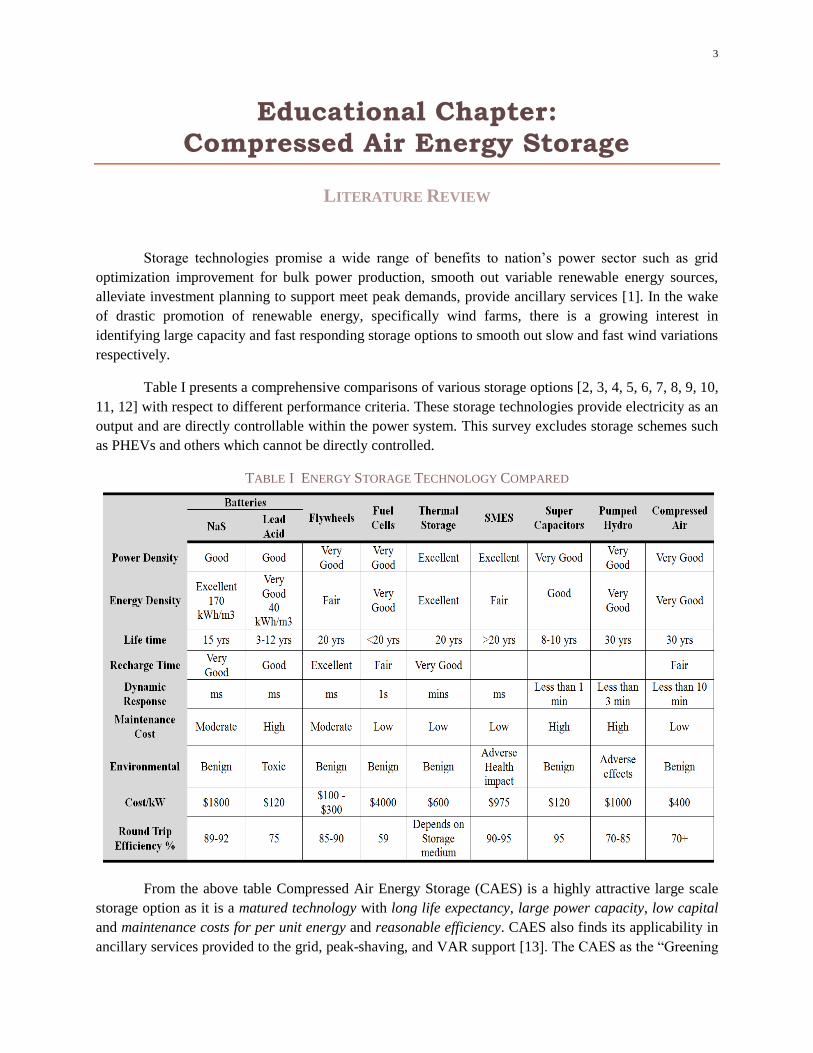
Table I presents a comprehensive comparisons of various storage options [2, 3, 4, 5, 6, 7, 8, 9, 10,

11, 12] with respect to different performance criteria. These storage technologies provide electricity as an

output and are directly controllable within the power system. This survey excludes storage schemes such

as PHEVs and others which cannot be directly controlled.

TABLE I ENERGY STORAGE TECHNOLOGY COMPARED

From the above table Compressed Air Energy Storage (CAES) is a highly attractive large scale

storage option as it is a matured technology with long life expectancy, large power capacity, low capital

and maintenance costs for per unit energy and reasonable efficiency. CAES also finds its applicability in

ancillary services provided to the grid, peak-shaving, and VAR support [13]. The CAES as the ―Greening

4

Technology‖ [14] is expected to address the variability of wind energy by performing load leveling,

ramping and frequency regulation, reducing or eliminating wind spillage.

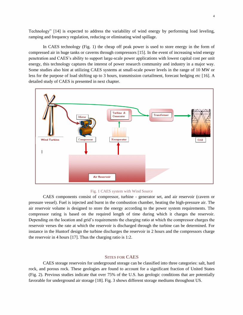
In CAES technology (Fig. 1) the cheap off peak power is used to store energy in the form of

compressed air in huge tanks or caverns through compressors [15]. In the event of increasing wind energy

penetration and CAES‘s ability to support large-scale power applications with lowest capital cost per unit

energy, this technology captures the interest of power research community and industry in a major way.

Some studies also hint at utilizing CAES systems at small-scale power levels in the range of 10 MW or

less for the purpose of load shifting up to 3 hours, transmission curtailment, forecast hedging etc [16]. A

detailed study of CAES is presented in next chapter.

Fig. 1 CAES system with Wind Source

CAES components consist of compressor, turbine - generator set, and air reservoir (cavern or

pressure vessel). Fuel is injected and burnt in the combustion chamber, heating the high-pressure air. The

air reservoir volume is designed to store the energy according to the power system requirements. The

compressor rating is based on the required length of time during which it charges the reservoir.

Depending on the location and grid‘s requirements the charging ratio at which the compressor charges the

reservoir verses the rate at which the reservoir is discharged through the turbine can be determined. For

instance in the Huntorf design the turbine discharges the reservoir in 2 hours and the compressors charge

the reservoir in 4 hours [17]. Thus the charging ratio is 1:2.

SITES FOR CAES

CAES storage reservoirs for underground storage can be classified into three categories: salt, hard

rock, and porous rock. These geologies are found to account for a significant fraction of United States

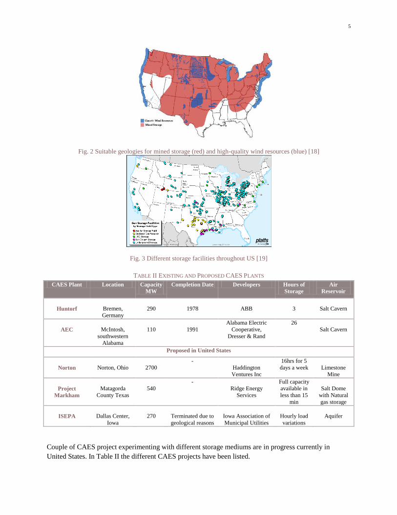
(Fig. 2). Previous studies indicate that over 75% of the U.S. has geologic conditions that are potentially

favorable for underground air storage [18]. Fig. 3 shows different storage mediums throughout US.

Wind Turbine

Air Reservoir

5

Fig. 2 Suitable geologies for mined storage (red) and high-quality wind resources (blue) [18]

Fig. 3 Different storage facilities throughout US [19]

TABLE II EXISTING AND PROPOSED CAES PLANTS

CAES Plant Location Capacity

MW

Completion Date Developers Hours of

Storage

Air

Reservoir

Huntorf

Bremen,

Germany

290

1978

ABB

3

Salt Cavern

AEC

McIntosh,

southwestern

Alabama

110

1991

Alabama Electric

Cooperative,

Dresser & Rand

26

Salt Cavern

Proposed in United States

Norton

Norton, Ohio

2700

-

Haddington

Ventures Inc

16hrs for 5

days a week

Limestone

Mine

Project

Markham

Matagorda

County Texas

540

-

Ridge Energy

Services

Full capacity

available in

less than 15

min

Salt Dome

with Natural

gas storage

ISEPA

Dallas Center,

Iowa

270

Terminated due to

geological reasons

Iowa Association of

Municipal Utilities

Hourly load

variations

Aquifer

Couple of CAES project experimenting with different storage mediums are in progress currently in

United States. In Table II the different CAES projects have been listed.

6

DRAWBACKS OF CAES

Currently the major drawback for CAES is its dependability on fuel source for the power

generation. Natural gas prices contribute to the economics of CAES. Like any energy conversion system

CAES also has its share of losses, thus working with an efficiency percentage around 60 % to 70 %.

Some of these backlogs in CAES technology are currently overcome by enhanced CAES configurations

and concepts. These advancements are given in a later section.

CAES - ADVANCED TECHNOLOGY OPTIONS

The various technological improvements have enhanced the CAES technology and made it more

attractive for the grid services. These pursuits have further reduced the cost of CAES.

Adiabatic Design

Using the adiabatic design the fuel dependency of CAES technology is attempted to be reduced

or perhaps even eliminated. In this concept the thermal energy storage (TES) systems are deployed to

store the heat extracted from compression and recovered during the generation [20, 21]. But the capital

cost of TES has to be justified in order to commercialize adiabatic CAES. Previous studies as found in

[22] state that TES involves high capital costs.

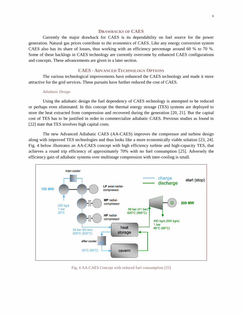
The new Advanced Adiabatic CAES (AA-CAES) improves the compressor and turbine design

along with improved TES technologies and thus looks like a more economically viable solution [23, 24].

Fig. 4 below illustrates an AA-CAES concept with high efficiency turbine and high-capacity TES, that

achieves a round trip efficiency of approximately 70% with no fuel consumption [25]. Adversely the

efficiency gain of adiabatic systems over multistage compression with inter-cooling is small.

Fig. 4 AA-CAES Concept with reduced fuel consumption [25]

7

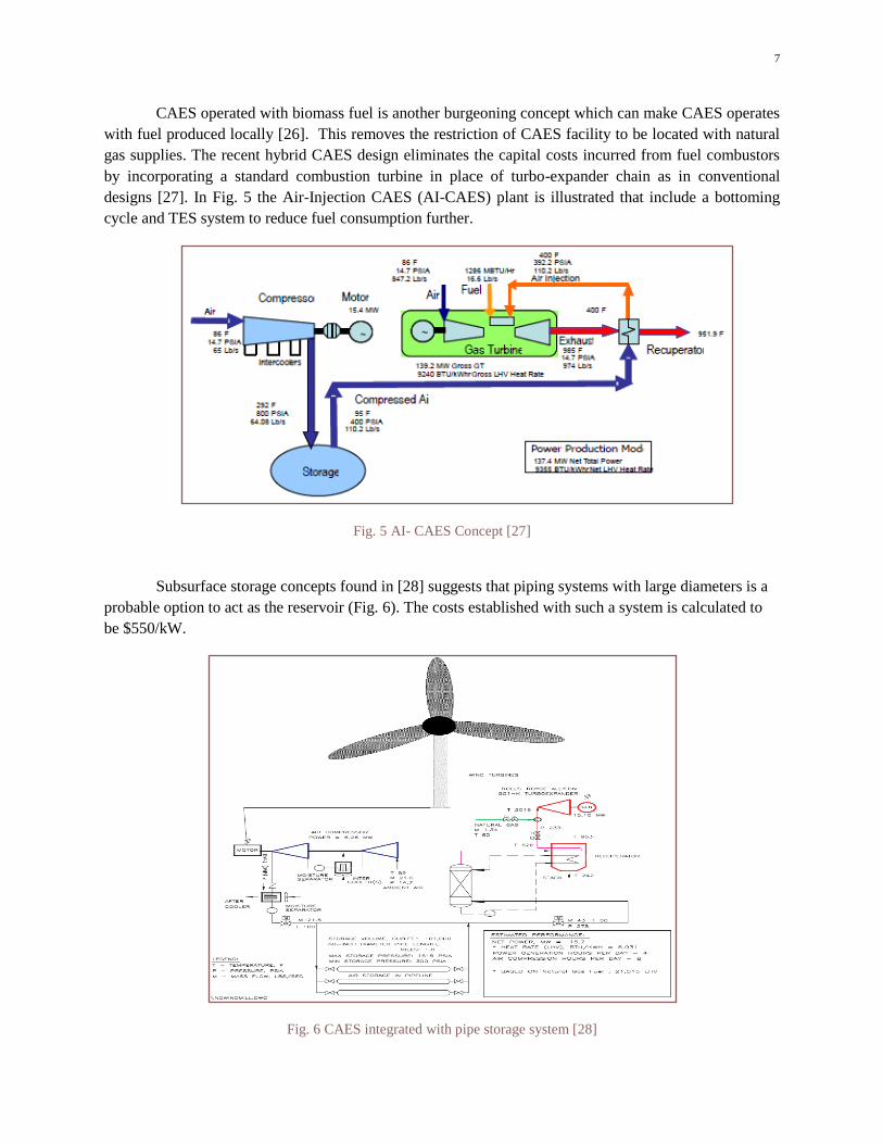
CAES operated with biomass fuel is another burgeoning concept which can make CAES operates

with fuel produced locally [26]. This removes the restriction of CAES facility to be located with natural

gas supplies. The recent hybrid CAES design eliminates the capital costs incurred from fuel combustors

by incorporating a standard combustion turbine in place of turbo-expander chain as in conventional

designs [27]. In Fig. 5 the Air-Injection CAES (AI-CAES) plant is illustrated that include a bottoming

cycle and TES system to reduce fuel consumption further.

Fig. 5 AI- CAES Concept [27]

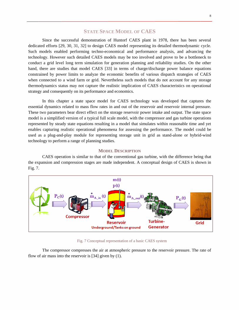
Subsurface storage concepts found in [28] suggests that piping systems with large diameters is a

probable option to act as the reservoir (Fig. 6). The costs established with such a system is calculated to

be $550/kW.

Fig. 6 CAES integrated with pipe storage system [28]

8

STATE SPACE MODEL OF CAES

Since the successful demonstration of Huntorf CAES plant in 1978, there has been several

dedicated efforts [29, 30, 31, 32] to design CAES model representing its detailed thermodynamic cycle.

Such models enabled performing techno-economical and performance analysis, and advancing the

technology. However such detailed CAES models may be too involved and prove to be a bottleneck to

conduct a grid level long term simulation for generation planning and reliability studies. On the other

hand, there are studies that model CAES [33] in terms of charge/discharge power balance equations

constrained by power limits to analyze the economic benefits of various dispatch strategies of CAES

when connected to a wind farm or grid. Nevertheless such models that do not account for any storage

thermodynamics status may not capture the realistic implication of CAES characteristics on operational

strategy and consequently on its performance and economics.

In this chapter a state space model for CAES technology was developed that captures the

essential dynamics related to mass flow rates in and out of the reservoir and reservoir internal pressure.

These two parameters bear direct effect on the storage reservoir power intake and output. The state space

model is a simplified version of a typical full scale model, with the compressor and gas turbine operations

represented by steady state equations resulting in a model that simulates within reasonable time and yet

enables capturing realistic operational phenomena for assessing the performance. The model could be

used as a plug-and-play module for representing storage unit in grid as stand-alone or hybrid-wind

technology to perform a range of planning studies.

MODEL DESCRIPTION

CAES operation is similar to that of the conventional gas turbine, with the difference being that

the expansion and compression stages are made independent. A conceptual design of CAES is shown in

Fig. 7.

Fig. 7 Conceptual representation of a basic CAES system

The compressor compresses the air at atmospheric pressure to the reservoir pressure. The rate of

flow of air mass into the reservoir is [34] given by (1).

9

1

1

1

21

.

_

P

PTc

Pm

inp

cinA

(1)

= Cp1/ Cv1 (2)

where cP is input power to the compressor (kW), Cp1 is the specific heat at constant pressure, 2P and

1P are the compressor output pressure and input pressure, respectively (in bar), Tin is ambient

temperature at input of Compressor (K), and Cv1 is specific heat at constant volume.

The turbine is modeled as a double stage air turbine. The compressed air from the reservoir is

compressed in a high pressure stage, and subsequently combusted with fuel in a low pressure stage. The

mass of air discharged from the reservoir is calculated using the turbine equation [35]. The rate of flow of

air discharged from the reservoir is given by (3).

1 1

1 1

.

_1 1.

_ 1 1 22 2 .

2 2 1 2

1 1 1

GA out

k k

k kA out p b

M G p

pFuel

Pm

c T PPmc T

c T P Pm

(3)

where, PG is the power (kW) delivered by gas turbine of CAES, T1 is the HP turbine inlet temperature

(K), T2 is the LP turbine inlet temperature (K), P1 and P2 are the pressures in LP and HP turbines (in

bar). Pb is the atmospheric pressure, . .

_A out Fuelm m is the ratio of the air discharge rate from the

reservoir to the rate of flow of fuel that combines in the combustion chamber to generate electricity, and

is the CAES round trip efficiency. We could also have charging and discharging efficiencies in equations

(1) and (3) respectively, instead of round trip efficiency of CAES [33].

The compressor and turbine ratings influence the charging and discharging times of the reservoir.

Depending upon the application, i.e., either to provide regulation service or as reserves, the charging and

discharging rates are determined. For instance, in the Huntorf the discharge/charge ratio is 1:2.Inside the

reservoir as the compressor pumps in air, the mass of air increases and simultaneously, the pressure of the

reservoir increases. Typically, the reservoir operates within the pressure range of 15 to 70 bar. The CAES

reservoir can be an underground storage, depleted natural gas/oil fields, piping systems or compressed air

tanks with different ratings. The mass and pressure inside the reservoir is computed by [36],

dtmdtmmoutAinA _

.

_

.

(4)

10

dtTmdtTm

V

Rp s

outAin

inA..

_

.

_

.

(5)

where R is the gas constant (J kg−1 K−1), V is the volume of the storage(m3), Tin is temperature at input

of storage and Ts is the temperature at which the compressed air is stored in the storage (K). This design

where the pressure changes with the mass of air is referred to as sliding pressure [36].

The state space representation of the model is,

_ _

_ _

( 1) ( ) ( )1 01 0

0 10 1 ( )( 1) ( )

A in A in CC

G GA out A out

m t m t P tK

K P tm t m t

(6)

_

_

1 1 ( )( 1)

( 1) ( )

A in

in SA out

m tm t

R RT TV Vp t m t

(7)

where KC and KG are the denominators of the equations (1) and (3) respectively. The energy that the

reservoir can store is determined by the pressure and mass values of the reservoir. In real time, the

reservoir cannot be discharged below a minimum pressure and charged beyond a maximum pressure

limit. This model facilitates enforcing this operational constraint during the simulation by conducting the

charging and discharging of CAES reservoir within the operational pressure ranges. The gradual pressure

leakage from the reservoir of 15bar/hour [37] is also accounted in this model. Thus the model facilitates

capturing the effect of internal storage dynamics on performance and economic indices. The power

compressed in and generated from the CAES obtained from simulation can be used in conjunction with

heat rate of turbine, hourly natural gas and spot prices to compute operational cost and revenue.

MODEL VALIDATION WITH HUNTORF OPERATIONAL DATA

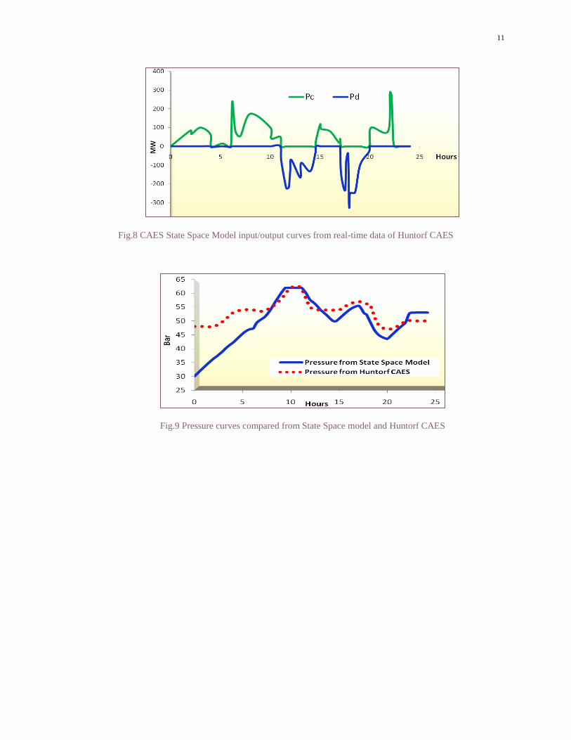
The CAES model was validated with the output curves from the Huntorf model [37]. The input

power Pc and output power Pd curves to the state space model are shown in Fig.8. These curves are the

real-time input/output power to the Huntorf CAES. The pressure from the state space model was

compared to the Huntorf CAES and verified its operation. As can be seen from Fig.9 that the Huntorf

CAES pressure ranges between 48 – 62 bars while the state space model pressure ranges from 30-62 bar.

The pressure for the state space model starts from 30 bar as the CAES reservoir was charged from empty

to full. On the otherhand the Huntorf model real time data is a snapshot from its real time operation and

had previously charged its reservoir with corresponding pressure of 48 bar.

11

Fig.8 CAES State Space Model input/output curves from real-time data of Huntorf CAES

Fig.9 Pressure curves compared from State Space model and Huntorf CAES

12

PERFORMANCE & ECONOMIC CHARACTERIZATION

A performance assessment of CAES using this model was presented in the PES General Meeting

paper [38]. The details of this study are given in the following section, where a number of performance

and economic indices that can be computed using a one year simulation of CAES plant are defined. These

can be used as criteria to evaluate the worth of different CAES configurations.

PERFORMANCE INDICES

Charging time:

Charging time, TCharge, is defined as the time taken to charge the storage reservoir to its full capacity

within the maximum pressure limit. It depends on the reservoir volume and compressor rating, and is

expressed in hours

Discharging time:

Discharging time, TDischarge, is defined as the time taken to discharge the storage reservoir from

its full capacity (at maximum pressure limit) to minimum pressure limit. It depends on the reservoir

volume and turbine rating, and is expressed in hours.

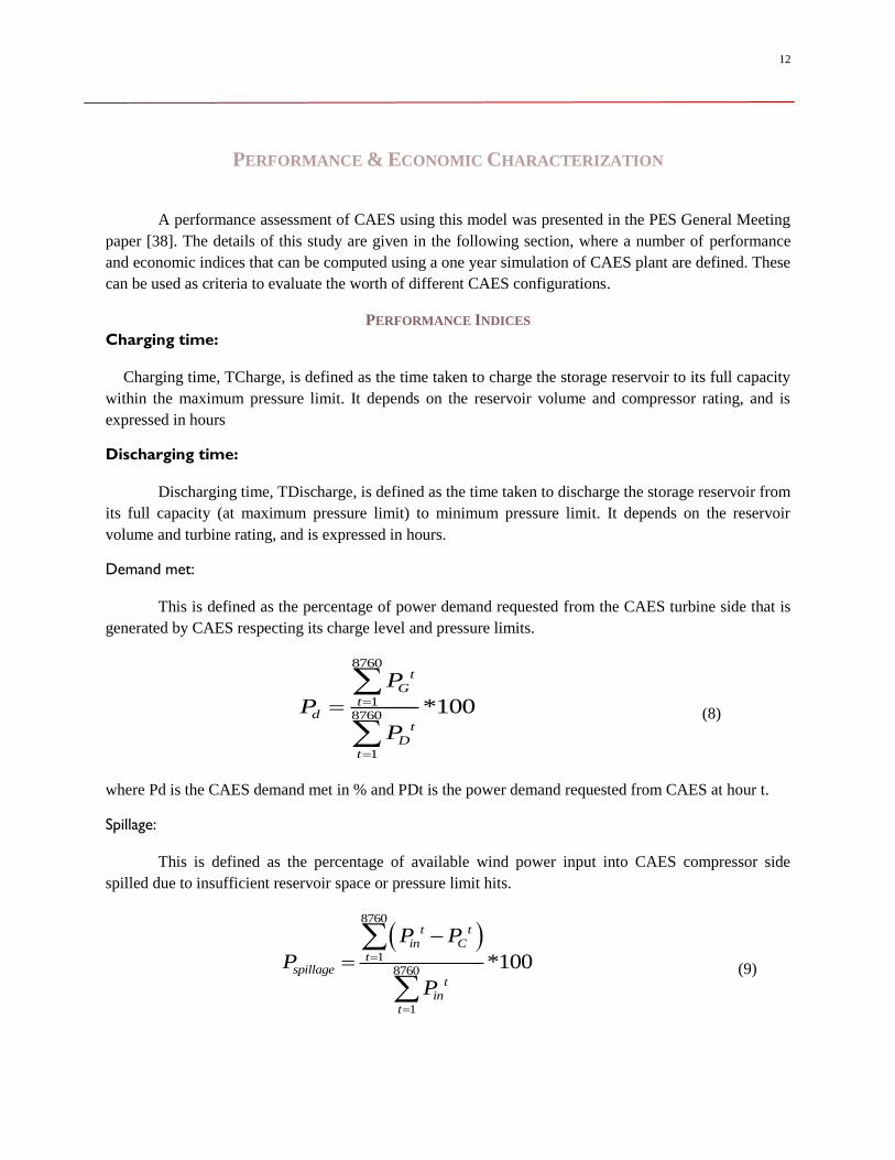
Demand met:

This is defined as the percentage of power demand requested from the CAES turbine side that is

generated by CAES respecting its charge level and pressure limits.

8760

18760

1

*100

t

Gt

dt

Dt

P

P

P

(8)

where Pd is the CAES demand met in % and PDt is the power demand requested from CAES at hour t.

Spillage:

This is defined as the percentage of available wind power input into CAES compressor side

spilled due to insufficient reservoir space or pressure limit hits.

8760

18760

1

*100

t t

in Ct

spillaget

int

P P

P

P

(9)

13

where Pspillage is the CAES input power spilled in %, Pint is the power input command into CAES at

hour t. Pct is the power compressed by the CAES compressor at hour t.

Carbon emissions:

Traditionally reserves are fossil fuel units, and in this case we assume them as coal units. When

the CAES facility is unable to meet the demand, it is supplied by such reserve units. Thus the cumulative

carbon emissions from the natural gas turbine of CAES and the coal unit are calculated. This index also

serves to quantify the advantages of CAES.

8760

1

( )t t t

NG G Coal D Gt

CE E P E P P

(10)

where CE is the carbon emissions from CAES and coal unit in tons/year, ENG and ECoal are the carbon

emissions from natural gas unit and from coal unit in tons/kWh.

ECONOMIC INDICES

According to the current market policies, some of the avenues that bear significant impact on

CAES economics and revenue would be energy arbitrage, charging cost, frequency regulation, spinning

reserves, installed capacity, market revenues (ICAP), system upgrade cost deferral, and environmental

impacts [39, 40]. For instance, revenue from energy arbitrage will be drawn by strategically charging and

discharging CAES in order to take advantage of the differences in peak-load and off-peak load prices.

This means that the decision on CAES configuration will also depend on the application. For higher

energy arbitrage, a CAES configuration with higher power density is suitable. In the case of revenue

opportunity from frequency regulation, there is a great potential if CAES responds appropriately to ISO

regulation signals. Then it stands a chance to be paid for both charging and discharging. Optimal

placement of CAES in the system could possibly defer transmission and distribution upgrade costs,

generating benefits of about 0.15- 1 M$/MW-year [41].

In this section, we have defined some traditional as well explorative economic indices, which can

be used to evaluate the economic value of CAES. Some of the indices are defined in relation to CAES

operating with a collocated wind farm.

CAES Cost:

Investment cost of CAES is the combination of investment costs required for turbine, compressor

and reservoir. The turbine rating translates into power rating of the CAES, and reservoir rating translates

into the energy rating of the CAES.

INV Tur T CR CC = P C P C Rated CE S (11)

argRated Tur Disch eE P T (12)

14

where CINV is the investment cost of CAES in $/kW, PTur is the turbine power rating in MW, PCR is

the compressor power rating in MW, CT is the turbine cost in $/kW, CC is the compressor cost in $/kW,

ERated is the energy rating of CAES in kWh, SC is the CAES storage capacity cost in $/kWh,

TDischarge is the discharge time of reservoir in hours.

Since TDischarge is a function of reservoir volume, it reflects the reservoir investment. For a

particular turbine rating and pressure limit, higher the reservoir capacity higher is the discharge time.

Operational cost of CAES:

CAES consumes natural gas in the process of generation of electricity. The cost associated with

fuel consumption and operation & maintenance over a year is calculated as operational cost per year.

8760

OP G NGt 1

C = HR P Ct t

Tur FOMP C

(13)

where COP is the operational cost in $/year, PG is the power generated by CAES in MW at hour t, HR is

the CAES heat rate in MBtu/MWh, CNG is the natural gas price in $/MBtu at hour t, and CFOM is the

annual fixed operation & maintenance cost of CAES in $/kW.

Operational revenue from CAES:

The hourly electricity prices (LMPs) over a year are used to compute the operational revenue.

8760

1

t t

R G ht

C P E

(14)

where CR is the operational revenue from CAES in $/year, Eh is the hourly electricity prices in $/kWh.

Production Tax Credit (PTC):

This is a business credit to the wind farm owner and is equivalent to the electricity generated

from the facility. This typically applies for the first 10 years of the wind plant operation. If the CAES

facility is collocated with the wind farm, then more electricity is generated by the wind facility with

CAES‘s support. This increases the tax credits.

8760

1

t

CAES G PTCt

PTC P T

(15)

where PTCCAES is the production tax credit through CAES in $, TPTC is the tax credit in $/kWh.

Revenue opportunity lost due to wind spillage:

We propose a new index to quantify the spillage defined above as an equivalent loss in revenue

opportunity, i.e., if there was an opportunity to store the spilled power and sell it at yearly average spot

price. This could be used to strike a comparison between many CAES configurations.

15

8760

1

( )t t

orl in ct

S EP P P

(16)

where Sorl is the spillage opportunity revenue loss in $/year, η is the round trip efficiency of CAES, EP is

the average electricity price $/kWh.

Credit from reserve saved:

Assuming the energy supplied by CAES to the system is typically obtained from reserves, in the

presence of CAES facility the reserve required by the system is reduced, which could contribute to the

yearly credits.

8760

1

t t

G pt

RC P R

(17)

where RC is the reserve credits due to CAES in $/year, Rp is the hourly reserve price in $/kWh.

Credits due to carbon tax reduced:

In the same manner as the carbon emissions, the carbon tax is calculated. With CAES, we can

expect reduction in this tax.

8760

1

( )t

G Coal NGt

CT P T T

(18)

where CT is the carbon tax credit due to CAES in $/year, TNG is the carbon tax for natural gas unit in

$/kWh, TCoal is the carbon tax for coal unit in $/kWh.

Payback Period for CAES:

It is defined as the number of years required to recover the invested amount on CAES facility

through revenues. It can be computed by solving the below cost balance equation,

0 0

1 1. . 10

(1 ) (1 )

N N

INV OP CAESn nn n

C C NR PTCr r

(19)

0

1 ( 10 )( )(1 )

N

INV CAESn

OPn

C PTCNR Cr

(20)

where n is the payback period, r is the rate of interest, and NR is the net revenue per year given by

RC RC CT .

If the CAES is not collocated with wind farm during the first 10 years of wind farm operation,

then the above equations will not include the PTCCAES term. So it is treated separately from the net

revenue per year term in the above equation.

16

NUMERICAL RESULTS

Study Description

This model can be run to simulate and analyze a stand-alone CAES or CAES collocated with

wind-farm scenario. To illustrate the functionality and features of this model the CAES facility was

designed to be co-located in a wind farm. This study would demonstrate how CAES mitigates the wind

variability, increases the capacity factor, benefits environment and also generates excess revenue

opportunities for the wind farm owners. This study is the forerunner for other storage technology

evaluation under a hybrid wind farm scenario to answer the pressing question is storage economically

viable for individual wind farm owners. In a sense we are investigating whether to mitigate the variability

of renewable at individual plant level or at the system level.

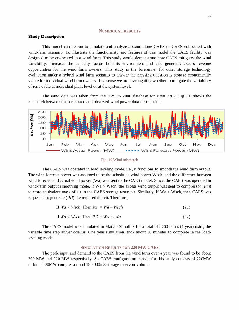
The wind data was taken from the EWITS 2006 database for site# 2302. Fig. 10 shows the

mismatch between the forecasted and observed wind power data for this site.

Fig. 10 Wind mismatch

The CAES was operated in load leveling mode, i.e., it functions to smooth the wind farm output.

The wind forecast power was assumed to be the scheduled wind power Wsch, and the difference between

wind forecast and actual wind power (Wa) was sent to the CAES model. Since, the CAES was operated in

wind-farm output smoothing mode, if Wa > Wsch, the excess wind output was sent to compressor (Pin)

to store equivalent mass of air in the CAES storage reservoir. Similarly, if Wa < Wsch, then CAES was

requested to generate (PD) the required deficit. Therefore,

If Wa > Wsch, Then Pin = Wa – Wsch (21)

If Wa < Wsch, Then PD = Wsch- Wa (22)

The CAES model was simulated in Matlab Simulink for a total of 8760 hours (1 year) using the

variable time step solver ode23s. One year simulation, took about 10 minutes to complete in the load-

leveling mode.

SIMULATION RESULTS FOR 220 MW CAES

The peak input and demand to the CAES from the wind farm over a year was found to be about

200 MW and 220 MW respectively. So CAES configuration chosen for this study consists of 220MW

turbine, 200MW compressor and 150,000m3 storage reservoir volume.

17

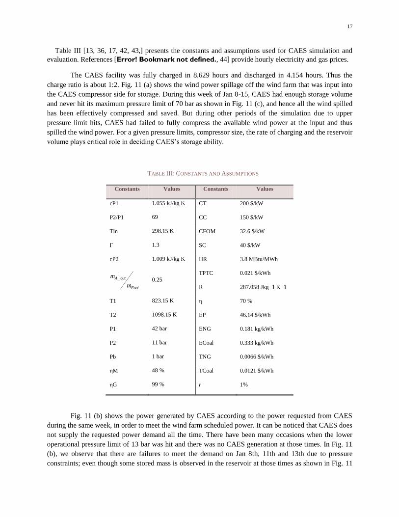
Table III [13, 36, 17, 42, 43,] presents the constants and assumptions used for CAES simulation and

evaluation. References [Error! Bookmark not defined., 44] provide hourly electricity and gas prices.

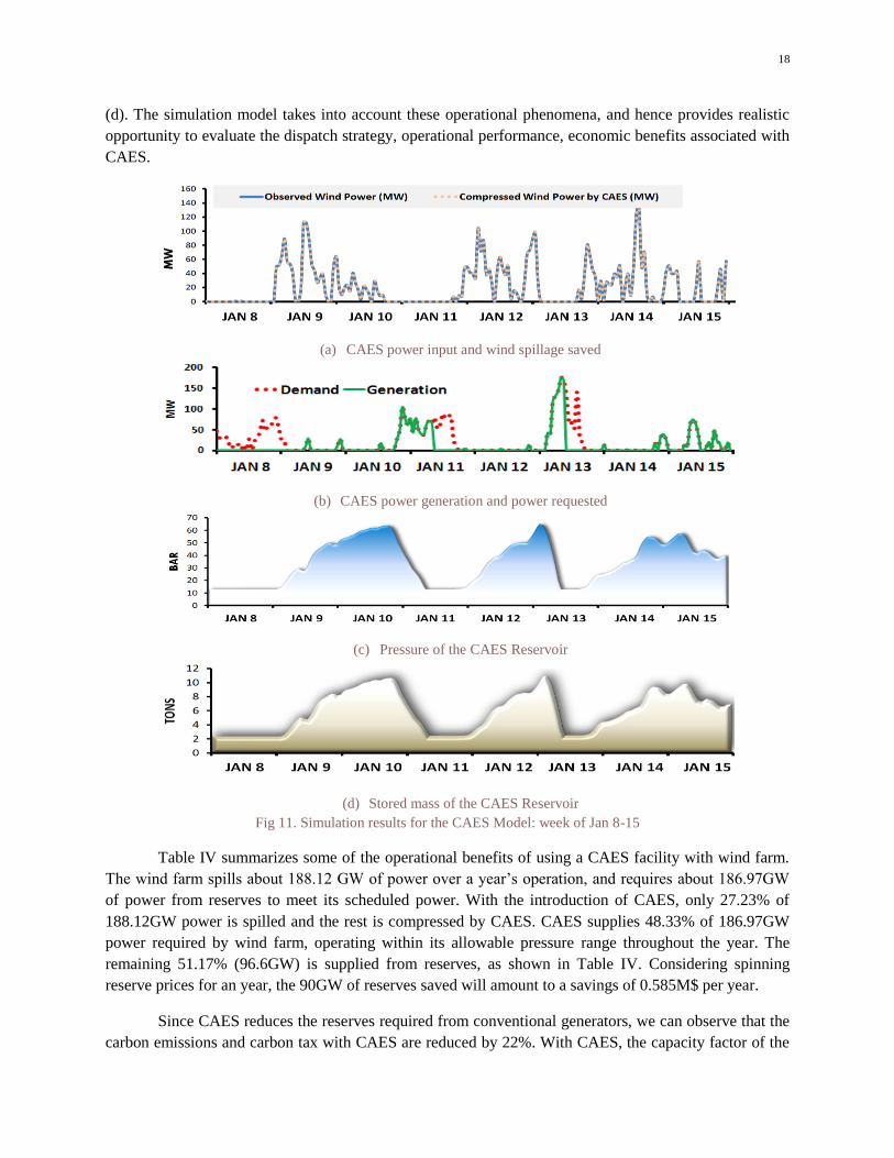
The CAES facility was fully charged in 8.629 hours and discharged in 4.154 hours. Thus the

charge ratio is about 1:2. Fig. 11 (a) shows the wind power spillage off the wind farm that was input into

the CAES compressor side for storage. During this week of Jan 8-15, CAES had enough storage volume

and never hit its maximum pressure limit of 70 bar as shown in Fig. 11 (c), and hence all the wind spilled

has been effectively compressed and saved. But during other periods of the simulation due to upper

pressure limit hits, CAES had failed to fully compress the available wind power at the input and thus

spilled the wind power. For a given pressure limits, compressor size, the rate of charging and the reservoir

volume plays critical role in deciding CAES‘s storage ability.

TABLE III: CONSTANTS AND ASSUMPTIONS

Constants Values Constants Values

cP1 1.055 kJ/kg K CT 200 $/kW

P2/P1 69 CC 150 $/kW

Tin 298.15 K CFOM 32.6 $/kW

Γ 1.3 SC 40 $/kW

cP2 1.009 kJ/kg K HR 3.8 MBtu/MWh

.

._A out

Fuel

m

m

0.25 TPTC 0.021 $/kWh

R 287.058 Jkg−1 K−1

T1 823.15 K η 70 %

T2 1098.15 K EP 46.14 $/kWh

P1 42 bar ENG 0.181 kg/kWh

P2 11 bar ECoal 0.333 kg/kWh

Pb 1 bar TNG 0.0066 $/kWh

ηM 48 % TCoal 0.0121 $/kWh

ηG 99 % r 1%

Fig. 11 (b) shows the power generated by CAES according to the power requested from CAES

during the same week, in order to meet the wind farm scheduled power. It can be noticed that CAES does

not supply the requested power demand all the time. There have been many occasions when the lower

operational pressure limit of 13 bar was hit and there was no CAES generation at those times. In Fig. 11

(b), we observe that there are failures to meet the demand on Jan 8th, 11th and 13th due to pressure

constraints; even though some stored mass is observed in the reservoir at those times as shown in Fig. 11

18

(d). The simulation model takes into account these operational phenomena, and hence provides realistic

opportunity to evaluate the dispatch strategy, operational performance, economic benefits associated with

CAES.

(a) CAES power input and wind spillage saved

(b) CAES power generation and power requested

(c) Pressure of the CAES Reservoir

(d) Stored mass of the CAES Reservoir

Fig 11. Simulation results for the CAES Model: week of Jan 8-15

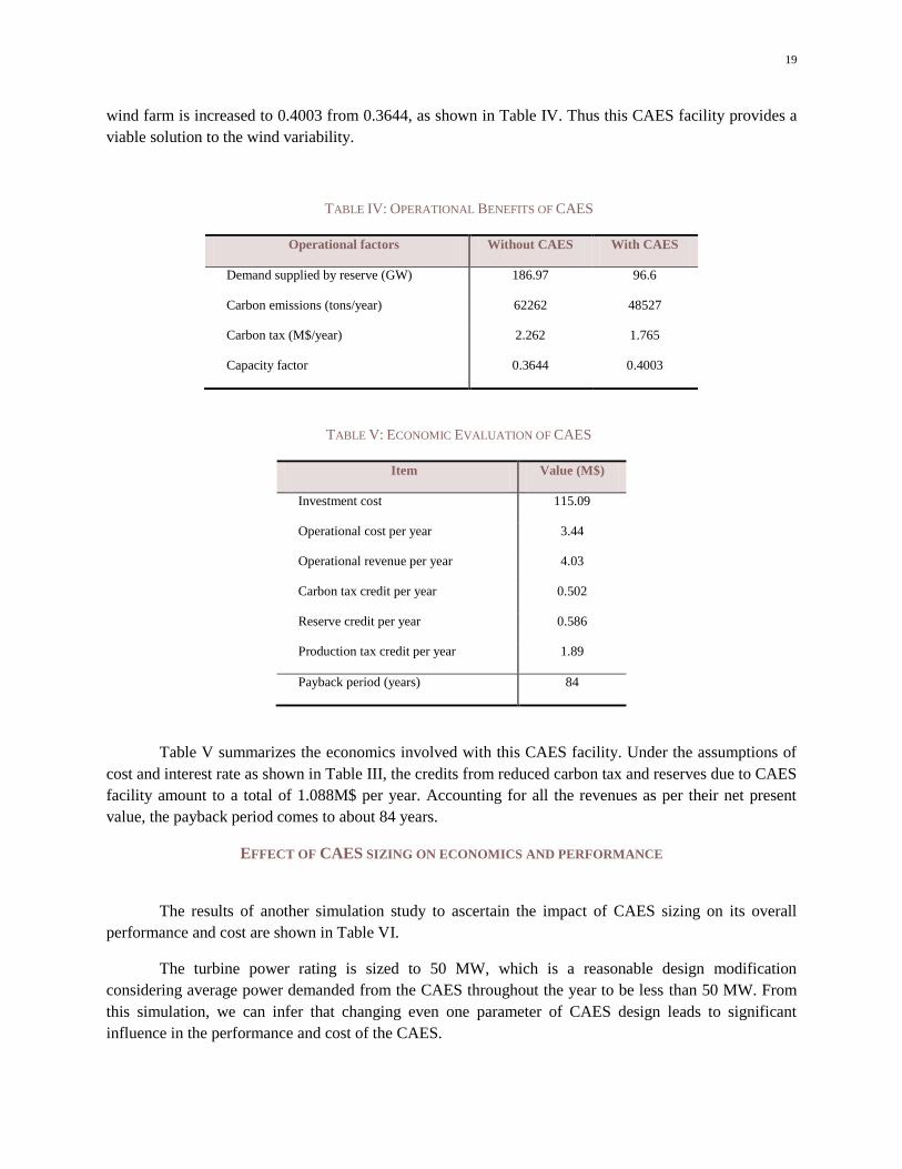
Table IV summarizes some of the operational benefits of using a CAES facility with wind farm.

The wind farm spills about 188.12 GW of power over a year‘s operation, and requires about 186.97GW

of power from reserves to meet its scheduled power. With the introduction of CAES, only 27.23% of

188.12GW power is spilled and the rest is compressed by CAES. CAES supplies 48.33% of 186.97GW

power required by wind farm, operating within its allowable pressure range throughout the year. The

remaining 51.17% (96.6GW) is supplied from reserves, as shown in Table IV. Considering spinning

reserve prices for an year, the 90GW of reserves saved will amount to a savings of 0.585M$ per year.

Since CAES reduces the reserves required from conventional generators, we can observe that the

carbon emissions and carbon tax with CAES are reduced by 22%. With CAES, the capacity factor of the

19

wind farm is increased to 0.4003 from 0.3644, as shown in Table IV. Thus this CAES facility provides a

viable solution to the wind variability.

TABLE IV: OPERATIONAL BENEFITS OF CAES

Operational factors Without CAES With CAES

Demand supplied by reserve (GW) 186.97 96.6

Carbon emissions (tons/year) 62262 48527

Carbon tax (M$/year) 2.262 1.765

Capacity factor 0.3644 0.4003

TABLE V: ECONOMIC EVALUATION OF CAES

Item Value (M$)

Investment cost 115.09

Operational cost per year 3.44

Operational revenue per year 4.03

Carbon tax credit per year 0.502

Reserve credit per year 0.586

Production tax credit per year 1.89

Payback period (years) 84

Table V summarizes the economics involved with this CAES facility. Under the assumptions of

cost and interest rate as shown in Table III, the credits from reduced carbon tax and reserves due to CAES

facility amount to a total of 1.088M$ per year. Accounting for all the revenues as per their net present

value, the payback period comes to about 84 years.

EFFECT OF CAES SIZING ON ECONOMICS AND PERFORMANCE

The results of another simulation study to ascertain the impact of CAES sizing on its overall

performance and cost are shown in Table VI.

The turbine power rating is sized to 50 MW, which is a reasonable design modification

considering average power demanded from the CAES throughout the year to be less than 50 MW. From

this simulation, we can infer that changing even one parameter of CAES design leads to significant

influence in the performance and cost of the CAES.

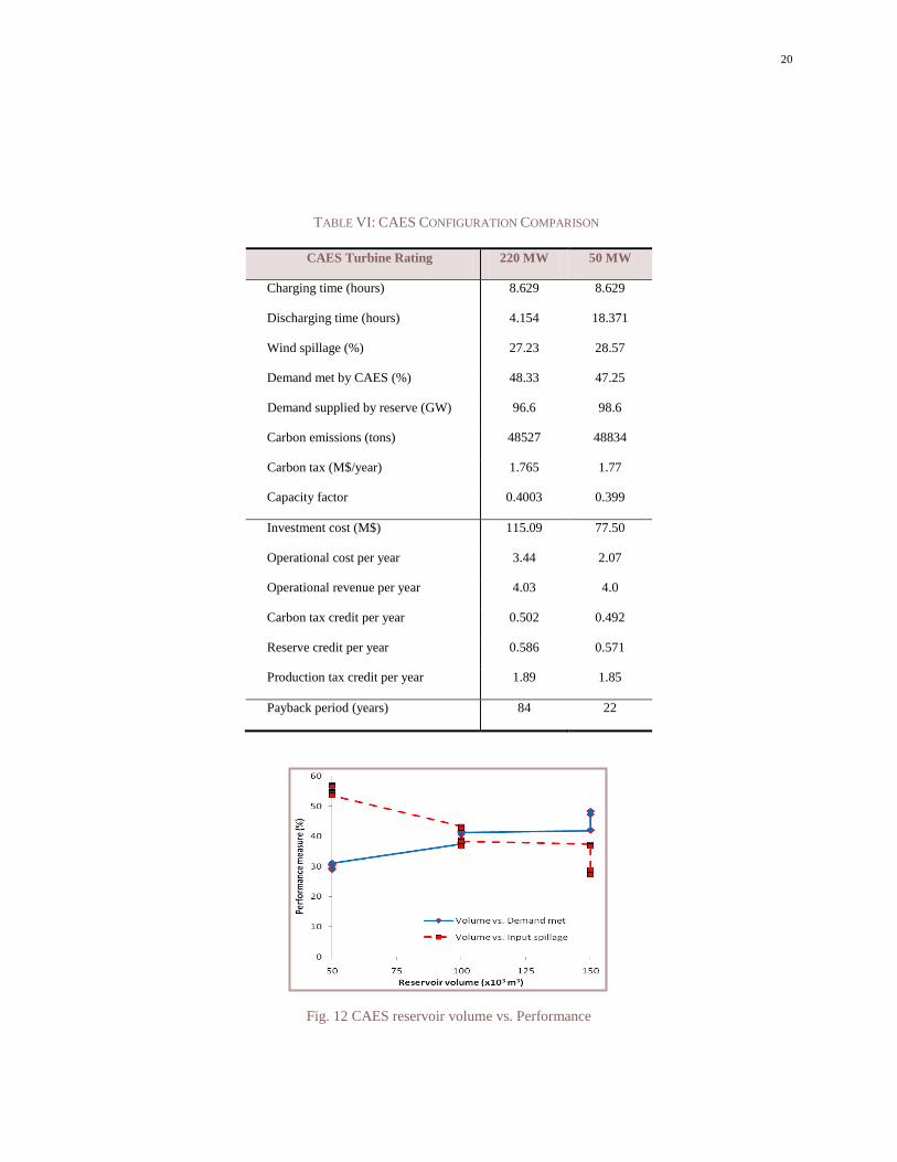
20

TABLE VI: CAES CONFIGURATION COMPARISON

CAES Turbine Rating 220 MW 50 MW

Charging time (hours) 8.629 8.629

Discharging time (hours) 4.154 18.371

Wind spillage (%) 27.23 28.57

Demand met by CAES (%) 48.33 47.25

Demand supplied by reserve (GW) 96.6 98.6

Carbon emissions (tons) 48527 48834

Carbon tax (M$/year) 1.765 1.77

Capacity factor 0.4003 0.399

Investment cost (M$) 115.09 77.50

Operational cost per year 3.44 2.07

Operational revenue per year 4.03 4.0

Carbon tax credit per year 0.502 0.492

Reserve credit per year 0.586 0.571

Production tax credit per year 1.89 1.85

Payback period (years) 84 22

Fig. 12 CAES reservoir volume vs. Performance

21

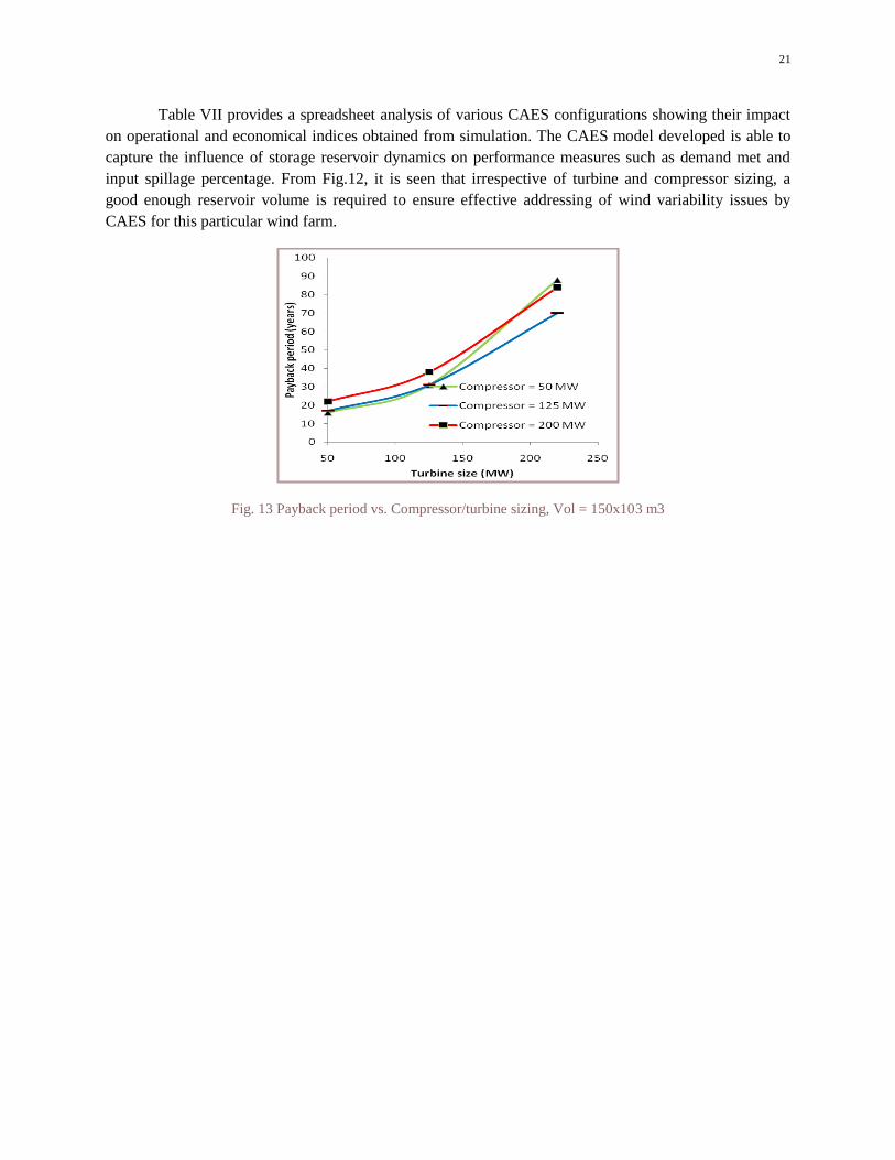
Table VII provides a spreadsheet analysis of various CAES configurations showing their impact

on operational and economical indices obtained from simulation. The CAES model developed is able to

capture the influence of storage reservoir dynamics on performance measures such as demand met and

input spillage percentage. From Fig.12, it is seen that irrespective of turbine and compressor sizing, a

good enough reservoir volume is required to ensure effective addressing of wind variability issues by

CAES for this particular wind farm.

Fig. 13 Payback period vs. Compressor/turbine sizing, Vol = 150x103 m3

22

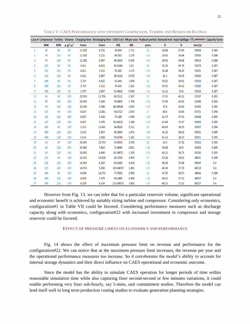
TABLE V: CAES PERFORMANCE WITH DIFFERENT COMPRESSOR, TURBINE AND RESERVOIR RATINGS

However from Fig. 13, we can infer that for a particular reservoir volume, significant operational

and economic benefit is achieved by suitably sizing turbine and compressor. Considering only economics,

configuration#1 in Table VII could be favored. Considering performance measures such as discharge

capacity along with economics, configuration#22 with increased investment in compressor and storage

reservoir could be favored.

EFFECT OF PRESSURE LIMITS ON ECONOMICS AND PERFORMANCE

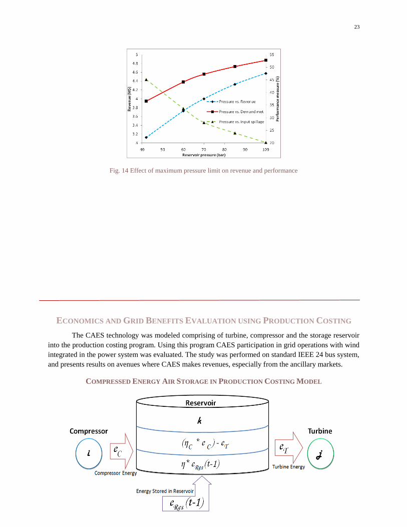
Fig. 14 shows the effect of maximum pressure limit on revenue and performance for the

configuration#22. We can notice that as the maximum pressure limit increases, the revenue per year and

the operational performance measures too increase. So it corroborates the model‘s ability to account for

internal storage dynamics and their direct influence on CAES operational and economic outcome.

Since the model has the ability to simulate CAES operation for longer periods of time within

reasonable simulation time while also capturing finer second-second or few minutes variations, it could

enable performing very finer sub-hourly, say 5-mins, unit commitment studies. Therefore the model can

lend itself well in long term production costing studies to evaluate generation planning strategies.

23

Fig. 14 Effect of maximum pressure limit on revenue and performance

ECONOMICS AND GRID BENEFITS EVALUATION USING PRODUCTION COSTING

The CAES technology was modeled comprising of turbine, compressor and the storage reservoir

into the production costing program. Using this program CAES participation in grid operations with wind

integrated in the power system was evaluated. The study was performed on standard IEEE 24 bus system,

and presents results on avenues where CAES makes revenues, especially from the ancillary markets.

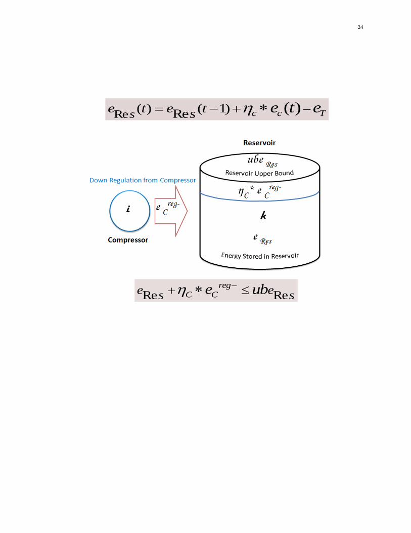
COMPRESSED ENERGY AIR STORAGE IN PRODUCTION COSTING MODEL

24

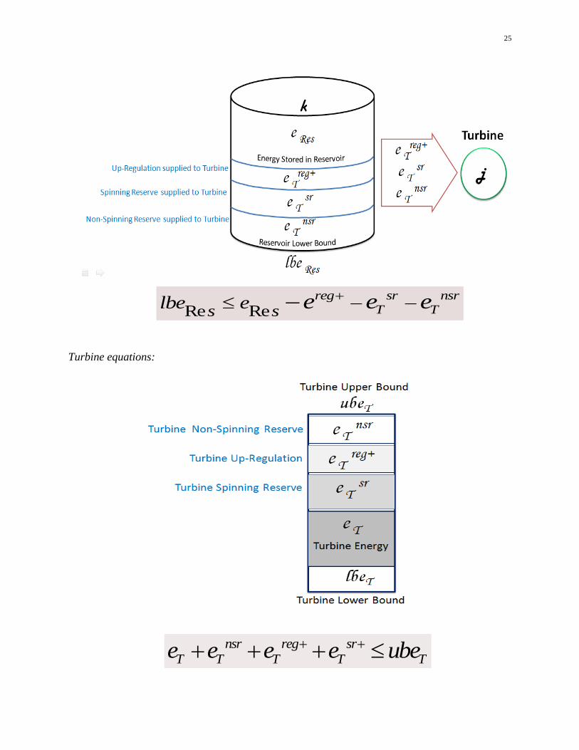
Re( ) ( 1)Re ( )c c Ts

e t e ts e t e

Re Rereg

C Ce es se ub

25

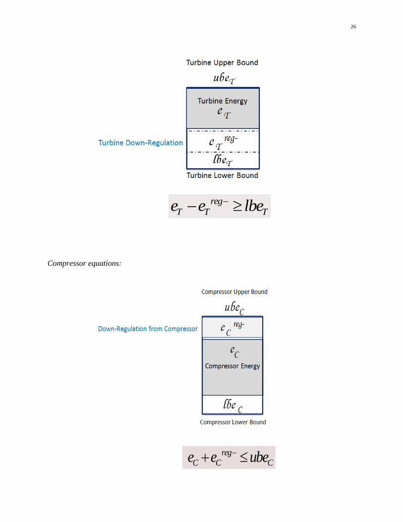
Turbine equations:

Re Rereg sr nsr

T Ts slbe e e e e

nsr reg sr

T T T T Te e e e ube

26

Compressor equations:

reg

T T Te e lbe

reg

C C Ce e ube

27

UNIT COMMITMENT PROBLEM FORMULATION

Minimize the sum of total energy and ancillary service costs for given biddings, the startup and shutdown

costs and loss of load penalties.

Subject to

Constraint 1: Scheduled generation meets scheduled demand (Kirchhoff‘s current law at every node)

Constraint 2: Generator minimum and maximum capacity limits

Constraint 3: DC-OPF transmission network formulation, with transmission line flow limits

Constraint 4: Energy + spinning reserves + up-regulation ≤ generator‘s maximum capacity

Constraint 5: Energy – down-regulation ≥ generator‘s minimum capacity

Constraint 6: Total spinning reserve requirement

Constraint 7: Total regulation (up and down) requirement

Constraint 8: Ramp up and down constraints

Constraint 9: Spinning reserve from generator i is limited by 10 times its ramping rate in MW/min

Constraint 10: Regulation from generator i is limited by its ramping rate in MW/min

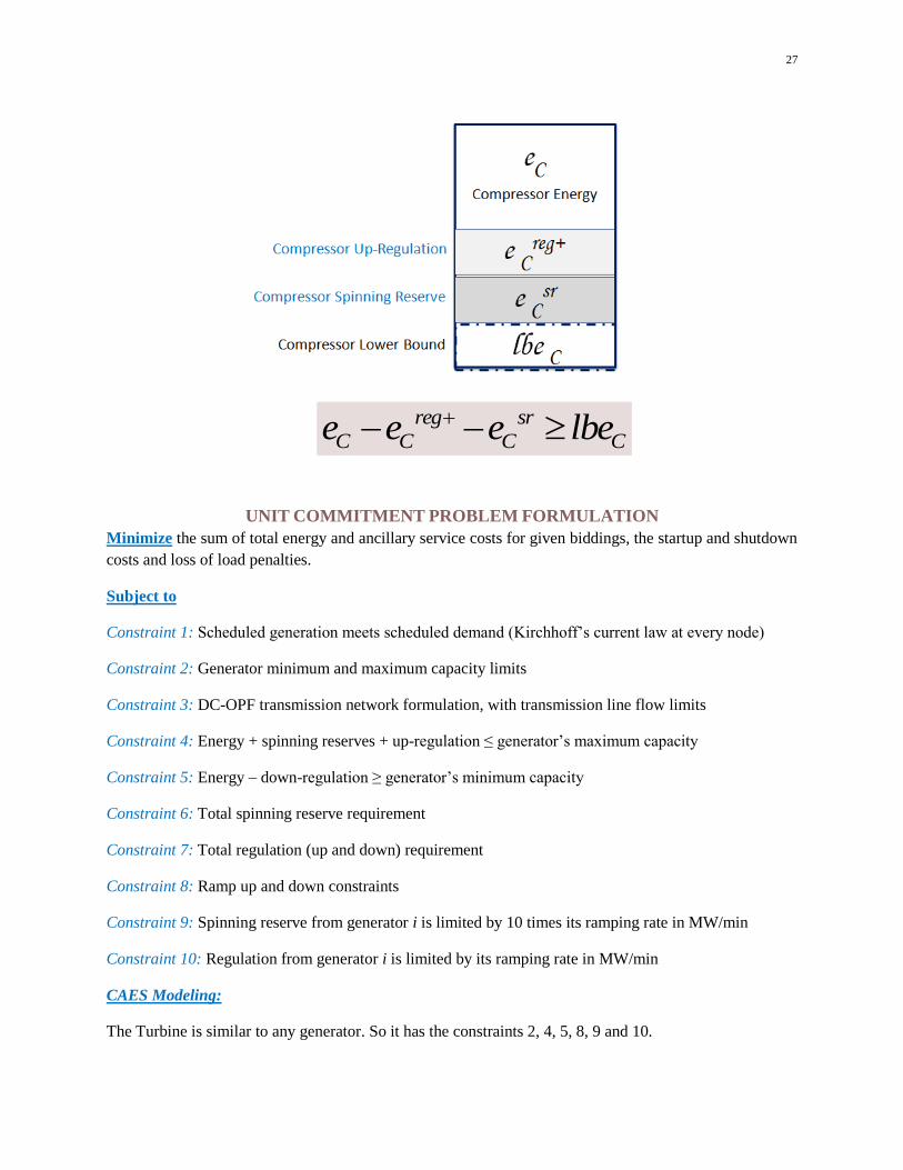
CAES Modeling:

The Turbine is similar to any generator. So it has the constraints 2, 4, 5, 8, 9 and 10.

reg sr

C C C Ce e e lbe

28

Compressor modeling:

Constraint 11: Energy + down-regulation ≤ compressor‘s maximum capacity

Constraint 12: Energy – spinning reserve – up-regulation ≥ compressor‘s minimum capacity

Storage reservoir modeling:

Constraint 13: Energy stored (t) = Energy stored (t-1) + η*Energycompr (t) – Energyturb (t)

Constraint 14: Energy stored + down-regulationcompr ≤ reservoir‘s maximum capacity

Constraint 15: Energy stored – spinning reserveturb – up-regulationturb ≥ reservoir‘s minimum capacity

ECONOMIC DISPATCH PROBLEM FORMULATION

The ED problem is similar with the UC problem in most parts except that uij is a parameter, not a

variable. Based on the commitment schedule (i.e., values of uij‗s) generated by the UC problem, the ED

problem dispatches the generating units and obtains Locational Marginal Prices (LMP) at each node for

energy and Market Clearing Prices (MCP) for ancillary service.

CASE STUDY

In IEEE 24-bus Reliability Test System (RTS) wind and CAES were integrated and production

costing studies were conducted. The production costing study is an hourly simulation for 48 hours (2

days). The data for load and wind generation is taken from Bonneville Power Administration (BPA) for

Nov 2nd and 3rd in the year 2010. This data was chosen as it covered good variation in wind pattern. The

program was developed using MATLAB with TOMLAB optimization platform.

ANCILLARY SERVICE REQUIREMENTS

Ever since the advent of the power system operations, the system is forced to run with sub-

optimal mix of generation due to the forecast errors in load and generation offers, as well as the

unforeseen errors. The integration of renewable, especially wind has further worsened the situation due to

its highly variable nature. Hence power generation and load is balanced over several time frames. The

generation offers are dispatched to match the actual loads in the real time. The uncontrolled generation

and actual load fluctuations are categorized as load following and regulation. Regulation is a capacity

service dedicated to compensate for the unscheduled minute-to-minute fluctuations in the system loads

and generation [45]. This does not involve any net energy. While load following are largely correlated

deviation of system load and generation from its predicted pattern within the time scale of ten minutes

with slow ramps and fewer sign changes. The intra-hour 10-minutes variations are addressed by

deploying necessary spinning reserves in this simulation. The hourly operating reserve is estimated as the

MW loss of generation due to the outage of the largest generating unit at each hour, 50% of which is

allocated for spinning reserves.

Some of the current practices for estimating regulation requirement are briefly presented in this

section. PJM regulation market [45] and Xcel Energy [46] use the regulation allocation method developed

29

by Oak Ridge National Laboratory (ORNL), which computes the regulation requirement from the

standard deviations of total system load and wind resources, assuming they are uncorrelated. ERCOT

finds the 98.8 percentile of net load changes and hourly regulation deployed over the past 30 days and

previous year net load changes, and considers the largest of these as the required regulation. Depending

upon the historical CPS-I score, it allocates extra 10% regulation at certain times [47]. CAISO calculates

its regulation requirement based on the intertie schedule changes, self-scheduled generation and actual

system demand variations over 20 minute intervals. CAISO calculates regulation up and down separately

based on the projected worst 10-minutes up and down ramps [48]. All these methods have one thing in

common, i.e., learning from the historical data of either net load changes or regulation allocated.

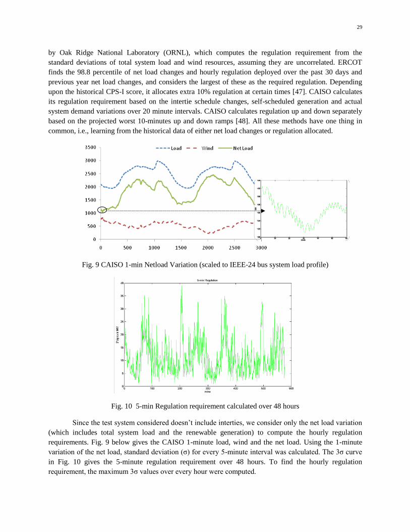
Fig. 9 CAISO 1-min Netload Variation (scaled to IEEE-24 bus system load profile)

Fig. 10 5-min Regulation requirement calculated over 48 hours

Since the test system considered doesn‘t include interties, we consider only the net load variation

(which includes total system load and the renewable generation) to compute the hourly regulation

requirements. Fig. 9 below gives the CAISO 1-minute load, wind and the net load. Using the 1-minute

variation of the net load, standard deviation (σ) for every 5-minute interval was calculated. The 3σ curve

in Fig. 10 gives the 5-minute regulation requirement over 48 hours. To find the hourly regulation

requirement, the maximum 3σ values over every hour were computed.

30

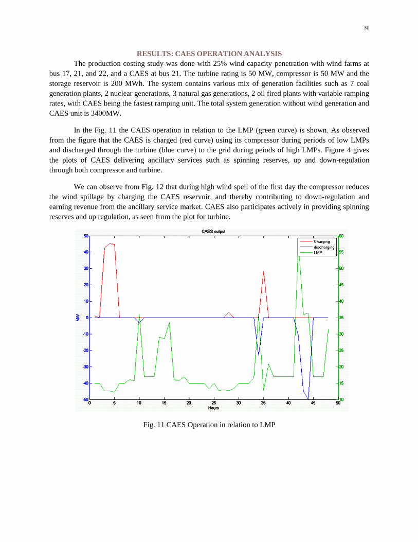
RESULTS: CAES OPERATION ANALYSIS

The production costing study was done with 25% wind capacity penetration with wind farms at

bus 17, 21, and 22, and a CAES at bus 21. The turbine rating is 50 MW, compressor is 50 MW and the

storage reservoir is 200 MWh. The system contains various mix of generation facilities such as 7 coal

generation plants, 2 nuclear generations, 3 natural gas generations, 2 oil fired plants with variable ramping

rates, with CAES being the fastest ramping unit. The total system generation without wind generation and

CAES unit is 3400MW.

In the Fig. 11 the CAES operation in relation to the LMP (green curve) is shown. As observed

from the figure that the CAES is charged (red curve) using its compressor during periods of low LMPs

and discharged through the turbine (blue curve) to the grid during peiods of high LMPs. Figure 4 gives

the plots of CAES delivering ancillary services such as spinning reserves, up and down-regulation

through both compressor and turbine.

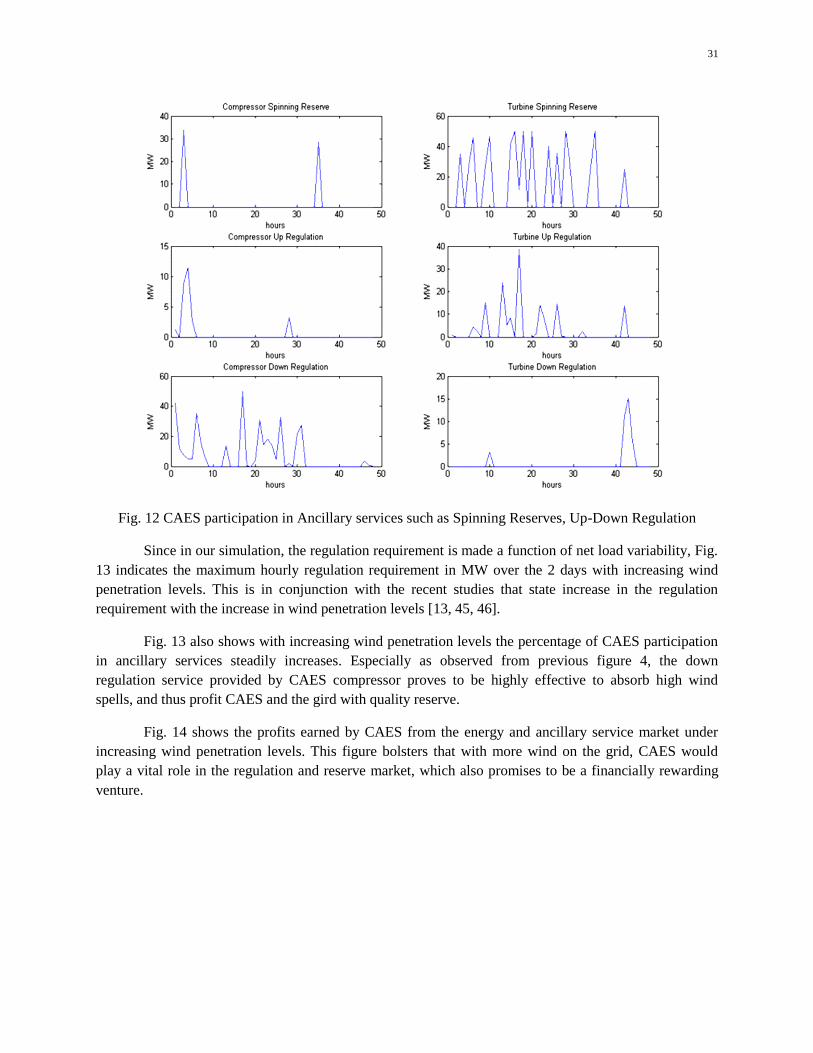
We can observe from Fig. 12 that during high wind spell of the first day the compressor reduces

the wind spillage by charging the CAES reservoir, and thereby contributing to down-regulation and

earning revenue from the ancillary service market. CAES also participates actively in providing spinning

reserves and up regulation, as seen from the plot for turbine.

Fig. 11 CAES Operation in relation to LMP

31

Fig. 12 CAES participation in Ancillary services such as Spinning Reserves, Up-Down Regulation

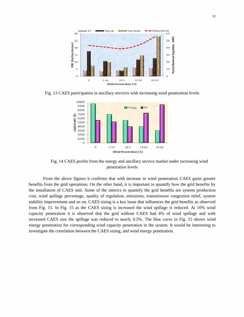
Since in our simulation, the regulation requirement is made a function of net load variability, Fig.

13 indicates the maximum hourly regulation requirement in MW over the 2 days with increasing wind

penetration levels. This is in conjunction with the recent studies that state increase in the regulation

requirement with the increase in wind penetration levels [13, 45, 46].

Fig. 13 also shows with increasing wind penetration levels the percentage of CAES participation

in ancillary services steadily increases. Especially as observed from previous figure 4, the down

regulation service provided by CAES compressor proves to be highly effective to absorb high wind

spells, and thus profit CAES and the gird with quality reserve.

Fig. 14 shows the profits earned by CAES from the energy and ancillary service market under

increasing wind penetration levels. This figure bolsters that with more wind on the grid, CAES would

play a vital role in the regulation and reserve market, which also promises to be a financially rewarding

venture.

32

Fig. 13 CAES participation in ancillary services with increasing wind penetration levels

Fig. 14 CAES profits from the energy and ancillary service market under increasing wind

penetration levels

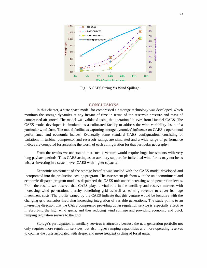
From the above figures it confirms that with increase in wind penetration CAES gains greater

benefits from the grid operations. On the other hand, it is important to quantify how the grid benefits by

the installation of CAES unit. Some of the metrics to quantify the grid benefits are system production

cost, wind spillage percentage, quality of regulation, emissions, transmission congestion relief, system

stability improvement and so on. CAES sizing is a key issue that influences the grid benefits as observed

from Fig. 15. In Fig. 15 as the CAES sizing is increased the wind spillage is reduced. At 10% wind

capacity penetration it is observed that the grid without CAES had 4% of wind spillage and with

increased CAES size the spillage was reduced to nearly 0.5%. The blue curve in Fig. 15 shows wind

energy penetration for corresponding wind capacity penetration in the system. It would be interesting to

investigate the correlation between the CAES sizing, and wind energy penetration.

33

Fig. 15 CAES Sizing Vs Wind Spillage

CONCLUSIONS

In this chapter, a state space model for compressed air storage technology was developed, which

monitors the storage dynamics at any instant of time in terms of the reservoir pressure and mass of

compressed air stored. The model was validated using the operational curves from Huntorf CAES. The

CAES model developed is simulated as a collocated facility to address the wind variability issue of a

particular wind farm. The model facilitates capturing storage dynamics‘ influence on CAES‘s operational

performance and economic indices. Eventually some standard CAES configurations consisting of

variations in turbine, compressor and reservoir ratings are simulated and a wide range of performance

indices are computed for assessing the worth of each configuration for that particular geography.

From the results we understand that such a venture would require huge investments with very

long payback periods. Thus CAES acting as an auxiliary support for individual wind farms may not be as

wise as investing in a system level CAES with higher capacity.

Economic assessment of the storage benefits was studied with the CAES model developed and

incorporated into the production costing program. The assessment platform with the unit commitment and

economic dispatch program modules dispatched the CAES unit under increasing wind penetration levels.

From the results we observe that CAES plays a vital role in the ancillary and reserve markets with

increasing wind penetration, thereby benefitting grid as well as earning revenue to cover its huge

investment costs. The profits earned by the CAES indicate that this venture would be lucrative with the

changing grid scenarios involving increasing integration of variable generations. The study points to an

interesting direction that the CAES compressor providing down regulation service is especially effective

in absorbing the high wind spells, and thus reducing wind spillage and providing economic and quick

ramping regulation service to the grid.

Storage‘s participation in ancillary services is attractive because the new generation portfolio not

only requires more regulation services, but also higher ramping capabilities and more operating reserves

to counter the costs associated with deeper and more frequent cycling of fossil units.

34

BIBLIOGRAPHY

[1] Bottling Electricity: Storage as a Strategic Tool for Managing Variability and Capacity Concerns in the Modern

Grid, The Electricity Advisory Committee, Dec 2008 - http://www.oe.energy.gov/eac.htm

[2]J.R. Sears, ―Thermal and Compressed Air Energy Storage (TACAS)‖, 2005

[3] Y.V. Makarov, et.al. ―Wide-Area Energy Storage and Management System to Balance Intermittent Resources in

the Booneville Power Administration and California ISO Control Areas‖ PNNL Report, 2008

[4] Schoenung. S.M, ―Characteristics and Technologies for Long-vs. Short-Term Energy Storage‖, A Study by the

DOE Energy Storage Systems Program, SAND2001-0765 2001

[5] Pier Final Project Report, ―An Assessment Of Battery And Hydrogen Energy Storage Systems Integrated With

Wind Energy Resources In California‖, University of California, Berkeley, September 2005

[6] Market.T, et.al, ― Energy Storage System Requirements for Hybrid Fuel Cell Vehicles‖, NREL Report, June

2003

[7] Bents.D.J and Scullin.V.J, ―Hydrogen-Oxygen PEM Regenerative Fuel Cell Energy Storage System‖ Glenn

Research Center, Jan 2005 Available Online: http://gltrs.grc.nasa.gov

[8] Energy Efficiency Factsheet – Washington State University, 2003 Online:

http://www.energy.wsu.edu/documents/engineering/Thermal.pdf

[9] Tabors Caramanis & Associates, ―Source Energy And Environmental Impacts Of Thermal Energy Storage‖,

California Energy Commission, 1996.

[10] Ise, T.; Kita, M.; Taguchi, A.;‖ A hybrid energy storage with a SMES and secondary battery‖, Applied

Superconductivity, IEEE Transactions on Volume 15, Issue 2, Part 2, June 2005 pp:1915 - 1918

[11] Huang.W, et.al., ―Discussion on application of super capacitor energy storage system in microgrid‖, Sustainable

Power Generation and Supply, 2009. SUPERGEN '09. International Conference on 6-7 April 2009 pp.1-4

[12] Ibrahim H, Ilinca A, Peroon J., ―Energy storage systems—Characteristics and comparisons‖ Science Direct, Jan

2007

[13] EPRI-DOE Handbook of Energy Storage for Transmission and Distribution Applications, 2003

[14] IET JOURNAL ― FULL CHARGE AHEAD‖

[15]E. Spahi, G. Balzer, B. Hellmich and W. Münch , ―Wind Energy Storages - Possibilities‖, PowerTech 2007.

Available Online: http://ieeexplore.ieee.org/stamp/stamp.jsp?tp=&arnumber=4538387&isnumber=4538278

[16] Ibrahim H, Ilinca A, Peroon J., ―Energy storage systems—Characteristics and comparisons‖ Science Direct, Jan

2007

[17]Brown Boveri, ―Huntorf Air Storage Gas Turbine Power Plant‖

[18] Succar, S. and R. Williams. ―Compressed Air Energy Storage: Theory, Operation, and Applications.‖ March

2008

[19] B.Haug, ―The Iowa Stored Energy Park – A Project Review and Update‖, May 2005

[20] B.Richard, ―Energy Storage – A Non Technical Guide ―, Pennwell Publication

[21] E. Macchi and G. Lozza, "Study Of Thermodynamic Performance Of Caes Plants,

Including Unsteady Effects," in Gas Turbine Conference and Exhibition,

Anaheim, CA, USA, 1987, p. 10.

[22]J.R. Sears, ―Thermal and Compressed Air Energy Storage (TACAS)‖, TACAS White Paper 2005. Online:

http://www.7x24exchange.org/lakemichigan/downloads/TACASWhitePaper.pdf

[23] G. Salgi and H. Lund, "Compressed air energy storage in Denmark : a feasibility

study and an overall energy system analysis," in World renewable energy congress IX Florence, Italy, 2006.

[24] C. Bullough, C. Gatzen, C. Jakiel, M. Koller, A. Nowi, and S. Zunft, "Advanced Adiabatic Compressed Air

Energy Storage for the Integration of Wind Energy," in European Wind Energy Conference London, UK: EWEA,

2004.

[25] B. Calaminus, "Innovative Adiabatic Compressed Air Energy Storage System of EnBW in Lower Saxony," in

2nd International Renewable Energy Storage conference (IRES II) Bonn, Germany, 2007.

[26] P. Denholm, ―Improving the technical, environmental and social performance of wind energy systems using

biomass-based energy storage,‖ National Renewable Energy Laboratory, 1617 Cole Boulevard, Golden, CO 80401-

3393, USA

[27] M. Nakhamkin, "Novel Compressed Air Energy Storage Concepts," in Electricity Storage Association Meeting

2006: Energy Storage in Action Knoxville, Tenn.: Energy Storage Association, 2006.

35

[28] Nakhamkin M, Wolk R, van der Linden S, Hall R, Bradshaw D. New compressed air energy storage concept

can improve the profitability of existing simple cycle, combined cycle, wind energy, and landfill gas combustion

turbine-based power plants. EESAT 2003 Conference San Francisco, CA, October 27–29, 2003.

[29] E. Macchi and G. Lozza, "Study Of Thermodynamic Performance Of Caes Plants, Including Unsteady Effects,"

Gas Turbine Conference and Exhibition, Anaheim, CA, USA, 1987, p. 10.

[30] P. Vadasz, and D. Weiner, ―Correlating Compressor and Turbine Costs to Thermodynamic Properties for

CAES Plants,‖ Cost Engineering, Vol. 29, No. 11, pp. 10-15, November 1987

[31] Nakhamkin, M., Swensen, E.C., Abitante, P.A.,Whims, M., Weiner, D., Vadasz, P., Brokman,S., ―Conceptual

Engineering of a 300 MW CAES Plant, Part 1: Cost Effectiveness Analysis,‖ 36th ASME International Gas Turbine

and Aeroengine Congress and Exposition, Fl., June 1991

[32]Vadasz, P, ―Compressed Air Energy Storage:Optimal Performance and Techno-Economical Indices‖, Int.J.

Applied Thermodynamics, Vol.2, 1999

[33] M.Korpaas, A.T. Holen and R.Hildrum, ―Operation and sizing of energy storage for wind power plants in a

market system‖ Electrical Power and Energy Systems, 25, 599-606, 2003

[34] T.B. Ferguson, ―The Centrifugal Compressor Stage‖, London Butterworth 1963

[35] Succar, S. and R. Williams. ―Compressed Air Energy Storage: Theory, Operation, and Applications,‖ March

2008

[36] Moran, Shapiro, Munson and Dewitt, ―Introduction to Thermal Systems Engineering‖ John Wiley & Sons, Inc.

[37] F.Crotogino,K.U. Mohmeyer and R.Scharf, ―Huntorf CAES: More than 20 years of successful operation,‖

Spring 2001 Meeting, USA

[38] T. Das, V. Krishnan, Y. Gu, and J. McCalley, ―Compressed Air Energy Storage: State Space Modeling and

Performance Analysis,‖ in Proc. IEEE PES General Meeting, July 2011

[39] R.Walawalkar, J.Apt and R.Mancini, ―Economics of electric energy storage for energy arbitrage and regulation

in New York‖ Energy Policy

Volume 35, Issue 4, 2007.

[40] Butler, P., Iannucci, J., Eyer, J., 2003. Innovative business cases for energystorage in a restructured electricity

marketplace. Sandia National

Laboratories report SAND2003-0362.

[41] Eyer, J., Iannucci, J., Corey, G., 2004. Energy storage benefits and market analysis handbook: a study for the

DOE energy storage systems

program; Sandia National Laboratories SAND2004-6177.

[42] Gas Turbine prices - http://www.gas-turbines.com/trader/kwprice.htm

[43] Voluntary Reporting of Greenhouse Gases Program

http://www.eia.doe.gov/oiaf/1605/coefficients.html

[44] LCG Consulting-Energy Online, MISO Actual Energy prices 2006, http://www.energyonline.com/

[45] B.Parsons, M.Milligan, B.Zavadi, D.Brooks, B.Kirby, K.Dragoon and J.Caldwell, ―Grid Impacts of Wind

Power: A Summary of Recent Studies in the United States‖ NREL Report 2003

[46] EnerNex Corporation and Wind Logics Inc. , ―Xcel Energy and the Minnesota Department of Commerce: Wind

Integration Study - Final Report‖ September 2004

[47] ERCOT Methodologies for Determining Ancillary Service Requirements - 2010

[48] California-ISO Technical Bulletin 2001-12-02 AS-Procurement Regulation