Computation of equilibrium states

and bifurcations using interval analysis:

Application to food chain models

C. Ryan Gwaltney, WenTao Luo, Mark A. Stadtherr 1

Department of Chemical and Biomolecular Engineering, 182 Fitzpatrick Hall,

University of Notre Dame, Notre Dame IN 46556, USA

Abstract

Food chains and webs in the environment are highly nonlinear and interdependentsystems. When these systems are modeled using simple sets of ordinary differentialequations, these models can exhibit very rich and complex mathematical behaviors.We present here a new equation-solving technique for computing all equilibriumstates and bifurcations of equilibria in food chain models. The method used isbased on interval analysis, in particular an interval-Newton/generalized-bisectionalgorithm. Unlike the continuation methods often used in this context, the intervalmethod provides a mathematical and computational guarantee that all roots of anonlinear equation system are located. The technique is demonstrated using threedifferent food chain models, and results of the computations are used to comparethe models.

Keywords: Equilibrium states; Bifurcations; Food chain; Computational method;Interval analysis

1 Introduction

Food chain modeling provides challenges in the fields of both theoretical ecol-ogy and applied mathematics. Simple food chain models often display richnonlinear mathematical behavior, including varying numbers and stability ofequilibrium states and limit cycles, which change as the model parameterschange. Many different model formulations are possible, depending on the

1 Author to whom all correspondence should be addressed. Fax: (574) 631-8366;E-mail: markst@nd.edu

Paper accepted for Ecological Modelling 12 December 2006

number of species being analyzed, the predation responses being used, whetherage or fertility structure is of interest for a given species, and how resourcesare being modeled for the basal species. Analysis of food chain models is oftenperformed by examining the parameter space of the model in one or morevariables. This approach is referred to as bifurcation analysis, and it providesa powerful tool for concisely representing a large amount of information re-garding both the number and stability of equilibrium states (steady states)and limit cycles in a model. In a two-parameter bifurcation diagram, the shapeof bifurcation curves can elucidate the dependence, or lack there of, betweenmodel parameters, which in turn can provide information on their ecologicalrelevance. Furthermore, both the shape and the order of bifurcation curvesin a diagram can be used to make comparisons between different food chainmodels.

Determining the equilibrium states and bifurcations of equilibria in a nonlin-ear dynamical system is often a challenging problem, and great effort can beexpended in analyzing even a relatively simple food chain model with nonlin-ear functional responses. For some simple systems, or specific parts of morecomplex ones, analytic techniques and isocline analysis may be useful. How-ever, for more complex problems, numerical continuation methods are thepredominant computational tools, with packages such as AUTO (Doedel etal., 2002), MATCONT (Dhooge et al., 2003) and others being particularlypopular in this context. Continuation methods can be quite reliable, espe-cially in the hands of an experienced user. However, continuation methodsare initialization dependent and thus provide no guarantee that all equilib-rium states and all bifurcations of equilibria will be found. Effective use ofcontinuation methods may require some a priori understanding of system be-havior in order to provide the initializations needed to determine a completebifurcation diagram. In this paper, we describe an alternative approach forcomputing equilibrium states and bifurcations of equilibria, and apply thisapproach to an analysis and comparison of food chain models. This approachis based on interval mathematics, in particular an interval-Newton approachcombined with generalized bisection, and provides a mathematical and com-

putational guarantee that all equilibrium states and bifurcations of equilibriawill be located, without need for initializations or a priori insights into systembehavior. There are other dynamical features of interest in food chain models,such as limit cycles (and their bifurcations); however, our attention here willbe limited to equilibrium states and their bifurcations. Interval methodologieshave been successfully applied to the problem of locating equilibrium statesand singularities in traditional chemical engineering problems, such as reac-tion and reactive distillation systems. Examples of these applications are givenin Schnepper and Stadtherr (1996), Gehrke and Marquardt (1997), Bischof etal. (2000), and Monnigmann and Marquardt (2002).

Many simple two species food chain models have been thoroughly explored,

2

while recent attention has been focused on models with three or more trophiclevels. Two tritrophic food chain models have received considerable attentionin the field of theoretical ecology (Kooi, 2003). These models both featureHolling Type II predation responses, but one is embedded in a chemostatwhile the other features a prey that grows logistically in the absence of apredator. These models are often referred to as Canale’s chemostat model andthe (tritrophic) Rosenzweig-MacArthur model, respectively. In this paper, wewill consider as examples these two models, along with a third, experimentally-verified model (Fussmann et al., 2000) that has recently been introduced intothe literature. This third model involves a planktonic rotifer feeding on a uni-cellular green algae. Nitrogen is the limiting resource for the algae, and ismodeled using a chemostat. The planktonic rotifer is modeled as a fertility-structured population, and consumes algae according to the Holling Type IIfunctional response. These three food chain models share some fundamen-tal similarities (all use the Holling Type II response, two are embedded in achemostat), but they feature major differences, too. We will demonstrate theinterval method by using it to compute bifurcation diagrams for these threeexample systems. Bifurcation analysis is then used to determine what qualita-tive effects the similarities and differences between these models have on thenumber and stability of equilibrium states.

Though it is not the primary focus here, our overall interest in ecologicalmodeling is motivated by its use as one tool in studying the impact on theenvironment of the industrial use of newly discovered materials. Clearly it ispreferable to take a proactive, rather than reactive, approach when consider-ing the safety and environmental consequences of using new compounds. Ofparticular interest is the potential use of room temperature ionic liquid (IL)solvents in place of traditional solvents (Brennecke and Maginn, 2001). ILsolvents have no measurable vapor pressure (i.e., they do not evaporate) andthus, from a safety and environmental viewpoint, have several potential ad-vantages relative to the traditional volatile organic compounds (VOCs) usedas solvents, including elimination of hazards due to inhalation, explosion andair pollution. However, ILs are, to varying degrees, soluble in water; thus ifthey are used industrially on a large scale, their entry into the environmentvia aqueous waste streams is of concern. The effects of trace levels of ILs inthe environment are today not well known and thus must be further studied.Ecological modeling provides a means for studying the impact of such per-turbations on a localized environment by focusing not just on single-speciestoxicity information, but rather on the larger impacts on the food chain andecosystem (Bartell et al., 1992). Of course, ecological modeling is just onepart of a much larger suite of tools, including toxicological (e.g.: Bernot etal., 2005a,b; Ranke et al., 2004; Stepnowski et al., 2004), microbiological (e.g.:Docherty and Kulpa, 2005; Pernak et al., 2003) and other (e.g.: Ropel et al.,2005; Gorman-Lewis and Fine, 2004) studies, that must be used in addressingthis issue.

3

In the next section, we will briefly introduce the food chain models used asexamples and we will formulate the nonlinear equation systems that must besolved in order to locate the equilibrium states and bifurcations of equilibria.In Section 3, a brief introduction to interval mathematics is given and the com-putational method is summarized. In Section 4, we apply the computationaltechnique to compute bifurcation diagrams for the three example models ofinterest, and use these results to compare the models. In Section 5, we con-clude and provide remarks on the advantages, applicability and limitations ofthe computational method presented.

2 Problem Formulation

2.1 Rosenzweig-MacArthur Model

The tritrophic Rosenzweig-MacArthur food chain model has been frequentlystudied in the field of theoretical ecology (Hastings and Powell, 1991; Abramsand Roth, 1994; Klebanoff and Hastings, 1994; Kuznetsov and Rinaldi, 1996;De Feo and Rinaldi, 1997; Gragnani et al., 1998; Kooi, 2003; Moghadas andGumel, 2003). This food chain consists of a prey, predator, and superpreda-tor. The prey is modeled using a logistic growth function, while the predatorsand superpredators consume biomass according to the Holling Type II, or hy-perbolic, response function. This functional response is mathematically morecomplex than a simple linear response, but it provides a leveling-off (satura-tion) effect as prey abundance increases. Thus, it is a more realistic model ofbehavior observed in the environment. The model is given by the followingbalance equations:

dx1

dt= x1

[

r(

1 −x1

K

)

−a2x2

b2 + x1

]

(1)

dx2

dt= x2

[

e2a2x1

b2 + x1−

a3x3

b3 + x2− d2

]

(2)

dx3

dt= x3

[

e3a3x2

b3 + x2− d3

]

. (3)

Here x1, x2, and x3 are the biomasses of the prey, predator, and superpreda-tor populations, respectively. The (nonnegative) parameters ai, bi, di, and ei

are the maximum predation rate, half-saturation constant, density-dependentdeath rate, and predation efficiency of the prey (i = 1), predator (i = 2), andsuperpredator (i = 3) species. The parameter r is the prey growth rate con-stant and K is the prey carrying capacity. The carrying capacity represents

4

the maximum amount of prey biomass that the system can support in absenceof a predator. As the prey population increases, the rate of growth declinesuntil reaching the carrying capacity, at which point the rate of growth becomeszero. Positive terms on the right-hand sides of Eqs. (1–3) represent organismgrowth, while negative terms represent loss of organisms due to predation anddeath.

2.2 Canale’s Chemostat Model

Canale’s chemostat model is a tritrophic (prey, predator, superpredator) foodchain model that is very similar to the Rosenzweig-MacArthur model pre-sented in Section 2.1. The difference is that Canale’s model is embedded ina chemostat, which is a constant volume system with constant flow in andout. The predator and superpredator grow by consuming the prey and preda-tor species, respectively, while the prey grows by consuming nutrients in thechemostat. The rate at which the prey, predator, and superpredator consumefood is modeled by the Holling Type II, or hyperbolic, functional response.There is a constant flow through the chemostat, which carries nutrients intothe system, and which carries nutrients and organisms out of the system.Chemostat models are generally believed to be superior to logistic models interms of resource/consumer interactions. Studies have compared logistic preygrowth with chemostat-based food chains using both model formalisms andbifurcation diagrams. Several examples in literature utilize bifurcation dia-grams to compare the behavior predicted by these different food chain models(Kooi et al., 1997b, 1998; Gragnani et al., 1998).

Canale’s chemostat model is given by the following balance equations:

dx0

dt= D(xn − x0) −

a1x0x1

b1 + x0

(4)

dx1

dt= x1

[

e1a1x0

b1 + x0

−a2x2

b2 + x1

− d1 − ε1D]

(5)

dx2

dt= x2

[

e2a2x1

b2 + x1

−a3x3

b3 + x2

− d2 − ε2D]

(6)

dx3

dt= x3

[

e3a3x2

b3 + x2

− d3 − ε3D]

. (7)

Here x0 is the nutrient concentration in the system and x1, x2, and x3 are thebiomasses of the prey, predator, and superpredator populations, respectively.The (nonnegative) parameters ai, bi, di, and ei are the maximum predationrate, half-saturation constant, density-dependent death rate, and predation

5

efficiency of the prey (i = 1), predator (i = 2), and superpredator (i =3) species. The parameter xn is the nutrient concentration flowing into thesystem, and the parameter D is the inflow rate (equal to the outflow rate). Theterm εiD is the density-dependent washout rate of species i. The constant εi ∈[0, 1] quantifies how well a species is able to resist washout. For instance, if εi =1, the organism will be unable to resist washout. An example of such a specieswould be a unicellular algae. Conversely, if εi = 0, that organism is completelyresistant to washout. Positive terms on the right-hand sides of Eqs. (4–7)represent inflow of nutrient and organism growth. Negative terms representoutflow and consumption of nutrient, and loss of organisms due to predation,wash out and death. This model has received considerable attention in thefield of theoretical ecology (Kooi et al., 1997a; Boer et al., 1998; Gragnani etal., 1998; Kooi, 2003; El-Sheikh and Mahrouf, 2005).

2.3 Experimentally-Verified Algae-Rotifer Model

Fussmann et al. (2000) have presented a food chain model consisting of an age-structured population of planktonic rotifers, Brachionus calyciflorus, feedingon unicellular green algae, Chlorella vulgaris. Nitrogen is the resource thatlimits algal growth in this chemostat system. By varying both the inflow nu-trient concentration as well as the dilution rate in the experimental system,Fussmann et al. (2000) were able to observe both steady-state and oscilla-tory behavior in the species populations. By using data from both literatureand from experiments, Fussmann et al. (2000) constructed a simple nonlinearmodel that was able to qualitatively predict both the steady-state and oscil-latory behavior observed in the experimental setup. Furthermore, this modelwas able to predict the points at which the populations transition from a sta-ble state to an oscillatory state. This model is given by the following balanceequations:

dN

dt= δ(Ni − N) −

bCNC

KC + N(8)

dC

dt=

bCNC

KC + N−

1

ε

bBCB

KB + C(9)

dR

dt=

bBCR

KB + C− (δ + m + λ)R (10)

dB

dt=

bBCR

KB + C− (δ + m)B. (11)

Here N is the concentration of nitrogen in the system, C is the concentrationof the algae (Chlorella vulgaris), R is the concentration of the reproducing

6

rotifers, and B is the total rotifer (Brachionus calyciflorus) concentration. Ni

is the concentration of nitrogen in the inflow medium while δ is the constantinflow rate in the system (equal to the outflow rate). bC and bB are the maxi-mum birth rates of Chlorella and Brachionus, respectively, while KC and KB

are the half-saturation constants of Chlorella and Brachionus, respectively.ε is the assimilation efficiency of Brachionus, and m is the mortality rate ofBrachionus. As mentioned previously, the rotifer population is age-structured.The reproducing rotifers, R, comprise a subset of the total rotifer population,B. Growth in the rotifer population occurs only in the reproducing rotiferpopulation. However, the entire rotifer population continues to consume algalbiomass. Non-reproducing rotifers must continue to consume algae in orderto replace biomass lost to respiration and excretion. After a period of timethe reproducing rotifers stop producing offspring, and this is represented byλ, which is the fecundity decay rate. Since this model was experimentally ver-ified, at least qualitatively, it provides an interesting basis of comparison toboth Canale’s model and the Rosenzweig-MacArthur model.

2.4 Equilibrium States

The equilibrium states (steady states) in a food chain are defined by thecondition

dx

dt= f(x) = 0, (12)

which in this case is also subject to the feasibility condition

x ≥ 0. (13)

Once all of the model parameters have been specified, Eq. 12 represents ann × n system of nonlinear equations which can be solved for the equilibriumstates. In general, equation systems of this type, as they arise in the modelingof food chains, may have multiple solutions, and the number of equilibriumstates may be unknown a priori. For simple models, it may be possible tosolve for many of the equilibrium states analytically, and some states will notsatisfy Eq. 13 and thus will be infeasible. For more complex models, however,a computational method is needed that is capable of finding, with certainty,all the feasible solutions of the nonlinear equation system, or any algebraicreduction thereof.

Determining the stability of an equilibrium state is accomplished by lineariz-ing the model about the steady state and examining the eigenvalues thatcharacterize the form of the solution to the linearized model. These are the

7

eigenvalues of the Jacobian matrix of the model equations f(x) with respectto the state variables x, or J = δf/δx, evaluated at the steady-state valuesof the state variables. In order for the equilibrium state to be stable, each ofthese eigenvalues must have a negative real part. If any of the real parts arenonnegative, then the equilibrium state cannot be classified as an attractor.

2.5 Bifurcations

A bifurcation is a change in the topological type of the phase portrait asone or more model parameters are varied. Bifurcations of interest here oc-cur at parameter values where the number or stability of equilibrium stateschange (Kuznetsov, 1998). We are primarily interested in three types ofcodimension-one bifurcations, namely fold, transcritical and Hopf, and twotypes of codimension-two bifurcations, namely double-fold (or double-zero)and fold-Hopf. The “codimension” of a bifurcation indicates the number ofadditional conditions required to specify the particular type of bifurcation,and thus the number of parameters that must be allowed to vary. Thus, tofind a codimension-one bifurcation, one additional condition must be given,and one parameter (which we denote as α) is allowed to vary, and to finda codimension-two bifurcation, two additional conditions must be given, andtwo parameters (α, β) are allowed to vary. Several detailed treatments of bi-furcation analysis are available (e.g.: Seydel, 1988; Kuznetsov, 1998; Govaerts,2000).

When a fold or transcritical bifurcation of equilibria occurs, two equilibria“collide” as the bifurcation parameter is varied. This collision results in eitheran exchange of stability (transcritical) or mutual annihilation of two equilibria(fold). Mathematically, when an equilibrium state undergoes either a fold ortranscritical bifurcation, an eigenvalue of its Jacobian is zero (Govaerts, 2000).Since the determinant of a matrix is equal to the product of its eigenvalues,the determinant of the Jacobian will be zero at a fold or transcritical bifur-cation, thereby providing a convenient test function (Kuznetsov, 1998). Thus,to locate fold or transcritical bifurcations of equilibria, the equilibrium con-dition can be augmented with the additional condition det[J(x, α)] = 0 andadditional variable α, the bifurcation parameter. This gives the augmentedequation system

dx

dt= f(x, α) = 0 (14)

det[J(x, α)] = 0. (15)

The augmented system is then solved to find any fold and transcritical bifur-cations of equilibria, along with the corresponding value or values of α.

8

When a single equilibrium state changes stability as a model parameter isvaried, this corresponds to a Hopf bifurcation. Mathematically, when an equi-librium state undergoes a Hopf bifurcation, its Jacobian has a pair of complexconjugate eigenvalues whose real parts are zero. Thus, there must be a pair ofeigenvalues that sums to zero. According to Stephanos’s theorem (Kuznetsov,1998), for an N ×N matrix J with eigenvalues λ1, λ2, . . . , λN , the bialternateproduct J � J has eigenvalues λiλj and the bialternate product 2J � I haseigenvalues λi +λj. Thus, to locate a Hopf bifurcation, the equilibrium condi-tion can be augmented (Kuznetsov, 1998; Govaerts, 2000) with the additionalcondition det[2J(x, α) � I] = 0. This gives the augmented equation system

dx

dt= f(x, α) = 0 (16)

det[2J(x, α) � I] = 0. (17)

The augmented system is then solved to find any Hopf bifurcations, along withthe corresponding value or values of α. The bialternate product of two N ×Nmatrices A and B is an M × M matrix denoted by A � B whose rows arelabeled by the multiindex (p, q) where p = 2, 3, . . . , N and q = 1, 2, . . . , p − 1,whose columns are labeled by the multiindex (r, s) where r = 2, 3, . . . , N ands = 1, 2, . . . , r − 1, where M = N(N − 1)/2, and whose elements are given by

(A � B)(p,q)(r,s) =1

2

∣

∣

∣

∣

∣

∣

∣

apr aps

bqr bqs

∣

∣

∣

∣

∣

∣

∣

+

∣

∣

∣

∣

∣

∣

∣

bpr bps

aqr aqs

∣

∣

∣

∣

∣

∣

∣

. (18)

Note that while solutions to the augmented system will include all Hopf bifur-cation points, there may be other solutions corresponding to neutral saddles(which occur when there are two eigenvalues that are real additive inverses).To identify and screen out neutral saddles, we compute the eigenvalues of theJacobian at each solution of the augmented equation system. If the Hopf bi-furcation occurs in an independent two-variable subset of state space, this isreferred to as a planar Hopf bifurcation. In general, a Hopf bifurcation corre-sponds to the appearance or disappearance of a limit cycle (stable or unstable)around the equilibrium state (Seydel, 1988). Frequently this corresponds toa change in the stability of the equilibrium state. However, for systems withmore than two state variables, this is not always the case, depending on thesign of the real part of other eigenvalues.

The two types of codimension-two bifurcations of interest (double-fold andfold-Hopf) can both be located by using the same augmenting functions asintroduced above. When an equilibrium undergoes a double-fold bifurcation,its Jacobian has two zero eigenvalues. When an equilibrium undergoes a fold-Hopf bifurcation, its Jacobian has one eigenvalue that is zero and a pair of

9

purely imaginary complex conjugate eigenvalues. Thus, the determinant ofthe Jacobian will be zero in both a double-fold and a fold-Hopf bifurcation,because in both cases there is at least one eigenvalue that is zero. Furthermore,in both cases, there is a pair of eigenvalues that will sum to zero, and so thedeterminant of the bialternate product 2J � I will be zero. Thus, to locatea double-fold or a fold-Hopf codimension-two bifurcation of equilibrium, theequilibrium condition can be augmented with the two additional equationsdet[J(x, α, β)] = 0 and det[2J(x, α, β) � I] = 0 and two additional variables(free parameters) α and β. This gives the augmented equation system

dx

dt= f(x, α, β) = 0 (19)

det[J(x, α, β)] = 0. (20)

det[2J(x, α, β) � I] = 0. (21)

The augmented system is then solved to find the codimension-two bifurcationsof interest, along with the corresponding values of α and β. Once found, wedetermine the eigenvalues of the Jacobian at each solution. This allows thesolutions to be screened for neutral saddles, and to be sorted and classified bytype. Codimension-two bifurcations are often of interest since they may serveas “organizing centers” for a two-parameter bifurcation diagram.

Whether one is looking for equilibrium states as discussed in Section 2.4, or thebifurcations of equilibria discussed above, there is a system of nonlinear equa-tions to be solved that may have multiple solutions, or no solutions, and thenumber of solutions may be unknown a priori. Typically these equation sys-tems are solved using a continuation-based strategy (Kuznetsov and Rinaldi,1996; Kuznetsov, 1998; Kooi and Kooijman, 2000). In general, however, con-tinuation methods are initialization dependent, and so provide no guaranteethat all equilibrium states or bifurcations of equilibria will be found. Bifurca-tion diagrams can also be generated by using a grid-based approach in whicha grid is established in the two-variable parameter space and the number andstability of equilibrium states is computed at each grid point (Fussmann et al.,2000). The resulting information can provide the approximate location of thebifurcation curves on the diagram, but does not give their exact location. Acomputational method is needed that is capable of finding, with certainty, all

the solutions of the nonlinear equation systems that characterize equilibriumstates and their bifurcations. We describe here an interval-Newton method forthis purpose.

10

3 Computational Method

In this section, a brief introduction to interval mathematics is given, followedby a summary of the interval-based computational method used to solve theequation systems formulated above.

A real interval X is defined as the set of real numbers between (and including)given upper and lower bounds. That is, X = [X, X] = {x ∈ < | X ≤ x ≤X}. Here an underline is used to indicate the lower bound of an intervalwhile an overline is used to indicate the upper bound. An interval vectorX = (X1, X2, . . . , Xn)T has n interval components, and can be interpretedgeometrically as an n-dimensional rectangular polytope or “box”. Similarly,an n × m interval matrix A has interval elements Aij, i = 1, 2, . . . , n and j =1, 2, . . . , m. Note that in this section, uppercase quantities are intervals andlower case quantities, or uppercase quantities with an underline or overline,are real numbers.

Interval arithmetic is an extension of real arithmetic. For an elementary realarithmetic operation op ∈ {+,−,×,÷} the corresponding interval operationson intervals X = [X, X] and Y = [Y , Y ] are defined as

X op Y = {x op y | x ∈ X, y ∈ Y }. (22)

That is, the result of an interval arithmetic operation on X and Y is an intervalcontaining all possible results of performing the operation using any numbercontained in X and any number contained in Y . In terms of the endpoints ofX and Y ,

X + Y =[

X + Y , X + Y]

, (23)

X − Y =[

X − Y , X − Y]

, (24)

X × Y =[

min(

XY , XY , XY , XY)

, max(

XY , XY , XY , XY)]

, (25)

X ÷ Y =[

X, X]

×[

1/Y , 1/Y]

, where 0 6∈[

Y , Y]

. (26)

If 0 ∈[

Y , Y]

, the division of the two intervals X and Y can be defined usingan extended interval arithmetic in which the result may not be an interval buta union of two disjoint intervals (Kearfott, 1996). Interval extensions of theelementary functions (sin, cos, tan, exp, log, etc.) can also be developed, sincethey can be represented as series expansions using the elementary arithmeticoperations given above.

11

When interval arithmetic computations are performed using a computer,rounding errors must be dealt with in order to insure that the result is arigorous enclosure. Since computers can only represent a finite set of real num-bers (machine numbers), the results of floating-point arithmetic operations tocompute the endpoints of an interval must be determined using a directed(outward) rounding. That is, the lower endpoint is rounded down, ideally tothe largest machine number less than or equal to the lower bound, and theupper endpoint is rounded up, ideally to the smallest machine number greaterthan or equal to the upper bound. In this way, through the use of intervalarithmetic, as opposed to floating-point arithmetic, any potential roundingerror problems are avoided. Several good introductions to interval analysis,as well as interval arithmetic and other aspects of computing with intervals,are available (Neumaier, 1990; Kearfott, 1996; Jaulin et al., 2001; Hansen andWalster, 2004). Implementations of interval arithmetic and elementary func-tions are also readily available, and recent compilers from Sun Microsystemsdirectly support interval arithmetic and an interval data type.

In general, for an arbitrary function f(x), the interval extension F (X) en-closes all values of f(x) for x ∈ X. That is, the interval extension enclosesthe range of f(x) over X. Interval extensions are most often computed bysubstituting the given interval X into the function f(x) and then evaluat-ing the function using interval arithmetic. This is called the “natural” in-terval extension, and it may be wider than the actual range of functionvalues, though it always includes the actual range. For example, the natu-ral interval extension of f(x) = x/(x − 1) over the interval X = [2, 3] isF ([2, 3]) = [2, 3]/([2, 3] − 1) = [2, 3]/[1, 2] = [1, 3], while the true functionrange over this interval is [1.5, 2]. This overestimation of the function rangeis due to the “dependency” problem, which may arise when a variable occursmore than once in a function expression. While a variable may take on anyvalue within its interval, it must take on the same value each time it occurs inan expression. However, this type of dependency is not recognized when thenatural interval extension is computed. In effect, when the natural intervalextension is used, the range computed for the function is the range that wouldoccur if each instance of a particular variable were allowed to take on a differentvalue in its interval range. For the case in which f(x) is a single-use expression,that is, an expression in which each variable occurs only once, interval arith-metic will always yield the true function range. For example, rearrangementof the function expression used above gives f(x) = x/(x− 1) = 1 + 1/(x− 1),and now F ([2, 3]) = 1 + 1/([2, 3] − 1) = 1 + 1/[1, 2] = 1 + [0.5, 1] = [1.5, 2],the true range. For cases in which such rearrangements are not possible, thereare a variety of other approaches that can be used to try to tighten intervalextensions (Neumaier, 1990; Kearfott, 1996; Hansen and Walster, 2004).

Of particular interest here is the interval-Newton technique for solving nonlin-ear equation systems. Consider an n× n nonlinear equation system f(x) = 0

12

with a finite number of real roots in some initial interval X (0). This initialinterval can be chosen to be sufficiently large to enclose all physically feasiblebehavior. The interval-Newton method is applied to a sequence of subintervalsof the initial interval X (0); as will be seen below, these subintervals arise ina bisection process. For a subinterval X (k) in the sequence, the first step isthe function range test. An interval extension F (X (k)) of the function f(x)is calculated, which provides upper and lower bounds on the range of valuesof f(x) in X (k). If there is any component of the interval extension F (X (k))that does not include zero, then this subinterval can be discarded, since therange of f(x) does not include zero over this subinterval, meaning that itcannot contain a solution to f(x) = 0. Additional tools, such as constraintpropagation (e.g., Jaulin et al., 2001) or Taylor models (e.g., Makino and Berz,2003), may also be applied at this point in order to reduce the size of X (k) oreliminate it.

If it has not been eliminated, the testing of X (k) continues with the interval-

Newton test, which involves solving the linear interval equation system

F ′(X (k))[

N (k) − x(k)]

= −f (x(k)). (27)

Eq. (27) is solved for a new interval N (k), where F ′(X (k)) is an interval exten-sion of the Jacobian of f(x) over the interval X (k), and x(k) is an arbitrarypoint in X (k). It can be shown (Moore, 1966) that any root contained in X (k)

is also contained in the “image” N (k). This implies that when the intersectionX(k) ∩ N (k) is empty, then no root exists in X (k), and also suggests the iter-ation scheme X (k+1) = X (k) ∩ N (k). In addition, if N (k) ⊂ X (k), it can beenshown (Kearfott, 1996) that there is a unique root contained in X (k) and thusin N (k). Thus, after computation of N (k), there are three possible outcomes:1. X (k) ∩ N (k) = ∅, meaning the current interval X (k) is shown to containno root, so it can be discarded; 2. N (k) ⊂ X (k), meaning the current intervalX(k) is shown to contain a unique root, so it need not be further tested; 3.Neither of the above, but a new interval X (k+1) = X (k) ∩ N (k) can be gener-ated. In the last case, if there has been a significant reduction in the size ofthe interval, then the interval-Newton test can be reapplied. Otherwise, theinterval X (k+1) is bisected, and the resulting two subintervals are added tothe sequence of subintervals to be tested. If an interval containing a uniqueroot has been identified, then this root can be tightly enclosed by continuingthe interval-Newton iteration, which will converge quadratically to a desiredtolerance.

This approach is referred to as an interval-Newton/generalized-bisection(IN/GB) method. At termination, when the subintervals in the sequence haveall been tested, either all the real roots of f(x) = 0 have been tightly enclosedor it is determined rigorously that no roots exist. An important feature of this

13

approach is that, unlike standard methods for nonlinear equation solving thatrequire a point initialization, the IN/GB method requires only an initial inter-

val, and this interval can cover the entire state and parameter space of interest.Thus, interval-Newton methods essentially need no initialization. It should beemphasized that the interval-Newton approach is not equivalent to simply im-plementing the routine “point” Newton method in interval arithmetic. For amore thorough treatment of interval-Newton methods, there are several goodsources available (Neumaier, 1990; Kearfott, 1996; Hansen and Walster, 2004).For additional details on the basic IN/GB algorithm used here, see Schnep-per and Stadtherr (1996). Several enhancements of this basic algorithm arealso employed, namely the hybrid preconditioning approach and real-pointselection strategy described by Gau and Stadtherr (2002).

Using the interval method described in this section, it is possible to determineall solutions to a nonlinear equation system within a desired search interval,or to show that no such solutions exist. This can be done not only with mathe-

matical certainty, but also with computational certainty, since the use of inter-val arithmetic with outward rounding eliminates any possible rounding errorissues. This guarantee, together with the lack of need for initialization, are sig-nificant advantages over traditional techniques for the location of equilibriumstates and bifurcations. In the next section, we apply the IN/GB approachto the analysis and comparison of the example food chain models describedabove.

4 Results and Discussion

In this section, we apply the computational method described above to com-pute bifurcation diagrams for the three example models of interest, and usethese results to compare the models. It should be noted that, since these arerelatively simple models, it is possible to perform some of these computationsanalytically. However, since this may not be possible for more complex models,all the results presented below were computed numerically using the IN/GBtechnique, without any analytical short cuts.

4.1 Rosenzweig-MacArthur Model

Since this model, described above in Section 2.1, is relatively simple and hasbeen widely studied both analytically and numerically, it provides a good“proof of concept” problem for testing the feasibility of the interval-basedmethod described in Section 3 for determining equilibrium states and bifurca-tions of equilibria in food chain models. Following Gragnani et al. (1998), the

14

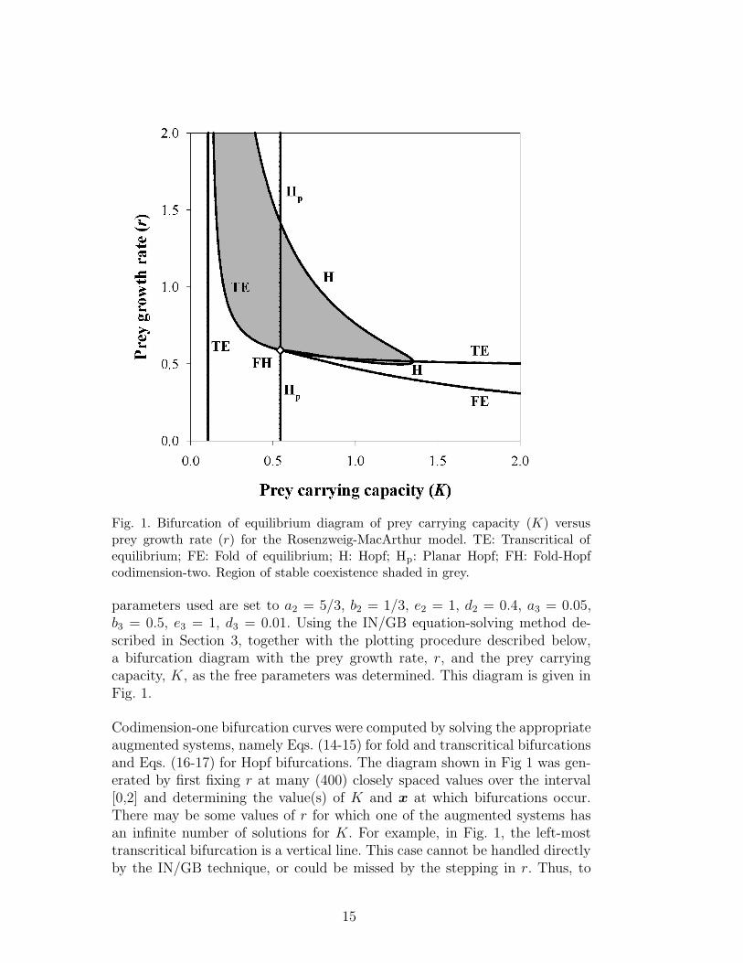
Fig. 1. Bifurcation of equilibrium diagram of prey carrying capacity (K) versusprey growth rate (r) for the Rosenzweig-MacArthur model. TE: Transcritical ofequilibrium; FE: Fold of equilibrium; H: Hopf; Hp: Planar Hopf; FH: Fold-Hopfcodimension-two. Region of stable coexistence shaded in grey.

parameters used are set to a2 = 5/3, b2 = 1/3, e2 = 1, d2 = 0.4, a3 = 0.05,b3 = 0.5, e3 = 1, d3 = 0.01. Using the IN/GB equation-solving method de-scribed in Section 3, together with the plotting procedure described below,a bifurcation diagram with the prey growth rate, r, and the prey carryingcapacity, K, as the free parameters was determined. This diagram is given inFig. 1.

Codimension-one bifurcation curves were computed by solving the appropriateaugmented systems, namely Eqs. (14-15) for fold and transcritical bifurcationsand Eqs. (16-17) for Hopf bifurcations. The diagram shown in Fig 1 was gen-erated by first fixing r at many (400) closely spaced values over the interval[0,2] and determining the value(s) of K and x at which bifurcations occur.There may be some values of r for which one of the augmented systems hasan infinite number of solutions for K. For example, in Fig. 1, the left-mosttranscritical bifurcation is a vertical line. This case cannot be handled directlyby the IN/GB technique, or could be missed by the stepping in r. Thus, to

15

ensure that all bifurcations are found, it is necessary to also scan in the K di-rection. That is, IN/GB was used to solve the appropriate augmented systemsfor r and x for many (400) closely spaced values of K over the interval [0,2].Codimension-two bifurcations were located by using IN/GB to solve the aug-mented system given by Eqs. (19-21) for K, r, and x. The bifurcation diagram(Fig. 1) computed using the interval method is consistent with the known Kversus r bifurcation diagram given by Gragnani et al. (1998), thus confirmingthe utility and accuracy of this method for determining bifurcation of equilib-ria diagrams. Such diagrams can be very easily and automatically generatedusing the IN/GB approach, with certainty that all bifurcation curves havebeen found.

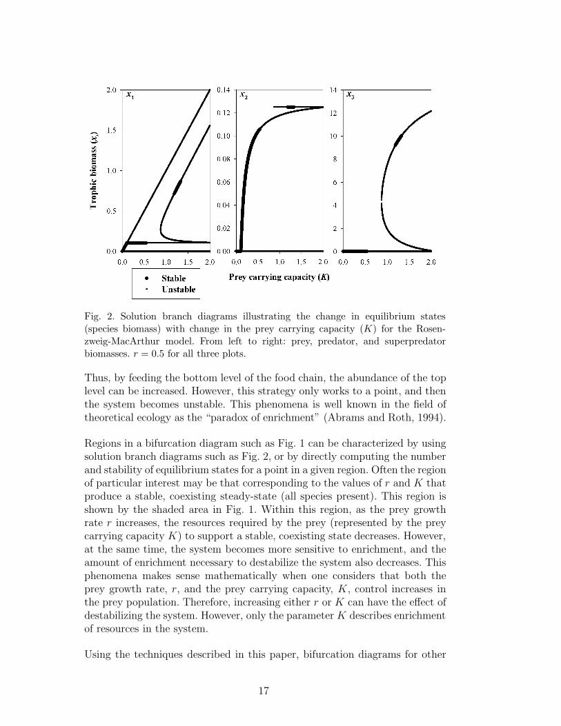
Another useful type of diagram in nonlinear dynamics is the solution branchdiagram (or one-parameter bifurcation diagram). This type of diagram showshow the steady-state values and stability of the state variables change as asingle model parameter is varied. These diagrams are also very easily generatedusing the interval method. For example, Fig. 2 shows how the equilibriumstates change as the prey carrying capacity, K, is varied from 0 to 2, whilethe prey growth rate, r, is held constant at a value of 0.5. This diagram wascomputed by using IN/GB to solve the nonlinear equation system given byEq. (12). This system was solved for many (2000) closely spaced values of K.In Fig. 2, and in subsequent solution branch diagrams, thin lines representunstable equilibria while thick lines represent stable equilibria.

In the solution branch diagram, one can observe several bifurcations of equilib-ria as K is increased. This can also be seen by following a horizontal line acrossFig. 1 at a value of r = 0.5. Moving to the right along this line, five bifurca-tions are encountered, namely (and in order) TE, Hp, FE, H, H (the rightmostTE is not crossed at r = 0.5). The first bifurcation to occur is a transcriti-cal bifurcation (K ≈ 0.105), in which a stable prey-only state collides witha prey-predator state which becomes feasible at the bifurcation. These statesexchange stability. The predator biomass then begins to increase while theprey biomass remains constant. The next bifurcation that is observed is a pla-nar Hopf bifurcation (K ≈ 0.544). Since this bifurcation occurs at an r valuebelow the fold-Hopf codimension-two bifurcation, this planar Hopf bifurcationdoes result in a change in stability in the model. Above the fold-Hopf point,the prey-predator state is feasible but is unstable due to the sign of the thirdeigenvalue, and thus the planar Hopf bifurcation does not result in a change ofstability. The next bifurcation to occur is a fold bifurcation (K ≈ 0.872) wheretwo unstable coexisting (prey-predator-superpredator) states become feasible.The next two bifurcations to occur are both Hopf bifurcations (K ≈ 1.186 andK ≈ 1.329). In the first Hopf bifurcation, one of the coexisting states becomesstable, and the same state become unstable in the subsequent bifurcation. Inthe narrow interval of K that produces a stable, coexisting steady state, in-creasing the prey carrying capacity increases the biomass of the superpredator.

16

Fig. 2. Solution branch diagrams illustrating the change in equilibrium states(species biomass) with change in the prey carrying capacity (K) for the Rosen-zweig-MacArthur model. From left to right: prey, predator, and superpredatorbiomasses. r = 0.5 for all three plots.

Thus, by feeding the bottom level of the food chain, the abundance of the toplevel can be increased. However, this strategy only works to a point, and thenthe system becomes unstable. This phenomena is well known in the field oftheoretical ecology as the “paradox of enrichment” (Abrams and Roth, 1994).

Regions in a bifurcation diagram such as Fig. 1 can be characterized by usingsolution branch diagrams such as Fig. 2, or by directly computing the numberand stability of equilibrium states for a point in a given region. Often the regionof particular interest may be that corresponding to the values of r and K thatproduce a stable, coexisting steady-state (all species present). This region isshown by the shaded area in Fig. 1. Within this region, as the prey growthrate r increases, the resources required by the prey (represented by the preycarrying capacity K) to support a stable, coexisting state decreases. However,at the same time, the system becomes more sensitive to enrichment, and theamount of enrichment necessary to destabilize the system also decreases. Thisphenomena makes sense mathematically when one considers that both theprey growth rate, r, and the prey carrying capacity, K, control increases inthe prey population. Therefore, increasing either r or K can have the effect ofdestabilizing the system. However, only the parameter K describes enrichmentof resources in the system.

Using the techniques described in this paper, bifurcation diagrams for other

17

Fig. 3. Bifurcation of equilibrium diagram of predator death rate (d2) versus preygrowth rate (r) for the Rosenzweig-MacArthur model with K = 1.0 TE: Tran-scritical of equilibrium; FE: Fold of equilibrium; H: Hopf; Hp: Planar Hopf; FH:Fold-Hopf codimension-two. Region of stable coexistence shaded in grey.

model parameters can be generated with ease. Similarly, it is also easy todetermine bifurcation diagrams for variations of the Rosenzweig-MacArthurmodel in which other predator response functions (e.g., sigmoidal or Hollingtype III) are used. Several such bifurcation diagrams have been computedusing the interval method by Gwaltney et al. (2004). One of these will bediscussed here so that comparisons can be made with the other models usedas examples. This is the bifurcation diagram for the Rosenzweig-MacArthurmodel with the prey growth rate r and predator death rate d2 as bifurca-tion parameters, and K = 1. This diagram was determined using the IN/GBapproach and is shown in Fig. 3.

Using solution branch diagrams to characterize the regions in Fig. 3 showsthat the rightmost transcritical bifurcation, which is a vertical line, forms theboundary between a stable prey-predator system (on the left) and a stableprey-only system (on the right). Moving to the left, the next transcriticalbifurcation curve intersects a codimension-two fold-Hopf point. At d2 values

18

to the right of the fold-Hopf point, this transcritical bifurcation is the boundarybetween the stable coexisting steady state and the stable prey-predator state.After the transcritical line intersects the fold-Hopf point, three bifurcationcurves are formed. These are a fold bifurcation, a transcritical bifurcation,and a Hopf bifurcation. The fold bifurcation is a horizontal line (r ≈ 0.46875)that originates at the fold-Hopf bifurcation. When increasing r and crossingthis fold bifurcation, two coexisting states form. Whether the transcriticalbifurcation or the Hopf bifurcation is crossed next depends on the value of d2.Crossing the transcritical bifurcation results in one of the two coexisting statesbecoming infeasible. The state that becomes infeasible is also unstable. Theother state formed in the fold bifurcation becomes stable in the region aboveand to the right of the Hopf bifurcation emanating from the fold-Hopf point.With this knowledge, we have an understanding of the region of coexistingstability in the d2 versus r parameter space. This region is shown by theshaded area in Fig. 3. The shape of the region of coexisting stability indicatesthat as the predator death rate, d2, increases, the minimum prey growth ratenecessary to support a stable system will first decrease up to the codimension-two fold-Hopf point, then increase. Furthermore, at larger prey growth rates,the system will tolerate higher predator death rates before the coexisting statebecomes infeasible. Finally, it is clear that there is an optimal prey growth ratethat will support the widest range of predator death rates.

4.2 Canale’s Chemostat Model

The second food chain model used as an example here is Canale’s chemostatmodel, as described in Section 2.2. Following Gragnani et al. (1998), the pa-rameters used are set to a1 = 1.25, b1 = 8, e1 = 0.4, d1 = 0.01, ε1 = 1,a2 = 0.33, b2 = 9, e2 = 0.6, d2 = 0.001, ε2 = 0.8, a3 = 0.021, b3 = 15.19,e3 = 0.9, d3 = 0.0001, ε3 = 0.1. A bifurcation diagram with the inflow rate, D,and the concentration of the nutrient in the inflow, xn, as the free parameterswas then computed using the IN/GB method. This diagram is shown in Fig.4.

The codimension-one bifurcation curves were computed by solving the appro-priate equation systems (see Section 2.5), first fixing xn at many (400) closelyspaced values over the interval [0,400] and determining the value(s) of D andx at which bifurcations occur, and then fixing D at many (700) closely spacedvalues over the interval [0,0.14] and determining the value(s) of xn and x atwhich bifurcations occur. A single codimension-two (fold-Hopf) bifurcationwas located by solving the appropriate augmented system for xn, D, and x.

Fig. 4 captures all bifurcations of equilibria shown in the D vs. xn bifurcationdiagram presented by Gragnani et al. (1998). However, Fig. 4 also shows other

19

Fig. 4. Bifurcation of equilibrium diagram of nutrient inflow concentration (xn) ver-sus inflow rate (D) for Canale’s chemostat model. TE: Transcritical of equilibrium;FE: Fold of equilibrium; H: Hopf; Hp: Planar Hopf; FH: Fold- Hopf codimension-two.Region of stable coexistence shaded in grey.

bifurcation curves that do not appear in Gragnani et al.’s diagram. First, thereis a transcritical bifurcation curve very near the D axis (the leftmost TE in Fig.4) that is not given by Gragnani et al. At this bifurcation, a stable nutrient-only equilibrium state collides with an infeasible nutrient-prey equilibriumstate; the nutrient-prey state becomes feasible and exchanges stability withthe nutrient-only state. Second, there is a planar Hopf bifurcation curve nearthe xn axis (lowest Hp in Fig. 4) that is not shown by Gragnani et al. (we havealso computed other planar Hopf bifurcations curves very near the xn axis,but these are not visible in Fig. 4 due to the scale used). For all of these Hp

bifurcations, the stability change occurs only in a two-variable subspace, withthe stability of the overall system remaining unchanged (unstable); this is alsothe case for the lower portion (beneath the fold-Hopf point) of the planar Hopfcurve that intersects the fold-Hopf point, which appears both in Fig. 4 andin Gragnani et al.’s diagram. Whether the planar Hopf curves omitted fromGragnani et al.’s diagram were actually not found, or were omitted simplybecause they were not considered interesting, is not clear. What is important

20

Fig. 5. Solution branch diagrams illustrating the change in equilibrium states(species biomass) with change in the nutrient concentration of the inflow (xn) forCanale’s chemostat model. From left to right: prey, predator, and superpredatorbiomasses. D = 0.09 for all three plots.

here is that, by using the IN/GB method, we can say with complete confidencethat we have in fact found all of the bifurcations curves of interest.

Fig. 5 tracks the behavior of the equilibrium states as xn is increased from0 to 400 along the horizontal line D = 0.09 in Fig. 4. Moving to the rightalong this line, seven bifurcations are encountered, namely (and in order)TE, TE, Hp, FE, TE, H, H. The first TE is not clearly visible in Fig. 5due to the scale used. The sixth and seventh bifurcations, both Hopf, are ofparticular interest here. The sixth bifurcation (xn ≈ 112.5) results in the firststable, coexisting steady-state (all three species present). But at the seventhbifurcation (xn ≈ 184.5), this state becomes unstable. However, within thisregion of stability increasing the inflow nutrient concentration, xn, enrichesthe food chain and increases the stable population of the top predator, butonly to a point. This again illustrates the “paradox of enrichment” in thatbeyond the second Hopf bifurcation the system becomes unstable and thepopulations may experience “boom and bust” cycles. This behavior is verysimilar to the behavior observed in Fig. 2, which indicates that, while theRosenzweig-MacArthur model does not explicitly account for resources, it canproduce similar behavior when compared to a resource-based model, such asCanale’s model.

Using solution branch diagrams like Fig. 5 we can characterize the regions in

21

Fig. 4 and identify the bounds on the region of xn and D that corresponds toa stable, coexisting steady-state. This region is shown by the shaded area inFig. 4. As indicated in Fig. 4, as the inflow rate, D, increases, the minimuminflow nutrient concentration, xn, required to support a coexisting steady-statealso increases. This behavior is intuitive because, as the inflow rate increases,more nutrient and organisms are washed out of the system, resulting in theneed for a higher nutrient inflow concentration, xn, to support the minimumbiomasses of prey and predators necessary for survival of the predators andsuperpredators, respectively.

The maximum xn boundary for the region supporting a stable, coexistingsteady state of all three species is the rightmost Hopf bifurcation curve. Atxn values to the of right this curve, the system is over-enriched and losesstability. One can thus see from Fig. 4 that at relatively low inflow rates(D / 0.0414), increasing D causes the maximum xn allowable for a stablecoexisting state to decrease. This can be explained by recognizing that at verylow values of the inflow rate, D, increasing the inflow rate has the predominanteffect of increasing the addition of nutrients to the system, thereby leading toover-enrichment and decreasing the inflow nutrient concentration at whichthe rightmost Hopf bifurcation occurs in Fig. 4. However, at values of D '0.0414, increasing the inflow rate causes the effects of washout to become morepronounced, and larger values of xn are allowable because of the high removalrate of both biomass and system nutrient.

Various authors have utilized bifurcation diagrams to make comparisons be-tween different food chain model formulations. Kooi et al. (1997b, 1998) com-pared several different formulations of chemostat-based food chain models.These authors used model formalisms to compare simple formulations withtwo state variables, while models with three or four state variables were com-pared using bifurcation diagrams. These latter models are similar in formu-lation to the Rosenzweig-MacArthur model and Canale’s chemostat model,as studied here and by Gragnani et al. (1998), however a different set of pa-rameters was used. Kooi et al. (1997b, 1998) concluded that chemostat-basedmodels exhibited fundamentally different behavior than models with prey thatgrow according to the logistic growth function. On the other hand, Gragnaniet al. (1998) compared the Rosenzweig-MacArthur model (logistic prey) withCanale’s chemostat model under conditions of enrichment, and concluded thatthe two models produce the same dynamics when a key parameter is var-ied. That is, the dynamics observed when K was varied in the Rosenzweig-MacArthur model were equivalent to those in Canale’s model when xn wasvaried. Since Kooi et al. (1997b, 1998) and Gragnani et al. (1998) studied sys-tems under much different conditions (model parameters), these conclusionsare not necessarily in conflict.

In this work, we can compare the shaded region in Fig. 4 with the region pro-

22

ducing a stable, coexisting steady state for the Rosenzweig-MacArthur model(Fig. 1). This comparison indicates that these regions are dissimilar. That is,the behavior observed when changing both r and K is not equivalent to thebehavior observed when changing both D and xn. This is due to inconsis-tencies between the parameters compared in these models. The prey growthrate r in the Rosenzweig-MacArthur model is not equivalent to the systeminflow rate D in Canale’s model. Thus, the use of a different parameter setin the analysis of Canale’s chemostat model may be appropriate for makingcomparisons of behavior with the Rosenzweig-MacArthur model. Since theRosenzweig-MacArthur model does not explicitly account for resources or forwashout, there is no parameter in that model that is equivalent to D. How-ever, in Canales model, the prey species grows at a maximum rate of e1a1;thus changing the maximum nutrient consumption rate by the prey, a1, shouldhave a similar effect to changing the prey growth rate r in the Rosenzweig-MacArthur model. Using IN/GB and the techniques described above, it is arelatively easy matter to generate a bifurcation diagram in the xn vs. a1 pa-rameter space. This diagram appears as Fig. 6. Since Fig. 4 and Fig. 6 sharea common parameter (xn), the figures should intersect in a three-dimensionalparameter space. In fact, the bifurcations that occur along the lines D = 0.07in Fig. 4 and a1 = 1.25 in Fig. 6 occur in the same order and at the samevalues. This fact makes classification of some of the bifurcation lines mucheasier.

Comparison of Fig. 6 for Canale’s model and Fig. 1 for the Rosenzweig-MacArthur model shows clear similarities. There are differences, including anadditional transcritical bifurcation (which must exist due to the extra statevariable x0) and the general shape of the bifurcation curves. However, theorder in which one crosses these curves, whether moving from left to right, ortop to bottom, is the same in both diagrams. The region in Fig. 6 in whichthere is a stable, coexisting steady state is shown by the shaded area. Thisregion is very similar in shape to the region of steady, stable coexistence inFig. 1. The behavior observed is very similar to the behavior discussed in Sec-tion 4.1 in that, as a1 increases, the amount of food required by the prey, xn,to support a stable, coexisting state decreases. However, at the same time,increasing a1 also causes the system to become more sensitive to enrichment,and thus the amount of enrichment necessary to destabilize the system alsodecreases. The most noticeable differences between Fig. 6 and Fig. 1 pertainmainly to lines controlling the feasibility and stability of trophic subsystemsin the models, such as the nutrient-prey-predator system in Canale’s modeland the prey-predator system in the Rosenzweig-MacArthur model. The qual-itative behavior in the region of stable coexistence is very similar in bothmodels.

We can make a similar comparison by using the IN/GB method to gener-ate an a1 versus d2 bifurcation diagram for Canale’s model. This diagram,

23

Fig. 6. Bifurcation of equilibrium diagram of nutrient inflow concentration (xn) ver-sus maximum nutrient consumption rate by the prey (a1) for Canale’s chemostatmodel with D = 0.07. TE: Transcritical of equilibrium; FE: Fold of equilibrium; H:Hopf; Hp: Planar Hopf; FH: Fold-Hopf codimension-two. Region of stable coexis-tence shaded in grey.

given in Fig. 7, can be compared to the to the r versus d2 diagram for theRosenzweig-MacArthur model (Fig. 3). In Fig. 7, several of the bifurcationcurves lie very close together. Following a vertical line in Fig. 7 (increasinga1) at the value of the predator death rate used by Gragnani et al. (1998)(d2 = 0.001), we encounter seven bifurcations, namely (and in order): TE,TE, Hp, FE, H, H, TE. Initially the system has only one steady-state, whichis a stable nutrient-only state. At a1 values below the horizontal transcriticalbifurcation (a1 = 0.208), the prey does not consume nutrient quickly enoughfor a nutrient-prey state to be feasible. In the first transcritical bifurcation, anutrient-prey state forms, collides, and exchanges stability with the nutrient-only state. In the second transcritical bifurcation, a nutrient-prey-predatorsystem becomes feasible and exchanges stability with the nutrient-prey state.Then, as the planar-Hopf bifurcation is crossed, the nutrient-prey-predatorstate loses stability. Due to the proximity of these three bifurcation lines atlow values of the predator death rate, the transition from a condition where

24

Fig. 7. Bifurcation of equilibrium diagram of predator death rate (d2) versus maxi-mum nutrient consumption rate by the prey (a1) for Canale’s chemostat model withD = 0.07 and xn = 200.0. TE: Transcritical of equilibrium; FE: Fold of equilibrium;H: Hopf; Hp: Planar Hopf; FH: Fold-Hopf codimension-two. Region of stable coex-istence shaded in grey.

the only feasible state is the (stable) nutrient-only state to a condition wherethere are three feasible states, none of which are stable, occurs over a verysmall range of a1. As the maximum nutrient consumption rate (a1) is furtherincreased a fold bifurcation is crossed, which causes two coexisting states tobecome feasible, but neither are stable. This fold bifurcation is, in fact, a hor-izontal line with a value of a1 ≈ 0.487. The behavior of this fold bifurcation isqualitatively identical to that observed in Fig. 3. The presence of a horizontalfold bifurcation marking the boundary for coexisting feasibility indicates thatthe prey growth rate r in the Rosenzweig-MacArthur model, and the maximumnutrient consumption rate a1 in Canale’s model are comparable parameters,and they have very similar effects on system behavior. Furthermore, it indi-cates that there is a minimum r or a1 below which the prey simply cannotgrow fast enough to replace losses and maintain a feasible, coexisting steadystate, and that this minimum value is independent of the predator death rated2. The Hopf bifurcation, which originates in the fold-Hopf codimension-two

25

bifurcation, is crossed next. When this bifurcation is crossed, one of the coex-isting states becomes stable. The fold bifurcation and Hopf bifurcation occurat extremely close values of a1, which results in the two lines being almostindistinguishable on Fig. 7. Crossing the second Hopf bifurcation (which en-ters the diagram on the a1 axis) causes the stable coexisting state to becomeunstable. Crossing the subsequent transcritical bifurcation causes the unsta-ble coexisting state that did not change stability due to the Hopf bifurcationto become infeasible. This transcritical bifurcation, which emanates from thefold-Hopf codimension-two point, causes the same change in system behavioras the transcritical line emanating from the fold-Hopf point in Fig. 3.

With this knowledge, we can visualize the region of coexisting feasibility andstability. This region is shown by the shaded area in Fig. 7. The transcriticalbifurcation that intersects the fold-Hopf bifurcation forms the right boundaryof steady, stable coexistence at predator death rate values greater than thecodimension-two fold-Hopf bifurcation (d2 ≈ 0.0955). To the right of this tran-scritical bifurcation the predator death rate is too large and the superpredatorpopulation is decimated. This behavior is also identical to that observed inFig. 3. Thus, at some point no matter how quickly the prey are able to growand replace their losses, increasing the predator death rate will cause a stablecoexisting steady-state to become infeasible. This macroscopic change occurswhen the superpredator population disappears, not the predator population,even though it is the predator death rate that is increasing. While this behav-ior is counterintuitive, as explained in Gwaltney et al. (2004), similar behaviorcan also be seen in the Rosenzweig-MacArthur model.

As indicated by the shaded areas, the regions in Fig. 3 and Fig. 7 supportinga stable, coexisting steady-state are very similar in shape. The primary differ-ence is that in Fig.7, the Hopf bifurcation line emanating from the fold-Hopfbifurcation does not reverse direction. Instead, moving to the left, it crossesthe a1 axis. Another Hopf bifurcation then enters the diagram on the a1 axis,and this Hopf bifurcation causes the same change in stability that is causedby the Hopf bifurcation in Fig. 3 after it changes direction. Actually, if Fig.7 were extended into the negative d2 parameter space, we could see that thetwo Hopf bifurcations are actually a continuous curve that reverses direction,just like in Fig. 3. The key bifurcation lines that control the feasibility of thecoexisting state are identical in behavior to those observed in Fig. 3. In gen-eral, as the maximum nutrient consumption rate by the prey, a1, increases, thesystem given by Canale’s Chemostat model is able to tolerate higher predatordeath rates before the coexisting state becomes infeasible. In Canale’s modelwe also observe that as the maximum nutrient consumption rate by the preyincreases, the minimum predator death rate necessary to support a stable co-existing state increases. This behavior matches the behavior observed in Fig.3 for the Rosenzweig-MacArthur model.

26

The primary differences between Fig. 7 for Canale’s model and Fig. 3 forthe Rosenzweig-MacArthur model are seen in the bifurcation lines which dealwith the boundaries at which the predator population becomes infeasible,and where the prey-predator subsystem changes stability. These lines are theplanar Hopf bifurcation and the rightmost transcritical bifurcation in Figs.3 and 7. An additional horizontal transcritical bifurcation is present in Fig.7. The presence of this bifurcation is expected as it provides the boundarybetween the nutrient-only state and the nutrient-prey state. The fact thatthe line is horizontal indicates that the minimum value of a1 necessary tosupport a feasible (and stable) nutrient-prey state does not depend on thepredator death rate, d2. This behavior is expected because the behavior of thenutrient-prey subsystem should not depend on any parameters not appearingin the subsystem, including the predator death rate. We will observe identicalbehavior in examining the algae-rotifer model, which is also explicitly accountsfor resources by modeling the limiting nutrient in a chemostat.

4.3 Algae-Rotifer Model

The final food chain model used as an example here is the algae-rotifer model,as described in Section 2.3. Following Fussmann et al. (2000), the parame-ters used are set to bC = 3.3 day−1, KC = 4.3 µmol/liter, bB = 2.25 day−1,KB = 15 µmol/liter, m = 0.055 day−1, λ = 0.4 day−1, and ε = 0.25. The fourstate variables (N , C, R and B) are modeled in terms of nitrogen concen-tration (µmol/liter), with the last three then converted to numbers of organ-isms according to 1 µmol/liter = 5 × 104 cells per milliliter for Chlorella and1 µmol/liter = 5 females per milliliter for Brachionus. A bifurcation diagramwith the inflow rate, δ, and the concentration of the nitrogen in the inflow,Ni, as the free parameters was then computed using the IN/GB method, andis given in Fig. 8.

Fussmann et al. (2000) determined a δ vs. Ni bifurcation diagram by usinga grid-based approach in which a grid is established in the two-variable pa-rameter space and the number and stability of equilibrium states is computeddirectly at each grid point. In comparing Fig. 8 to the diagram presented byFussmann et al. (2000), one should note that the axes have been reversed in or-der to facilitate comparisons with the models previously discussed in this work.Furthermore, the diagram presented by Fussmann et al. (2000) contained aregion for the coexistence of stable limit cycles, which are not examined in thiswork. Finally, Fig. 8 shows a transcritical bifurcation along the inflow rate (δ)axis, which does not appear in Fussmann et al. (2000). This occurs becausethe diagram in Fussmann et al. (2000) is limited to defining regions in whicha stable, coexisting state exists (whether it is an equilibrium state or a limitcycle).

27

Fig. 8. Bifurcation of equilibrium diagram of inflow nitrogen concentration (Ni)versus inflow rate (δ) for the algae-rotifer model. TE: Transcritical of equilibrium;H: Hopf. Region of stable coexistence shaded in grey.

In Fig. 8, as Ni increases, in most cases three bifurcations will be crossed, andthese are (from left to right) two transcritical bifurcations and a Hopf bifurca-tion. At values of δ / 0.037, another Hopf bifurcation will also be crossed. Asthe leftmost transcritical bifurcation is crossed, a stable nitrogen-algae systembecomes feasible. As the second transcritical bifurcation is crossed, a stablecoexisting (nitrogen-algae-rotifer) state becomes feasible (and the nitrogen-algae system becomes unstable). Finally, as the Hopf bifurcation is crossed,the stable coexisting state becomes unstable. Crossing the Hopf bifurcationnear the Ni axis also causes the stable coexisting state to become unstable. Ata given value of Ni, at values of δ below this Hopf bifurcation, the coexistingstate is feasible, but unstable.

The region where a coexisting steady-state is both feasible and stable is shownby the shaded area in Fig. 8. When comparing Fig. 8 with Fig. 4, one mayinitially notice a similarity between the regions of steady, stable coexistence.However, recall that the algae-rotifer model only features two trophic levels,while Canale’s model features three. Thus, the rightmost transcritical and

28

Hopf bifurcations in Fig. 8 are equivalent to the middle transcritical bifurcationand the planar Hopf bifurcation passing through the fold-Hopf point in Fig.4. Even taking this into account, the behavior of the stable, coexisting state(nitrogen-algae-rotifer) in the algae-rotifer model matches the same trendsobserved in the nutrient-prey-predator subspace of Canale’s chemostat model.There is one primary difference, that being that the lower boundary in Fig. 4is formed by the transcritical bifurcation (which also forms the left boundary)while in Fig. 8, the lower boundary consists of a Hopf bifurcation. Despitethis difference, it should be recognized that increasing the dilution rate (δ)or the nitrogen concentration in the inflow medium (Ni) has a similar effectto increasing either D or xn on the nutrient-prey-predator state in Canale’schemostat model. Thus these models exhibit similar behavior in terms of theeffects of enrichment, and the paradox of enrichment also applies to the algae-rotifer model.

In order to further compare the algae-rotifer model with both the Rosenzweig-MacArthur model and Canale’s chemostat model, a bifurcation diagram com-paring the maximum algal growth rate, bC , and the inflow medium nitrogenconcentration, Ni, is needed. It is easy to reliably generate this diagram usingthe IN/GB method and the techniques described in this paper. The bifurcationdiagram is given in Fig. 9.

This diagram can be compared to Fig. 1 for the Rosenzweig-MacArthur modeland Fig. 6 for Canale’s chemostat model. The bifurcation curves are easilyidentifiable because along the lines δ = 0.08 day−1 and bC = 3.3 day−1, Fig. 8and Fig. 9 intersect. Thus, the order of the bifurcation curves is, from left toright, and bottom to top, TE, TE, H. The region of steady, stable coexistenceis shown by the shaded area in Fig. 9. Initially this region seems dissimilarto the regions observed in Fig. 1 and Fig. 4. Recall that in the Rosenzweig-MacArthur model and in Canale’s chemostat model, as the prey growth rateincreased, the amount of enrichment needed to destabilize the coexisting statedecreased. The opposite effect is predicted by the algae-rotifer model. Thisphenomena is, again, explained by the fact that the algae-rotifer model con-sists of only two trophic levels, while the other two models both feature threetrophic levels. The rightmost transcritical and Hopf bifurcation curves in Fig.9 can be thought of as being equivalent to the middle transcritical bifur-cation and the planar Hopf bifurcation in Fig. 6. Thus the behavior of thecoexisting state (nitrogen-algae-rotifer) of the algae-rotifer model matches thebehavior observed in the nutrient-prey-predator subspace of Canale’s model.The behavior of these spaces differs from the Rosenzweig-MacArthur modelin that the limits of steady, stable coexistence for the prey-predator subspacein the Rosenzweig-MacArthur model do not depend on the prey growth rate,r, which can observed by the vertical planar Hopf bifurcation line and thevertical (leftmost) transcritical bifurcation in Fig. 1.

29

Fig. 9. Bifurcation of equilibrium diagram of inflow nitrogen concentration (Ni)versus maximum algal growth rate (bC) for the algae-rotifer model with δ = 0.8/day.TE: Transcritical of equilibrium; H: Hopf. Region of stable coexistence shaded ingrey.

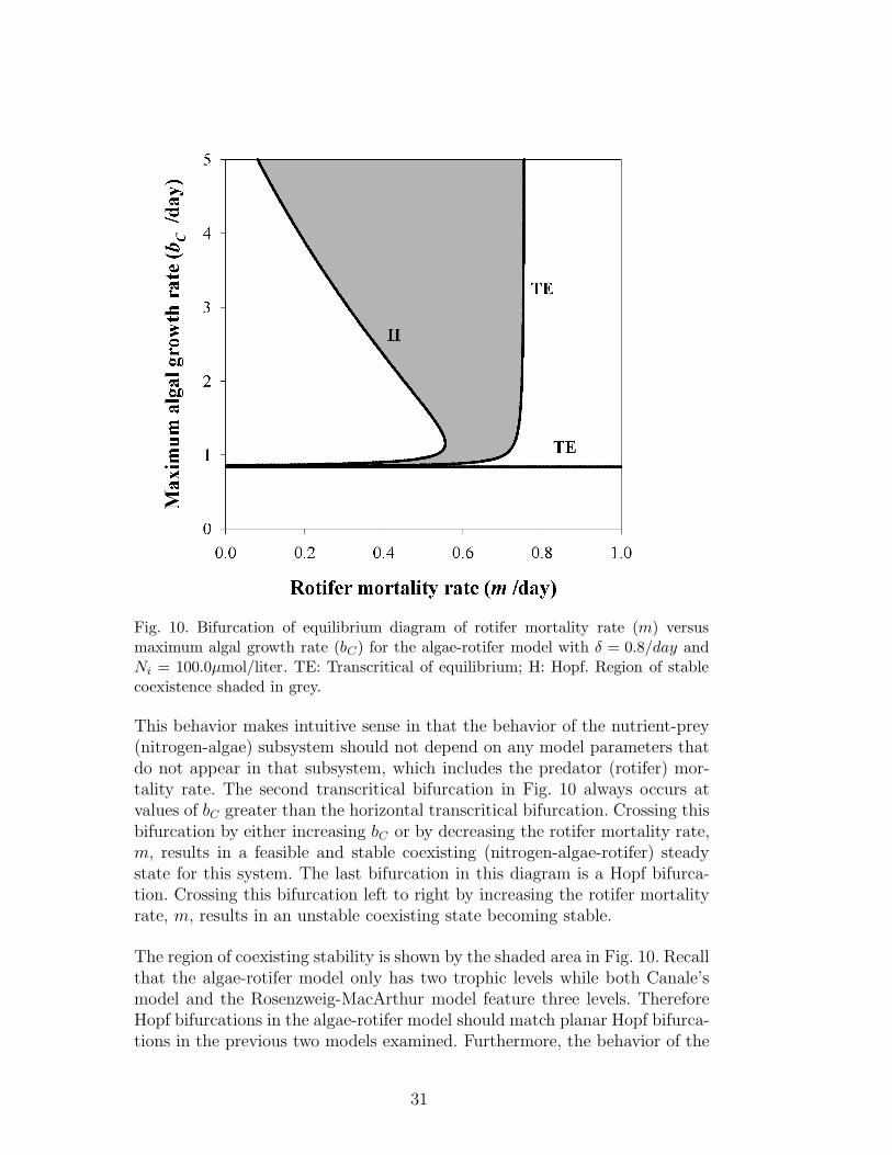
In order to compare the behavior predicted by the experimentally-verifiedalgae-rotifer model with the behaviors predicted by the Rosenzweig-MacArthurmodel in Fig. 3 and by Canale’s model in Fig. 7, a diagram comparing themaximum algal growth rate, bC , with the rotifer mortality rate, m, is neces-sary. This diagram was generated using the IN/GB method, as before, and isgiven in Fig. 10.

In Fig. 10 there are three bifurcation curves present. There is a horizontaltranscritical line at bC ≈ 0.8344, which matches the value of bC at which thetranscritical bifurcation occurs in Fig. 9 at Ni = 100.0. At values of bC belowthis line, the only feasible state is a nutrient-only state. Crossing this tran-scritical bifurcation results in a nitrogen-algae state becoming both feasibleand stable. This horizontal line in Fig. 10 indicates that there is a minimumvalue of the maximum algal growth rate bC that is necessary to support afeasible algal population, and this value is not dependent on the rotifer mor-tality rate, which matches the behavior observed in Canale’s model in Fig. 7.

30

Fig. 10. Bifurcation of equilibrium diagram of rotifer mortality rate (m) versusmaximum algal growth rate (bC) for the algae-rotifer model with δ = 0.8/day andNi = 100.0µmol/liter. TE: Transcritical of equilibrium; H: Hopf. Region of stablecoexistence shaded in grey.

This behavior makes intuitive sense in that the behavior of the nutrient-prey(nitrogen-algae) subsystem should not depend on any model parameters thatdo not appear in that subsystem, which includes the predator (rotifer) mor-tality rate. The second transcritical bifurcation in Fig. 10 always occurs atvalues of bC greater than the horizontal transcritical bifurcation. Crossing thisbifurcation by either increasing bC or by decreasing the rotifer mortality rate,m, results in a feasible and stable coexisting (nitrogen-algae-rotifer) steadystate for this system. The last bifurcation in this diagram is a Hopf bifurca-tion. Crossing this bifurcation left to right by increasing the rotifer mortalityrate, m, results in an unstable coexisting state becoming stable.

The region of coexisting stability is shown by the shaded area in Fig. 10. Recallthat the algae-rotifer model only has two trophic levels while both Canale’smodel and the Rosenzweig-MacArthur model feature three levels. ThereforeHopf bifurcations in the algae-rotifer model should match planar Hopf bifurca-tions in the previous two models examined. Furthermore, the behavior of the

31

coexisting state in the algae-rotifer model should match the behavior of theprey-predator subspace in the other two models. When Fig. 10 is comparedto Fig. 7 we can immediately see that the behavior of the Hopf bifurcationin Fig. 10 matches the behavior of the planar Hopf bifurcation in Fig. 7.Crossing the planar Hopf bifurcation in Fig. 7 results in a change in stabil-ity of the nutrient-prey-predator subsystem; however, this stability change isnot always observed due to the sign of the fourth eigenvalue. Furthermore,the second (non-horizontal) transcritical bifurcation in Fig. 10 matches thebehavior of the rightmost transcritical bifurcation in Fig. 7. Therefore, thetrends observed for the nutrient-prey-predator system are equivalent in thetwo models. In the Rosenzweig-MacArthur model, once again we see that theprey-predator subspace is bounded by a vertical planar Hopf bifurcation lineand a vertical (rightmost) transcritical bifurcation in Fig. 3, and therefore thisregion, as observed previously, does not depend on the prey growth rate, r.This, of course, differs from the behavior observed for both Canale’s modeland the algae-rotifer model. However, it is easy to see that the two chemostat-based models behave quite similarly when the comparison is made betweenidentical state spaces.

5 Concluding Remarks

Using several examples drawn from three different food chain models, we havedemonstrated here the use of an interval-Newton method for the analysis ofthe nonlinear dynamical systems that arise in food chain modeling, specificallyfor computing all equilibrium states and bifurcations of equilibria (fold, tran-scritical, Hopf, double-fold and fold-Hopf). Using this method it was possibleto easily, without any need for initialization or a priori insight into expectedsystem behavior, generate complete solution branch diagrams and bifurcationof equilibria diagrams. This was done automatically, without requiring userinteraction, a common need (Kuznetsov, 1998) in using continuation tools.Furthermore, this could be done with certainty, since the technique providesa mathematical and computational guarantee that all solutions to a systemof nonlinear equations are enclosed. Since this technique is essentially initial-ization independent, beyond the setting of an initial interval for study, it canprovide a powerful alternative to traditional continuation methods, which ingeneral are initialization dependant and thus may not be completely reliable.

In principle, the interval method can be applied to compute the equilibriumstates and bifurcations of equilibria in any continuous-time model of popula-tion dynamics in a food chain or food web, though in practice it is subject tosome limitations, as discussed below. The advantages provided by the intervalapproach should make it particularly useful whenever analysis of a new modelis undertaken, since this is the case in which initialization issues are most likely

32

to arise in using traditional methods. For similar reasons, we have found themethod to be very useful, as shown in the examples above, in working withexisting models in parameter subspaces not analyzed previously.

We are particularly interested in the application of this method in the devel-opment and improvement of relatively small-scale food webs. There has beensignificant recent interest in modeling such systems and in studying their dy-namics using bifurcation analysis. For example, Kooi and Kooijman (2000)developed a simple food network model that illustrates the effects of introduc-ing a competitive species in the lowest trophic level. One- and two-parameterbifurcation diagrams in a parameter space describing the addition of nutrientsto the system were used to show that introducing a competitive species tothe prey trophic level can stabilize an oscillatory nutrient-prey-predator sys-tem. Kuijper et al. (2003) used a small-scale food web model to to investigatethe effects of omnivory, or intraguild predation, in a chemostat. Bifurcationdiagrams were computed to analyze the relationship between the extent ofintraguild predation and the concentration of nutrient in the inflow, showingthat omnivory can stabilize food chains, eliminate chaos, and give rise to mul-tiple steady states. Kavadia et al. (2007) studied the dynamics of free-living,nitrogen-fixing bacterial populations under varying environmental and com-petitive conditions using a simple food network model. Bifurcation diagramswere used to illustrate the effects of altering system dilution rates and en-ergy sources, with the conclusion that nitrogen-fixing populations can coexistwith competitors under certain conditions of enrichment, but can be inhib-ited or destroyed when specific nutrient resources are low. In these examples,and in similar small-scale food network models, the interval approach can beapplied to validate existing bifurcation diagrams and to compute new bifur-cation diagrams for other parameter values or in other parameter subspaces.By providing a reliable and very easily used approach for determining one- ortwo-parameter bifurcation diagrams, the interval method also makes it easyto look at the effects of changing trophic interactions and response functions,as well as parameter values, and to thus study possible improvements in themodels.

Despite the advantages of the interval technique described here, there aresome practical limitations. An important limitation is that our current imple-mentation of the interval-Newton method is not suitable for directly locatinglimit cycles and their bifurcations, which are very important dynamic features.By providing a reliable method for computing Hopf bifurcations, the intervalmethod does provide a reliable means to initialize continuation methods forlocating cycles (since a Hopf bifurcation corresponds to the appearance or dis-appearance of a limit cycle), and this is useful. This combination of intervaland continuation methods should provide a reliable, though not guaranteed ap-proach for locating limit cycles and their bifurcations. A fully interval methodfor limit cycles is being investigated, based in part on ideas provided by Galias

33

(2001, 2002).

Another limitation of the interval approach is in the problem size (number ofstate variables) that it can be applied to. This limitation is directly relatedto computation time requirements, and thus some discussion of the computa-tional effort required to solve the example problems is needed. Average CPUtimes for the computation of fold and transcritical bifurcations ranged from 0.6to 16 seconds per parameter iteration, while for computing Hopf bifurcationsthis figure was 1.4 to 100 seconds. Computing codimension-2 double fold andfold-Hopf bifurcation points required between 39 and 4800 seconds. The widerange of computation times is due to a variety of factors, including differencesin the level of complexity between the models, as well as differences betweencomputers used (all computations were done on either a 1.7 GHz or 3.4 GHz In-tel CPU, under the Linux operating system using Intel Fortran Compiler 7.1).For the examples studied here we consider this level of computational effort tobe quite reasonable, especially since the method used provides a guarantee ofreliability, which other methods do not. Furthermore, since the diagrams canbe generated automatically, without user intervention to deal with initializa-tion issues, the elapsed time to generate a bifurcation diagram for a new modelmay actually be significantly less than when initialization-dependent methodsare used. However, as problem size grows much beyond that considered here,the determination of two-parameter bifurcation diagrams using the intervalmethod will become significantly more expensive computationally. This is dueprimarily due to the complexity involved in computing the determinant andbialternate product functions, and their derivatives, in Eqs. (15), (17), (20)and (21). On the other hand, the computation of equilibrium states was ex-tremely fast for the models considered in this work, requiring less than 0.1seconds of CPU time per parameter iteration. This suggests that it should bepossible to compute solution branch diagrams for much larger systems. Wehave recently demonstrated this by using the interval method to compute allthe equilibrium states in a nonlinear 17-variable food web model Gwaltney etal. (2006).

6 Acknowledgments

This work was supported in part by the Department of Education Gradu-ate Assistance in Areas of National Needs (GAANN) Program under Grant#P200A010448, by the State of Indiana 21st Century Research and Technol-ogy Fund under Grant #909010455 and by the National Oceanic and Atmo-spheric Administration under Grant #NA050AR4601153.

34

References

Abrams, P.A., Roth, J.D., 1994. The effects of enrichment of three-speciesfood chains with non-linear functional responses. Ecology, 75, 1118–1130.

Bartell, S.M., Gardner, R., and O’Neill, R., 1992. Ecological Risk Estimation.Lewis Publishers, Ann Arbor, MI, 272 pp.

Bernot, R.J., Kennedy, E.E., Lamberti, G.A., 2005. Effects of ionic liquids onthe survival, movement, and feeding behavior of the freshwater snail, Physa

acuta. Environ. Toxicol. Chem., 24, 1759–1765.Bernot, R.J., Brueseke, M.A., Evans-White, M.A., Lamberti, G.A., 2005.

Acute and chronic toxicity of imidazolium-based ionic liquids on Daphnia

magna. Environ. Toxicol. Chem., 24, 87–92.Bischof, C.H., Lang, B., Marquardt, W., Monnigmann, M., 2000. Verified de-

termination of singularities in chemical processes. Proc. SCAN 2000, 9thGAMM-IMACS International Symposium on Scientific Computing, Com-puter Arithmetic, and Validated Numerics, Sept. 18-22, 2000, Karlsruhe,Germany.

Boer, M.P., Kooi, B.W., Kooijman, S.A.L.M, 1998. Food chain dynamics inthe chemostat. Math. Biosci., 150, 43–62.

Brennecke, J.F., Maginn, E.J., 2001. Ionic liquids: Innovative fluids for chem-ical processing. AIChE J., 47, 2384–2389.

De Feo, O., Rinaldi, S., 1997. Yield and dynamics of tritrophic food chains.Am. Nat., 150, 328–345.

Dhooge, A., Govaerts, W., Kuznetsov, Y.A., 2003. MATCONT: A MATLABpackage for numerical bifurcation analysis of ODEs. ACM Trans. Math.Softw., 29, 141–164.

Docherty, K.M, Kulpa, C.F., 2005. Toxicity and antimicrobial activity ofimidazolium and pyridinium ionic liquids. Green Chem., 7, 185–189.

Doedel, E.J., Paffenroth, R.C., Champneys, A.R., Fairgrieve, T.F.,Kuznetsov, Y.A., Oldeman, B.E., Sandstede, B., 2002. AUTO 2000:Continuation and bifurcation software for ordinary differential equa-tions (with HomCont). User’s Guide. Available with software athttp://sourceforge.net/projects/auto2000.

El-Sheikh, M.M.A., Mahrouf, S.A.A., 2005. Stability and bifurcation of a sim-ple food chain in a chemostat with removal rates. Chaos Solitons Fractals,23, 1475–1489.

Fussmann, G.F., Ellner, S.P., Shertzer, K.W., Hairston, N.G., 2000. Crossingthe Hopf bifurcation in a live predator-prey system. Science, 290, 1358–1360.

Galias, Z., 2001. Interval methods for rigorous investigation of periodic orbits.International Journal of Bifurcation and Chaos, 11, 2427–2450.

Galias, Z., 2002. Proving the existence of long periodic orbits in 1D mapsusing Interval-Newton method and backward shooting. Topology and itsApplications, 124, 25–37.

Gau, C.-Y., Stadtherr, M.A., 2002. New interval methodologies for reliablechemical process modeling. Comput. Chem. Eng., 26, 827–840.

35

Gehrke, V., Marquardt, W., 1997. A singularity theory approach to the studyof reactive distillation. Comput. Chem. Eng., 21(Suppl.), S1001–S1006.

Gorman-Lewis, D.J., Fein, J.B., 2004. Experimental study of the adsorption ofan ionic liquid onto bacterial and mineral surfaces. Environ. Sci. Technol.,38, 2491–2495.

Govaerts, W.J.F., 2000. Numerical Methods for Bifurcations of DynamicalEquilibria. SIAM, Philadelphia, 362 pp.

Gragnani, A., De Feo, O., Rinaldi, S., 1998. Food chains in the chemostat:Relationships between mean yield and complex dynamics. Bull. Math. Biol.,60, 703–719.

Gwaltney, C.R., Styczynski, M.P., Stadtherr, M.A., 2004. Reliable computa-tion of equilibrium states and bifurcations in food chain models. Comput.Chem. Eng., 28, 1981–1996.

Gwaltney, C.R., Stadtherr, M.A., 2006. Reliable computation of equilibriumstates and bifurcations in nonlinear dynamics. Lecture Notes in ComputerScience, 3732, 122–131.

Gwaltney, C.R., Schmitz, R.A, Stadtherr, M.A., 2006. Computation of equi-librium states in food network models using interval analysis. Presented atAIChE Annual Meeting, San Francisco, CA, November 12-17, 2006.

Hansen, E.R., Walster, G.W., 2004. Global Optimization Using Interval Anal-ysis. Marcel Dekker, New York, 728 pp.

Hastings, A., Powell, T., 1991. Chaos in a three-species food chain. Ecology,72, 896–903.

Kavadia, A., Vayenas, D.V., Pavlou, S., Aggelis, G., 2007. Dynamics of free-living nitrogen-fixing bacterial populations in antagonistic conditions. Eco-logical Modelling, 200, 243–253.

Kearfott, R.B., 1996. Rigorous Global Search: Continuous Problems. Kluwer,Dordrecht, The Netherlands, 261 pp.

Klebanoff, A., Hastings, A. 1994. Chaos in three-species food chains. J. Math.Biol., 32, 427–451.

Kooi, B.W., Boer, M.P., Kooijman, S.A.L.M., 1997a. Complex dynamic be-havior of autonomous microbial food chains. J. Math. Biol., 36, 24–40.

Kooi, B.W., Boer, M.P., Kooijman, S.A.L.M., 1997b. Mass balance equationversus logistic equation in food chains. J. Biol. Sys., 5, 77–85.

Kooi, B.W., Boer, M.P., Kooijman, S.A.L.M., 1998. On the use of the logisticequation in models of food chains. Bull. Math. Biol., 60, 231–246.

Kooi, B.W., Kooijman, S.A.L.M., 2000. Invading species can stabilize simpletrophic systems. Ecological Modelling, 133, 57–72.

Kooi, B.W., 2003. Numerical bifurcation analysis of ecosystems in a spatiallyhomogeneous environment. Acta Biotheor., 51, 189–222.

Kuijper, L.D.J., Kooi, B.W., Zonneveld, C., Kooijman, S.A.L.M., 2003. Om-nivory and food web dynamics. Ecological Modelling, 163, 19–32.

Kuznetsov, Y.A., Rinaldi, S. 1996. Remarks on food chain dynamics. Math.Biosci., 134, 1–33.

Kuznetsov, Y.A., 1998. Elements of Applied Bifurcation Theory. Springer-

36

Verlag, New York, 515 pp.Jaulin, L., Kieffer, M., Didrit, O., Walter, E., 2001. Applied Interval Analysis.

Springer-Verlag, London, 384 pp.Makino, K., Berz, M., 2003. Taylor models and other validated functional

inclusion methods. Int. J. Pure Appl. Math., 4, 379–456.Moghadas, S.M., Gumel, A.B., 2003. Dynamical and numerical analysis of a

generalized food-chain model. Appl. Math. Comput., 142, 35–49.Monnigmann, M., Marquardt, W., 2002. Normal vectors on manifolds of crit-

ical points for parametric robustness of equilibrium solutions of ODE sys-tems. J. Nonlinear Sci., 12, 85–112.

Moore, R.E., 1966. Interval Analysis. Prentice-Hall, Englewood Cliffs, NJ,145 pp.

Naito, W., Miyamoto, K., Nakanishi, J., Masunaga, S., Bartell, S., 2002. Ap-plication of an ecosystem model for aquatic ecological risk assessment ofchemicals for a Japanese lake. Water Res., 36, 1–14.

Neumaier, A., 1990. Interval Methods for Systems of Equations. CambridgeUniv. Press, Cambridge, U.K., 255 pp.

Pernak, J., Sobaszkiewicz, K., Mirska, I., 2003. Anti-microbial activities ofionic liquids. Green Chem., 5, 52–56.

Ranke, J., Molter, K., Stock, F., Bottin-Weber, U., Poczobutt, J., Hoffmann,J., Ondruschka, B., Filser, J., Jastorff, B., 2004. Biological effects of imida-zolium ionic liquids with varying chain lengths in acute Vibrio fischeri andWST-1 cell viability assays. Ecotox. Environ. Safe., 58, 396–404.

Ropel, L., Belveze, L.S., Aki, S.N.V.K., Stadtherr, M.A., Brennecke, J.,2005. Octanol-water partition coefficients of imidazolium-based ionic liq-uids. Green Chem., 7, 83–90.

Schnepper, C.A., Stadtherr, M.A., 1996. Robust process simulation usinginterval methods. Comput. Chem. Eng., 20, 187–199.

Seydel, R., 1988. From Equilibrium to Chaos: Practical Bifurcation and Sta-bility Analysis. Elsevier, New York, NY, 367 pp.

Stepnowski, P., Skladanowski, A.C., Ludwiczak, A., Laczynska, E., 2004. Eval-uating the cytotoxicity of ionic liquids using human cell line HeLa. Hum.Exp. Toxicol., 23, 513–517.

Turchin, P., 2003. Complex Population Dynamics: A Theoretical/EmpiricalSynthesis. Princeton Univ. Press, Princeton, NJ, 450 pp.

37