Acta Biomaterialia 69 (2018) 206–217

Contents lists available at ScienceDirect

Acta Biomaterialia

journal homepage: www.elsevier .com/locate /ac tabiomat

Full length article

Computational 3D imaging to quantify structural componentsand assembly of protein networks

https://doi.org/10.1016/j.actbio.2018.01.0201742-7061/� 2018 Acta Materialia Inc. Published by Elsevier Ltd. All rights reserved.

⇑ Corresponding author at: Institute of Applied Mechanics, University ofStuttgart, Stuttgart, Germany.

E-mail address: pouyan.zadeh@mechbau.uni-stuttgart.de (P. Asgharzadeh).URL: http://goo.gl/xeujPA (P. Asgharzadeh).

Pouyan Asgharzadeh a,b,⇑, Bugra Özdemir c, Ralf Reski c,d,e, Oliver Röhrle a,b, Annette I. Birkhold a,b

a Institute of Applied Mechanics, University of Stuttgart, Stuttgart, Germanyb Stuttgart Research Centre for Simulation Technology (SimTech), Stuttgart, GermanycPlant Biotechnology, Faculty of Biology, University of Freiburg, Freiburg, GermanydBIOSS – Centre for Biological Signalling Studies, Freiburg, Germanye FIT – Freiburg Centre for Interactive Materials and Bioinspired Technologies, Freiburg, Germany

a r t i c l e i n f o

Article history:Received 22 September 2017Received in revised form 21 December 2017Accepted 16 January 2018Available online 31 January 2018

Keywords:Protein networkDigital image processingStructural quantificationConfocal microscopy

a b s t r a c t

Traditionally, protein structures have been described by the secondary structure architecture and foldarrangement. However, the relatively novel method of 3D confocal microscopy of fluorescent-protein-tagged networks in living cells allows resolving the detailed spatial organization of these networks.This provides new possibilities to predict network functionality, as structure and function seem to belinked at various scales. Here, we propose a quantitative approach using 3D confocal microscopy imagedata to describe protein networks based on their nano-structural characteristics. This analysis is con-structed in four steps: (i) Segmentation of the microscopic raw data into a volume model and extractionof a spatial graph representing the protein network. (ii) Quantifying protein network gross morphologyusing the volume model. (iii) Quantifying protein network components using the spatial graph. (iv)Linking these two scales to obtain insights into network assembly. Here, we quantitatively describethe filamentous temperature sensitive Z protein network of the moss Physcomitrella patens and elucidaterelations between network size and assembly details. Future applications will link network structure andfunctionality by tracking dynamic structural changes over time and comparing different states or types ofnetworks, possibly allowing more precise identification of (mal) functions or the design of protein-engineered biomaterials for applications in regenerative medicine.

Statement of Significance

Protein networks are highly complex and dynamic structures that play various roles in biological environ-ments. Analyzing the detailed spatial structure of these networks may lead to new insight into biologicalfunctions and malfunctions. Here, we propose a tool set that extracts structural information at two scalesof the protein network and allows therefore to address questions such as ‘‘how is the network built?” or‘‘how networks grow?”.

� 2018 Acta Materialia Inc. Published by Elsevier Ltd. All rights reserved.

1. Introduction

Examining protein-networks in their natural environment iscrucial for understanding their roles in cellular processes. Previousstudies, which investigated protein networks, mainly focused onbiochemical aspects. The basic building blocks of the cytoskeletonhave been identified and characterized extensively in vitro [1–6].

However, how protein networks act as a whole is poorlyunderstood. Protein networks consist of filaments formed bypolymerization of different types of sub-units. In eukaryotic cells,three main kinds of filaments, i.e., microfilaments, microtubules,and intermediate filaments, constitute the cytoskeleton. However,cytoskeletal structures also exist in bacteria [7] or in plastids [8,9].These skeletal structures are active polymer gels, whosecomponent polymers and regulatory proteins are in constant flux,constituting a dynamic and adaptive scaffold. It is a highly dynamic3D network of filamentous proteins linking cellular components.Protein networks are multifunctional, they spatially organize the

P. Asgharzadeh et al. / Acta Biomaterialia 69 (2018) 206–217 207

content of cells, provides structural support, connect the cell bio-chemically and physically to its environment [10].

Recently, mechanical forces are increasingly recognized asmajor regulators of cell structure and function [11,12]. Further-more, the cytoskeleton generates coordinated forces that enablethe cell to move and change shape, therefore the filaments consti-tuting the cytoskeleton contribute to cell mechanics [13–16].Moreover, physical properties of the network have been recentlydirectly linked to cellular physiology [17–19]. Therefore, the orga-nization of the complex links of the polymers and the architectureof the resulting mechanical framework seems to not only play acentral role in transmitting stresses and in sensing the mechanicalmicro-environment [11], but might also directly contribute to thephysiology of the cell. Moreover, pathological changes in cellsseem in many cases to be linked to alterations in the cytoskeletalnetwork structure, as altered mechanical properties of cancer cellsare assumed to be caused by structural changes in the cytoskeletonnetwork [6,20], and structural changes in the cytoskeleton proteintau [21] seem to be linked to Alzheimer’s disease [22].

Imaging of fluorescent-labeled proteins in living cells is apowerful technique for studying protein network overall shapebut also its structural details in a spatial and functional perspective[23–25]. Recent advances within the imaging field, e.g., noninva-sive multicolor or 3D imaging at the nanometer scale [25,24],enables the imaging of cytoskeletal structures in detail. Three-dimensional imaging of actin has been performed using bothstochastic optical reconstruction microscopy (STORM) [26] andphotoactivated localization microscopy (PALM) [27]. STORM andPALM further enabled visualization of filamentous temperaturesensitive Z (FtsZ), the bacterial homolog of eukaryotic tubulin[28,29]. Other methods such as stimulated emission depletionmicroscopy (STED) could resolve neurofilaments [30], keratinfilaments [31], and primary cilia [32]. Many studies have capturedZ-stacks of images using confocal microscopy, while relatively fewstudies have analyzed the cytoskeleton in 3D. Structured-illumination microscopy (SIM) has been used to resolve actinfilament arrays and microtubules in 3D [33,34]. Additionally, thethree-dimensional organization of FtsZ in dividing bacteria couldbe visualized [35,28,29]. The fast advancing imaging technologiesallow recently completely new 3D and time-resolved visualiza-tions of physiological processes [36–40] and are therefore advanc-ing our understanding of protein network morphology andphysiology. However, extraction of information about morphologyand behavior of these networks is to date largely limited to quali-tative observations.

The lack of analytical tools for quantifying the structuresremains a bottleneck, as manual analysis of large data sets requiresa great amount of time and are prone to bias and error. Previousstudies on the automated analysis of protein network data focusedmainly on segmentation and extraction of the biopolymer networkstructures [41–45], tracing the shape of individual filaments in 2D[46] or only on curvature and orientation in 3D [47]. A recent studylooking at more details of the network is limited to 2D [48]. How-ever, a computerized analysis of the structure of protein networksin 3D would enable to track dynamical processes or identify patho-logical changes in an automated manner. Additionally, linking theoverall shape of a cell (or plastid) to the organization of its internalsupporting network structure would give further insights into cellmechanics.

To enable an enhanced investigation of morphological aspectsof protein networks, we present a novel automated image process-ing method allowing for a detailed quantitative spatial networkanalysis. This method processes high-resolution 3D image datasets of protein networks to investigate the network structure fromtwo different yet strongly connected perspectives. The geometricalcharacteristics of the network as a continuous body are separated

from the properties of the subunits of the structure and their con-nections. The first point of view investigates the gross morphologyof the network. The introduced descriptors provide a quantitativeanswer to the question ‘‘how does the network look like?”. The sec-ond one studies the protein network on a smaller scale with theaim of quantification of the organizational characteristics of thenetwork components and their relative positions, connectionsand distributions. Therefore, a spatial graph representing the net-work as a set of nodes, segments and connections, is extractedfrom the 3D geometry. This part of the quantification investigatesthe design of the network and aims to answer the question ‘‘how isthe structure built?”. For both perspectives, a number of robust andquantitative descriptors are introduced to enable a reproducible,quantitative characterization of the organization of proteinnetworks.

The method is introduced and tested by applying it to confocalmicroscopy images of fluorescent-labeled FtsZ proteins of Physco-mitrella patens [49] (Fig. 1a), a homolog of the eukaryoticcytoskeleton protein tubulin. Based on these data, we report thefirst detailed image-based characterization of a protein networkstructure on a sub-cellular level using measures extracted fromthe gross morphology as well as the arrangement of a networkcomponents.

2. Materials and methods

2.1. Materials

The developed tool set is tested on n ¼ 9 3D confocal micro-scopy images of FtsZ1-2 protein networks of chloroplasts of Phys-comitrella patens. This protein network is due to its relativelysimple and dynamic structure [50] an ideal first application todemonstrate and test the method. Furthermore, the similarity toeukaryotic cytoskeleton proteins, like microtubuli, make it easilyadjustable to these more complex network structures, as theseare, besides a similar molecular structure, also assembled of thesame basic structural units (points, nodes, elements, andsegments).

Total RNA was isolated from wild type Physcomitrella patens(‘‘Gransden 2004” ecotype) protonema using TRIzol Reagent(Thermo Fisher Scientific, USA) and used for cDNA synthesis usingSuperscript III reverse transcriptase (Life Technologies, Carlsbad,CA, USA). The coding sequence of PpFtsZ1-2 was PCR-amplifiedfrom this cDNA and cloned into the reporter plasmid pAct5::Linker:EGFP-MAV4 (modified from Kircher et al. [51]) to generatethe fusion construct pAct5::PpFtsZ1-2:Linker:EGFP-MAV4. Then,50 lg of this plasmid was used for the transfection process. Themoss material was grown in a bioreactor [52,53] and transfectedaccording to the protocol described by Hohe et al. [54]. The trans-fected protoplasts were incubated for 24 h in the dark, subse-quently being returned to normal conditions (25� 1 �C; light–dark regime of 16 : 8 h light flux of 55 lmol s�1 m�2 from fluores-cent tubes, Philips TL – 19-65 W/25).

2.2. Confocal imaging

3Dmicroscopy was performed directly on live cells between the4th and 7th days after the transfection, using a Leica TCS 8T-WSmicroscope. Images were generated using HCX PL APO 100x/1.40oil objective with a zoom factor of 10:6. For the excitation, a whitelaser adjusted to 488 nm was applied. The detection range was setto 503—552 nm for the EGFP channel and 664—725 nm for thechlorophyll channel. The pinhole was adjusted to 106:1 lm.Resulting images have a voxel size of 21 nm in x� y dimensionsand 240 nm in z dimension. The image data sets were subsequently

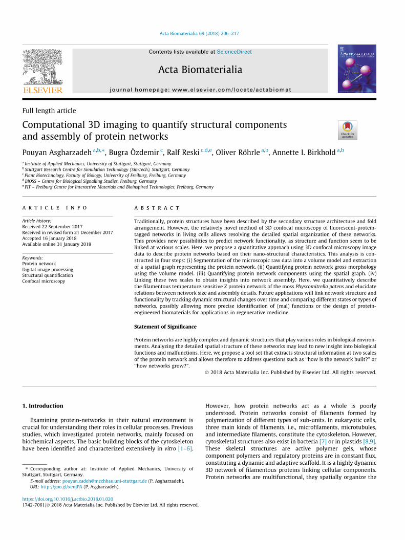
Fig. 1. (a) Confocal microscopy images of several fluorescent-labeled FtsZ proteins inside chloroplasts of one Physcomitrella patens cell (voxel size: 101 nm in x� ydimensions and 300 nm in z dimension). (b) Raw 3D image of one protein network of FtsZ (voxel size: 21 nm in x� y dimensions and 240 nm in z dimension). (c) Segmentednetwork. (d) Wrapped hull determined from segmented image. Images in (c) and (d) have the same voxel size as (b).

208 P. Asgharzadeh et al. / Acta Biomaterialia 69 (2018) 206–217

deconvolved using Huygens Professional software (Scientific Vol-ume Imaging B.V) based on the theoretical point spread functionand the Classical Maximum Likelihood Estimation (CMLE)algorithm.

2.3. Image processing

To extract quantitative measures of the network structure from3D microscopic images we designed an image processing frame-work containing several steps. First, raw images (Fig. 1b) are seg-mented using a semi-automatic iterative approach (Fig. 1c);second, a 3D geometric volume model is created and its overallshape is analyzed (Fig. 1d). Third, it is converted into a spatialgraph, which allows to extract the network topology (nodes, con-nections, segments; Fig. 2). From these two representatives of thenetwork, descriptors of the overall shape of the network and

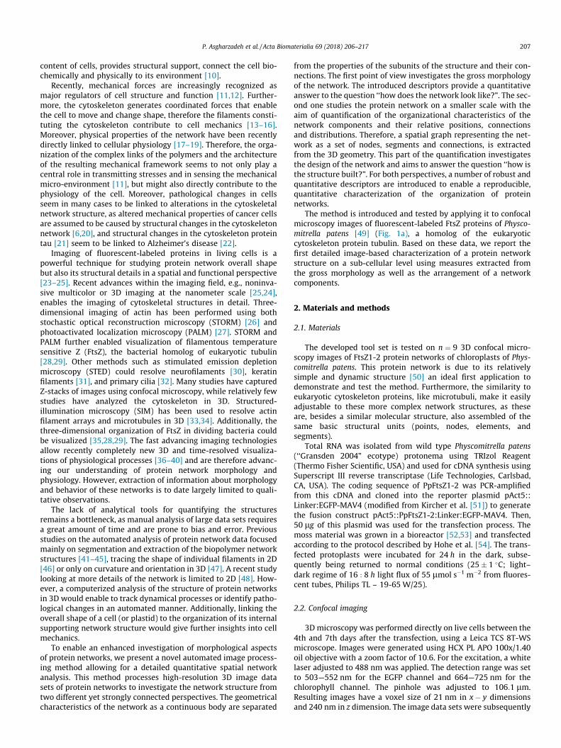
Fig. 2. Transformation of the Segmented Image into a Spatial Graph. (a) Segmentedimage of a protein network of FtsZ. (b) The spatial graph extracted of the segmentedimage. Nodes are shown in light green and segments are shown in a yellow ! redcolor code with red representing thicker segments. (c) Zoomed in part of thenetwork showing individual points in white. (For interpretation of the references tocolour in this figure legend, the reader is referred to the web version of this article.)

descriptors of the detailed morphology of the network and thesub-structure are determined.

2.3.1. Segmentation to extract networkThe image is segmented using an adaptive local threshold algo-

rithm based on median value in each 3D window (window size =10⁄10⁄10 voxels and constant value = 10). Next, the remaining fil-ament discontinuities inside the network are manually corrected.Segmentation was performed in FEI Amira 6.2.0 (Thermo FisherScientific, USA).

2.3.2. Extraction of network gross morphologyThe gross morphology of the network is studied as a whole.

Therefore, a solid outer surface is defined for the segmented imageto find the volume enclosing the network. First, for each slice of the3D image stack the convex hull, represented by the smallest con-vex set containing all the voxels, is determined. The combinationof all convex hulls of all slices forms a wrapped hull around thewhole network (FEI Amira 6.2.0 (Thermo Fisher Scientific, USA)).Second, instead of the detailed network, the solid outer surfaceof the network represented by its wrapped hull is analyzed. Ashape matrix describing the shape and the orientation of thewrapped hull of the network structure is calculated, adapted fromthe shape analysis for whole cells and pulmonary systems pre-sented by Mc Creadie et al. [55] and Chandran et al. [56], respec-tively. Therefore, each voxel is represented as XðiÞ ¼ fx; y; zg, withx; y and z as the coordination of the voxel i. Furthermore, for eachvoxel, the displacement vector from the center of mass is definedas MðiÞ ¼ XðiÞ � C, with C as the center of the mass. The shapematrix representing the solid outer surface is built as:

S ¼ 1n

Xni¼1

MxðiÞMxðiÞ MxðiÞMyðiÞ MxðiÞMzðiÞMyðiÞMxðiÞ MyðiÞMyðiÞ MyðiÞMzðiÞMzðiÞMxðiÞ MzðiÞMyðiÞ MzðiÞMzðiÞ

264

375; ð1Þ

with n as the number of voxels in the segmented image. This 3� 3matrix is created for the covariance of the coordinates of all voxelsof the wrapped hull. This part was done in Matlab 2017a (Math-Works, USA).

2.3.3. Calculation of network shape descriptorsAll the following steps are performed using an inhouse Matlab

code (Matlab 2017a, MathWorks, USA). Shape descriptors aredefined and calculated based on the segmented image, its wrappedhull and its shape matrix to characterize the spatial extensions ofthe network as a whole:

1. The network volume is defined as

VPN ¼ nPN � dx � dy � dz ð2Þ

P. Asgharzadeh et al. / Acta Biomaterialia 69 (2018) 206–217 209

and calculated from the number of the foreground voxels (nPN) ofthe segmented image. dx; dy and dz are the extensions of the vox-els in x, y and z directions, respectively.

2. The enclosed volume of the network is computed as

VEN ¼ nEN � dx � dy � dz ð3Þand defined as the space occupied by the network and the emptyspace inside the network. It is determined by counting the num-ber of voxels (nEN) inside the wrapped hull.

3. The network volume density, qPN , describes how densely thevolume inside the network (wrapped hull) is occupied by mate-rial. It is determined as the ratio of the enclosed volume and thenetwork volume

qPN ¼ VPN

VEN: ð4Þ

4. The greatest and smallest diameters of the network, dmaxPN and

dminPN ; respectively, are calculated by scaling the respective eigen-

values of the shape matrix, as introduced for whole cell analysis[55]:

dmaxPN ¼ 2

ffiffiffi5

pks;3;

dminPN ¼ 2

ffiffiffi5

pks;1; ð5Þ

where, ks;3 > ks;2 > ks;1 are the eigenvalues of the diagonalizedresulted symmetric shape matrix, which define the ellipsoidaxes of the wrapped hull.Spatial anisotropies in the network shape are quantified by ana-lyzing the ratios between the diameters/eigenvalues and theparameters stretch and oblateness of the network are intro-duced. These descriptors have been previously presented to ana-lyze the shape of bone cells [57].

5. The stretch of the network, StPN , describes the elongation of theprotein network and is calculated as the difference between thelargest (ks;3) and smallest eigenvalue (ks;1) of the shape matrix,normalized by the largest one:

StPN ¼ ks;3 � ks;1ks;3

: ð6Þ

StPN 2 ½0;1�; 0 corresponds to a perfect sphere and 1 refers to aninfinitely stretched object (cylinder).

6. The oblateness of the network, ObPN , is defined as

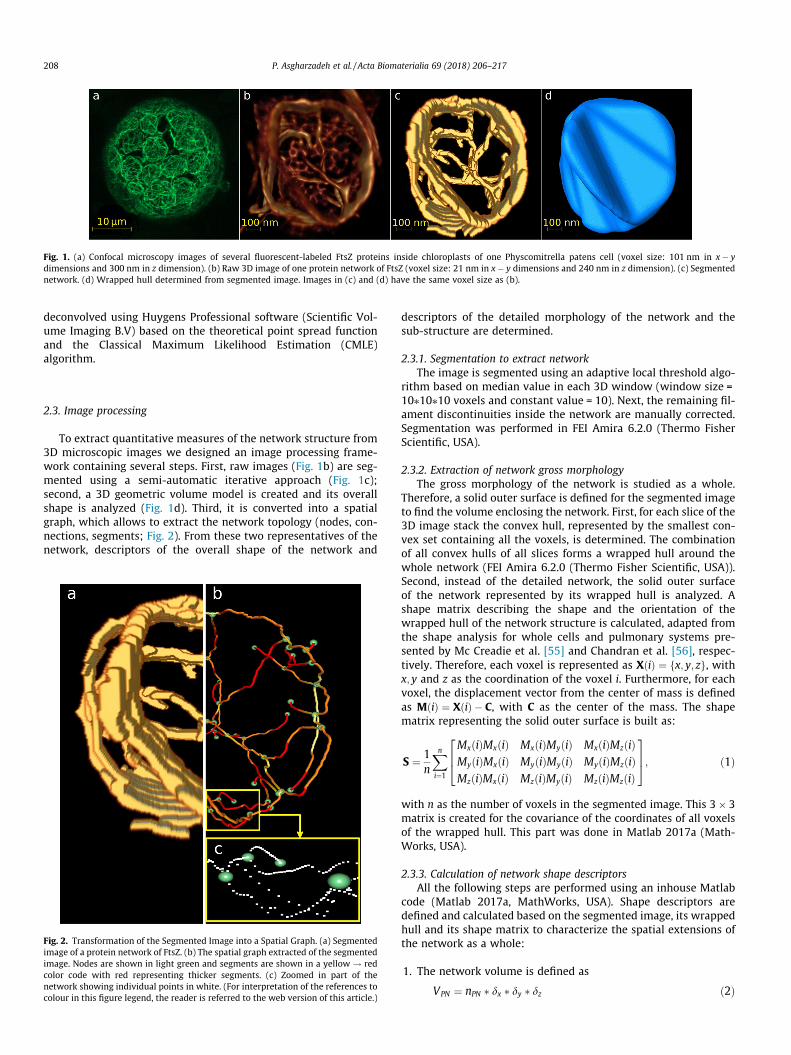
Fig. 3. Node descriptors. A spatial graph of a protein network of FtsZ represented bynodes (light green) and segments (which are shown in a yellow ! red color codewith red representing thicker segments.). The red dot indicates the position of thecenter of the gravity of the network. The green arrows show the distances betweentwo connected nodes ðdninj ). The blue arrow indicates the distance of a node to thecenter of gravity dnic . The purple line represent the distance of a node to the surfaceof the network dnis . (For interpretation of the references to colour in this figurelegend, the reader is referred to the web version of this article.)

ObPN ¼ 2 � ks;2 � ks;1ks;3 � ks;1

� 1: ð7Þ

ObPN 2 ½�1;1� classifies rod-like and plate-like structures. If thesecond eigenvalue, k2, is closer to the greatest eigenvalue, k3,then the object is considered to be elongated. An oblatenessvalue equal to �1 indicates a perfect rod and a value of 1 a per-fect plate.

2.3.4. Extraction of a spatial graphTo extract information about the network micro-structure, a

transformation to a numerical representative, defined by points,nodes and segments, representing the different elements of thecomplex network, is performed. This transformation process isbuilt upon the concept of tensegrity structures and spatial trussesintroduced by Ingber et al. for the analysis of cytoskeleton andendothelial mechanotransmission [58,59], adapted from an imple-mentation for extracting network geometry of collagen gels byStein et al. [60]. First the edge voxels are determined using thegradient rf of the image f:

rf ¼ @f@x

ex þ @f@y

ey þ @f@z

ez; ð8Þ

where ex; ey and ez are unit vectors forming an orthogonal basis.Second, the centerlines of the filamentous structures are identified(Fig. 2b) based on calculating a distance map of all voxels from thenearest edge voxel. Afterwards, points are placed at the centerlineof each structure entity [61]. A point is placed at any part of thestructure at which a change in either the thickness or the directionof the filament occurs (Fig. 2c). Hence, the distances between thepoints are based on the resolution of the original image and com-plexity of the structure. Last, all consecutive points are connectedby elements. As a result, the following components are determinedto numerically represent the network (Fig. 2b, c):

Points: The basic entity of the extracted spatial graph. Points areconnected through elements.

Elements: Connection between two points. Nodes: Points that are connected to more than two other points. Segments: A sequence of elements starting from one node andending at another node.

Connection: Intersection of segments.

For further analysis, the following information is extracted ateach point: an identification (ID) number, coordination, thicknessof the filament at that point and the IDs of the neighboring pointsto which this point is connected to. The network extraction stepswere performed in FEI Amira (Thermo Fisher Scientific, USA).

2.3.5. Calculation of network element descriptorsThe segmented image and the information from the spatial

graph are further analyzed together to quantify details of the net-work structure details (inhouse Matlab code (Matlab 2017a, Math-Works, USA)):

Node descriptors (Fig. 3):1. Number of nodes in the network, Nn.

210 P. Asgharzadeh et al. / Acta Biomaterialia 69 (2018) 206–217

2. Node thickness thni is determined by the diameter of the fila-ment at the location of the node, ni.

3. Node density, qn, is defined by

qn ¼ Nn

VEN; ð9Þ

and determined by the number of nodes normalized to the vol-ume enclosed by the network ð1=lm3Þ. It has to be taken inmind, that this in not the same as the network volume density.

4. Node-to-node distance, dninj ,

dninj ¼ kni � njk2 ¼ ðffiffiffiffiffiffiffiffiffiffiffiffiffiffiffiffiffiffiffiffiffiffiffiffiffiffiffiffiffiffiffiffiffiffiffiffiffiffiffiffiffiffiffiffiffiffiffiffiffiffiffiffiffiffiffiffiffiffiffiffiffiffiffiffiffiffiffiffiðxi � xjÞ2 þ ðyi � yjÞ2 þ ðzi � zjÞ2

q;

ð10Þis calculated as the Euclidean distance between two neighbor-ing nodes, ni and nj, with coordinates xi; yi and zi, and xj; yj andzj, respectively.

5. The node-to-surface distance, dnis, represents the closest dis-tance of the node ni to the surface of the network. This ele-ment descriptor represents the local distribution of thenodes within the network.

6. Compactness of the network, CPN , is defined by

CPN ¼ dnc � dns

dnc; with dnc ¼ 1

n

Xn

i¼1

dnic; and dns ¼ 1n

Xni¼1

dnis;

ð11Þwhere, dnic , the node-to-center distance, is the distance of eachnode to the center of gravity of all nodes. It is calculatedaccording to node-to-surface distance (Eq. (10)) by replacingthe second node with the center of gravity. We define the com-pactness of the network as the difference between the meandistance to the center of gravity and the mean distance tothe network surface of all nodes, normalized by the mean dis-tance to the center of gravity; CPN 2 ½0;1�. For CPN ¼ 1, all thenodes are placed at the surface of the network. In contrary,CPN converges toward 0 if all nodes are placed near the centerof gravity.

7. Node-to-surface to node-to-center distance ratio, dnis=dnic ,provides information on whether the node is located closerto the surface of the network or to the center of gravity.

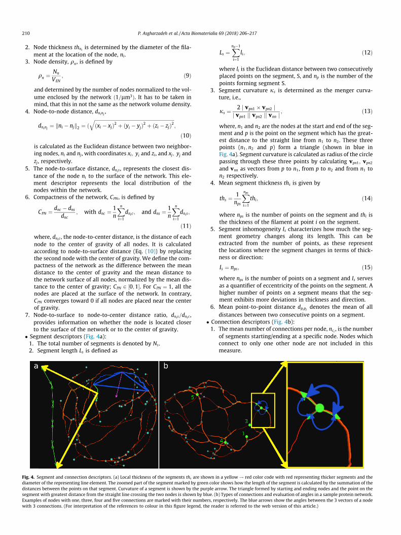
Segment descriptors (Fig. 4a):1. The total number of segments is denoted by Ns.2. Segment length Ls is defined as

Fig. 4. Segment and connection descriptors. (a) Local thickness of the segments ths are sdiameter of the representing line element. The zoomed part of the segment marked by gredistances between the points on that segment. Curvature of a segment is shown by the psegment with greatest distance from the straight line crossing the two nodes is shown byExamples of nodes with one, three, four and five connections are marked with their numwith 3 connections. (For interpretation of the references to colour in this figure legend,

Ls ¼Xnp�1

i¼1

li; ð12Þ

where li is the Euclidean distance between two consecutivelyplaced points on the segment, S, and np is the number of thepoints forming segment S.

3. Segment curvature js is determined as the menger curva-ture, i.e.,

js ¼ 2 j vpn1 � vpn2 jj vpn1 jj vpn2 jj vnn j ; ð13Þ

where, n1 and n2 are the nodes at the start and end of the seg-ment and p is the point on the segment which has the great-est distance to the straight line from n1 to n2. These threepoints (n1;n2 and p) form a triangle (shown in blue inFig. 4a). Segment curvature is calculated as radius of the circlepassing through these three points by calculating vpn1; vpn2

and vnn as vectors from p to n1, from p to n2 and from n1 ton2 respectively.

4. Mean segment thickness ths is given by

ths ¼ 1nps

Xnpsi¼1

thi; ð14Þ

where nps is the number of points on the segment and thi isthe thickness of the filament at point i on the segment.

5. Segment inhomogeneity Is characterizes how much the seg-ment geometry changes along its length. This can beextracted from the number of points, as these representthe locations where the segment changes in terms of thick-ness or direction:

Is ¼ nps; ð15Þwhere nps is the number of points on a segment and Is servesas a quantifier of eccentricity of the points on the segment. Ahigher number of points on a segment means that the seg-ment exhibits more deviations in thickness and direction.

6. Mean point-to-point distance dpipj denotes the mean of alldistances between two consecutive points on a segment.

Connection descriptors (Fig. 4b):1. The mean number of connections per node, nci , is the number

of segments starting/ending at a specific node. Nodes whichconnect to only one other node are not included in thismeasure.

hown in a yellow ! red color code with red representing thicker segments and theen color shows how the length of the segment is calculated by the summation of theurple arrow. The triangle formed by starting and ending nodes and the point on theblue. (b) Types of connections and evaluation of angles in a sample protein network.bers, respectively. The blue arrows show the angles between the 3 vectors of a nodethe reader is referred to the web version of this article.)

P. Asgharzadeh et al. / Acta Biomaterialia 69 (2018) 206–217 211

2. Open nodes, noe, denotes the percentage of all nodes in thenetwork that are only connected to one other node, i.e.,nodes that are end nodes.

3. The mean angles between the segments at a connection, �hci isdefined as

Fig. 5.segmenautomadistancnumberHausdoR2 ¼ 0:2

�hci ¼1n

Xnj¼1

hj; ð16Þ

with,

hj ¼ arccosvk � vl

j vk jj vl j ; k; l 2 f1; . . . ;ng; ð17Þ

where �hci is the average of angles (hj) between segmentsmeeting in one connection. Angle hj is evaluated by calculat-ing the angle between the vectors vk and vl, which start fromnode ni located at the center of the connection and go to thefirst point on each of the meeting segments. Hence, for a nodewith three connections, three different angles for each pair ofoutgoing segments (three pairs) are calculated as hj, there-fore, �hci is the mean value of these 3 calculated angles(Fig. 4b, indicated in blue).

Descriptors are calculated using an inhouse Matlab code (Mat-lab 2017a, MathWorks, USA).

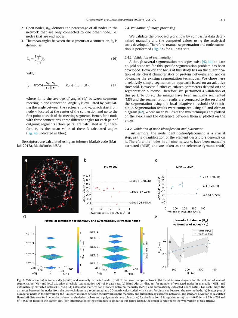
Validation. (a) Automatically (white) and manually extracted nodes (red) of ttation (MS) and local adaptive threshold segmentation (AS) of 9 data sets. (ctically extracted networks (ANE). (d) Calculated matrices for distances betweees between the nodes from the two techniques are represented as a 2D matrix cof nodes in the network vs. the Hausdorff distance between the networks in the mrff distances for 9 networks is shown as shaded error bars and a polynomial curve9) is fitted to the scatter plot. (For interpretation of the references to colour in

2.4. Validation of image processing

We validate the proposed work flow by comparing data deter-mined manually and the computed values using the analyticaltools developed. Therefore, manual segmentation and node extrac-tion is performed (Fig. 5a) for all data sets.

2.4.1. Validation of segmentationAlthough several segmentation strategies exist [42,44], to date

no gold standard for this specific segmentation problem has beendeveloped. However, the focus of this study lies on the quantifica-tion of structural characteristics of protein networks and not onadvancing the existing segmentation techniques. We chose herea relatively simple segmentation approach based on an adaptivethreshold. However, further calculated parameters depend on thesegmentation outcome. Therefore, we performed a validation ofthis part. To do so, the images have been manually segmented(MS) and the segmentation results are compared to the results ofthe segmentation using the local adaptive threshold (AS) tech-nique. Segmentation results were compared using a Bland Altmandiagram [62], where mean values of the two techniques are plottedon the x-axis and the difference between them is plotted on they-axis.

2.4.2. Validation of node identification and placementFurthermore, the node identification/placement is a crucial

step, as the quantification of the element descriptors depends onit. Therefore, the nodes in all nine networks have been manuallyextracted (MNE) and are taken as the reference (ground truth)

he same sample network. (b) Bland Altman diagram for the volume of manual) Bland Altman diagram for number of extracted nodes in manually (MNE) andn manually (MNE) and automatically extracted nodes (ANE). For each image theolor-coded with values for distances between the two methods. (e) Scatter plot ofanually and automatically extracted networks. The standard deviation of calculated(blue curve) for the data from 9 image data sets (f ðxÞ ¼ �0:001x2 þ 1:33xþ 768 andthis figure legend, the reader is referred to the web version of this article.)

212 P. Asgharzadeh et al. / Acta Biomaterialia 69 (2018) 206–217

for the node placement step (ANE) of the proposed method(Fig. 5a). All further descriptors are directly derived from thesetwo intermediate steps and are therefore not validated here.

First, the number of extracted nodes in each network is deter-mined. Second, we calculated the vertex error

EV ¼ 12 j Nm j

Xpm2Nm

minpa2Na

jj pm � pa jj þ1

2 j Na jXpa2Na

minpm2Nm

j

j pa � pm jj; ð18Þand Hausdorff distance

HD ¼ max maxpm2Nm

minpa2Na

jj pa � pm jj;maxpa2Na

minpm2Nm

jj pm � pa jj� �

; ð19Þ

[63] between the nodes in the manually and automaticallyextracted networks. Nm and Na denote manually and automaticallyextracted networks, pm and pa are the nodes in the manually andautomatically extracted networks, respectively. Third, the distancesbetween the nodes in the manually and the automatically extractednetworks have been calculated and a color-code is assigned. Thevalue of the cell ðm;nÞ represents the distance between the nthmanually extracted and mth automatically extracted node. Last,the relation between the Hausdorff distance and number of thenodes in the network, which is directly related to the size and com-plexity of the network, has been analyzed.

2.5. Statistical analysis

To identify relationships between calculated descriptors regres-sion analysis were performed and Pearson correlation coefficients

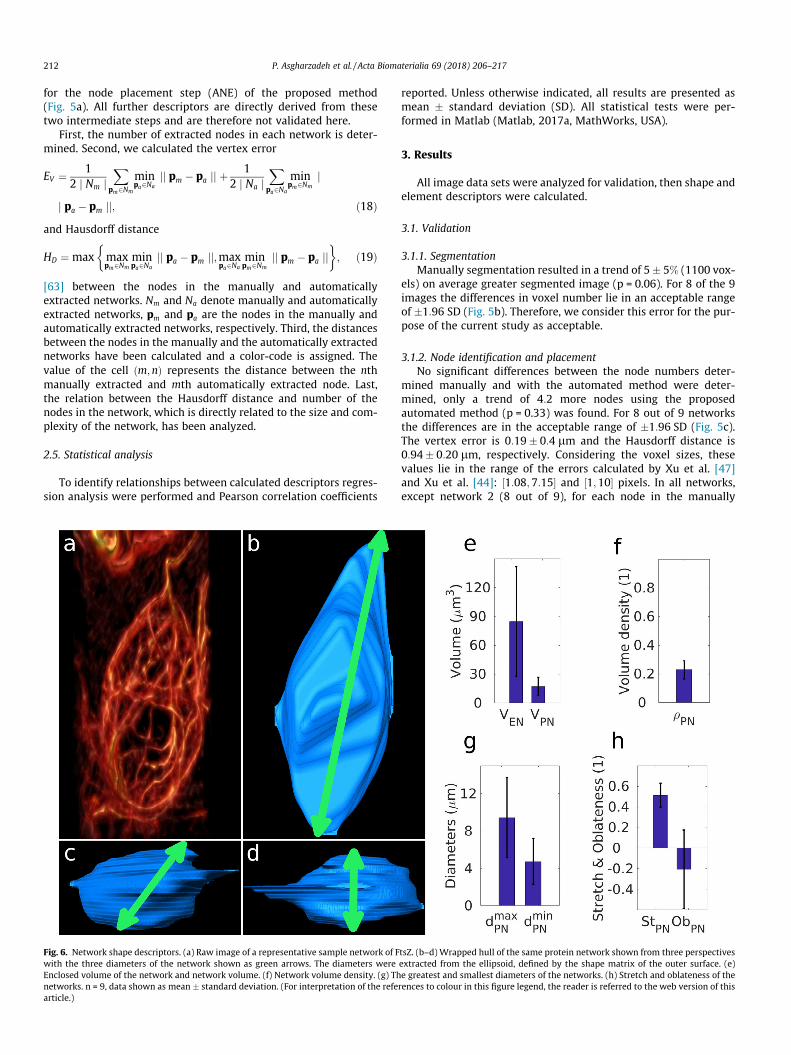
Fig. 6. Network shape descriptors. (a) Raw image of a representative sample network of Fwith the three diameters of the network shown as green arrows. The diameters wereEnclosed volume of the network and network volume. (f) Network volume density. (g) Thnetworks. n = 9, data shown as mean � standard deviation. (For interpretation of the refearticle.)

reported. Unless otherwise indicated, all results are presented asmean � standard deviation (SD). All statistical tests were per-formed in Matlab (Matlab, 2017a, MathWorks, USA).

3. Results

All image data sets were analyzed for validation, then shape andelement descriptors were calculated.

3.1. Validation

3.1.1. SegmentationManually segmentation resulted in a trend of 5� 5% (1100 vox-

els) on average greater segmented image (p = 0.06). For 8 of the 9images the differences in voxel number lie in an acceptable rangeof �1:96 SD (Fig. 5b). Therefore, we consider this error for the pur-pose of the current study as acceptable.

3.1.2. Node identification and placementNo significant differences between the node numbers deter-

mined manually and with the automated method were deter-mined, only a trend of 4:2 more nodes using the proposedautomated method (p = 0.33) was found. For 8 out of 9 networksthe differences are in the acceptable range of �1:96 SD (Fig. 5c).The vertex error is 0:19� 0:4 lm and the Hausdorff distance is0:94� 0:20 lm, respectively. Considering the voxel sizes, thesevalues lie in the range of the errors calculated by Xu et al. [47]and Xu et al. [44]: ½1:08;7:15� and ½1;10� pixels. In all networks,except network 2 (8 out of 9), for each node in the manually

tsZ. (b–d) Wrapped hull of the same protein network shown from three perspectivesextracted from the ellipsoid, defined by the shape matrix of the outer surface. (e)e greatest and smallest diameters of the networks. (h) Stretch and oblateness of therences to colour in this figure legend, the reader is referred to the web version of this

Fig. 7. Evaluated element descriptors for nodes. (a) Example of a FtsZ protein network with relatively low node number and (b) the corresponding spatial graph withemphasized nodes in green. (c) Example of a FtsZ protein network with relatively high node number and (d) the corresponding spatial graph with emphasized nodes in green.In the spatial graph the segments are shown in a yellow! red color code with red representing thicker segments.(e) Normalized cumulative frequency of the node-to-surfacedistances of the networks. Each line represents one image. (f) Normalized cumulative frequency of the node-to-node distances in networks. Each line represents one image.(g) Normalized cumulative frequency of the node-to-center distances in networks. Each line represents one image. (h) Normalized cumulative frequency of the node-to-surface to node-to-center distances ratio in networks. Each line represents one image. (For interpretation of the references to colour in this figure legend, the reader is referredto the web version of this article.)

Table 1Element Descriptors of FtsZ (n ¼ 9). All descriptors are presented as mean � standarddeviation, unless stated otherwise.

Descriptor Value

Number of nodes 199 ± 130Node density 2.52 ± 0.63 node/lm3

Compactness 0.75 ± 0.10Node thickness 50 ± 10 nmNumber of segments 259 ± 168Mean segment thickness 20 ± 10 nmMean point-to-point distance 55 ± 10 nmSegment inhomogeneity 20.4 ± 3.64Number of connections per node 3.11 ± 0.04Most observed number of connections 3 and 4Open nodes 8.79 ± 2.38%

P. Asgharzadeh et al. / Acta Biomaterialia 69 (2018) 206–217 213

extracted network, there exists a node in the automaticallyextracted network within a distance of 2 lm (dark blue color;Fig. 5d)). This confirms the acceptable error for the method’s abilityto place nodes. When the number of nodes increases, the Hausdorffdistance tends to merge towards a value less than 1:3 lm, wherethe second derivative of the second order polynomial curve(f ðxÞ ¼ �0:001x2 þ 1:33xþ 768 and R2 ¼ 0:29) fitted to the scat-tered diagram is �0:002 (Fig. 5e). We assume to have a similarHausdorff distance for higher node numbers, which would allowapplying this method to more complex protein networks, such ascytoskeletal protein networks. Considering the image resolutionand overall size of the networks, the Hausdorff and vertex errorvalues can be considered small enough to allow a quantitativeanalysis of the images. However, when interpreting the resultsthey have to be taken into account.

3.2. What is the shape of the network?

Primary gross morphology features of the network as a wholewere evaluated (Fig. 6). A wrapped hull of a network and its threediameters are shown for a sample network in Fig. 6a–d. The

enclosed volume of the network VEN showed a great variation(84:9� 56:9 lm3), whereas the network volume VPN

(17:2� 9:74 lm3) and network volume density qPN (0:23� 0:06)displayed smaller variations. The greatest and smallest diameters

of the network, dmaxPN and dmin

PN , are 9:45� 4:32 lm and4:75� 2:47 lm. Furthermore, the stretch of the network StPNshowed a smaller variation (0:51� 0:11) than the oblateness ofthe network ObPN (�0:20� 0:38; Fig. 6e–h).

3.3. Nodes – basics of the network

Individual nodes are identified and analyzed. For the investi-gated networks a wide range of number of nodes was found(199� 130; Fig. 7a–d), whereas the size of individual nodes (nodethickness 50� 10 nm) and normalized parameters like the com-pactness and node density were more homogeneous (0:75� 0:10and 2:52� 0:63 node=lm3, respectively). Additionally, the relativepositions of the nodes in the network give further insight into theconstruction of the network (Table 1). Connected nodes have beenidentified and the average node-to-node distance (0:57� 0:05 lm)was determined. Analyzing the distribution of distances showed,that 90% of all nodes are closer than 0:93 lm to their closest neigh-bor. In contrast, nodes have only an average distance of0:50� 0:20 lm to the surface of the network, with 90% of thembeing closer than 1:16 lm to the surface (Fig. 7e, f). Moreover,for values of node-to-center distance a considerable variationbetween the networks was observed (Fig. 7g) whereas the node-to-surface to node-to-center distance ratio (Fig. 7h) showed lessvariation in different networks (2:20� 0:74 lm and 0:28� 0:09,respectively).

3.4. Segments – filamentous nature of the network

The analyzed networks had 258� 168 segments with a meanthickness of 25� 5 nm and a mean length of 0:78� 0:07 lm. To

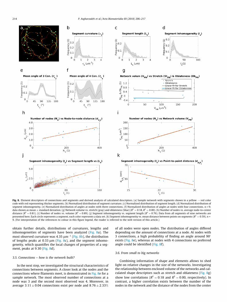
Fig. 8. Element descriptors of connections and segments and derived analysis of calculated descriptors. (a) Sample network with segments shown in a yellow ! red colorcode with red representing thicker segments. (b) Normalized distribution of segment curvature. (c) Normalized distribution of segment length. (d) Normalized distribution ofsegment inhomogeneity. (e) Normalized distribution of angles at nodes with three connections. (f) Normalized distribution of angles at nodes with four connections. n = 9;data shown as mean � standard deviation. (g) Network volume vs. stretch (gray) and oblateness (blue) (R2 ¼ 0:18, R2 ¼ 0:00). (h) Number of nodes vs. average node-to-centerdistance (R2 ¼ 0:81). (i) Number of nodes vs. volume (R2 ¼ 0:89). (j) Segment inhomogeneity vs. segment length (R2 ¼ 0:76). Data from all segments of nine networks arepresented here. Each circle represents a segment, each color represents a data set. (k) Segment inhomogeneity vs. mean distance between points on segments (R2 ¼ 0:59). n =9. (For interpretation of the references to colour in this figure legend, the reader is referred to the web version of this article.)

214 P. Asgharzadeh et al. / Acta Biomaterialia 69 (2018) 206–217

obtain further details, distributions of curvatures, lengths andinhomogeneities of segments have been analyzed (Fig. 8a). Themost observed curvature was 4:35 lm�1 (Fig. 8b), the distributionof lengths peaks at 0:33 lm (Fig. 8c), and the segment inhomo-geneity, which quantifies the local changes of properties of a seg-ment, peaks at 9:30 (Fig. 8d).

3.5. Connections – how is the network built?

In the next step, we investigated the structural characteristics ofconnections between segments. A closer look at the nodes and theconnections where filaments meet, is demonstrated in Fig. 8e for asample network. The most observed number of connections at anode was 3 and the second most observed was 4. Moreover, inaverage 3:11� 0:04 connections exist per node and 8:76� 2:33%

of all nodes were open nodes. The distribution of angles differeddepending on the amount of connections at a node. At nodes with3 connections, a high probability of finding an angle around 90�

exists (Fig. 8e), whereas at nodes with 4 connections no preferredangle could be identified (Fig. 8f).

3.6. From small to big networks

Combining information of shape and elements allows to shedlight on relative changes in the size of the networks. Investigatingthe relationship between enclosed volume of the networks and cal-culated shape descriptors such as stretch and oblateness (Fig. 8g)show low correlations (R2 ¼ 0:18 and R2 ¼ 0:00, respectively). Incontrast, a higher correlation exists between the number of thenodes in the network and the distance of the nodes from the center

P. Asgharzadeh et al. / Acta Biomaterialia 69 (2018) 206–217 215

(Fig. 8h), showing that a higher number of nodes results in nodesbeing located further away from the center of mass (R2 ¼ 0:81).The size of the network also correlates strongly with the numberof nodes in the network (R2 ¼ 0:89; Fig. 8i). When the network vol-ume is twice as great (e.g. 100 ! 200 lm3), also the number ofnodes is approximately doubled; but with increasing network sizethe node placement is not homogeneously propagated, as the aver-age distance of the nodes from the center increased at the same timeby a factor of 1:5. Furthermore, the combination of node-to-surfaceand node-to-center distance measurements (Fig. 7e and g) suggeststhat the average value of compactness for the data is closer to 1 thanto 0. This is confirmed by calculating the average compactness (cf.compactness in Table 1). Besides these global relationships betweenthe size of networks and shape and element descriptors, segmentgrowth can be analyzed on a local scale. On one hand, with longersegments the segment inhomogeneity increases (Fig. 8j). On theother hand, the increase in segment inhomogeneity results in smal-ler distances between the points within segments (Fig. 8k).

4. Discussion

To date, analysis of protein network structures as basis forcytoskeletal behaviour assessment is mainly qualitative. However,with current advanced microscopy and labeling techniques, local-ized cytoskeletal behavior can be imaged with great detail, allow-ing for a quantitative network analysis. Here, we analyzedpossibilities to quantitatively describe the structure of protein net-works and provided a tool set, which contributes to such a quanti-tative network analysis. To show the capabilities of this tool set, itwas validated using confocal microscopy images of FtsZ.

The observed variations in calculated shape descriptors(Fig. 6e–g) of FtsZ show that although there exist great variationsbetween the sizes of the analyzed networks, the network volumedensity shows lower deviation from the mean value. This conveysthat in networks from small to big, the network volume densitydoes not change remarkably. In cases of ellipsoidal-like networkshapes, like for FtsZ [64], morphological characteristics such asdiameters of the network and relationships between these calcu-lated descriptors can be analyzed (Fig. 6g). Therefore, stretch andoblateness of the network are identified (Fig. 6h). The stretch val-ues indicate a deviation of the shape of the networks from a sphereto a more stretched geometry while the oblateness measurementsconvey the tendency toward more rod-shaped networks. However,the greater variation in oblateness shows that stretch is, for theanalyzed data sets, a better measure of the shape of the network.

Analysis of the element components of protein network allowsdetailed quantification of the subunits of the network. This analysisenables to quantitatively describe the characteristics of structuralunits of the network: nodes, connections and segments. Node-to-surface distances are relatively similar for all analyzed FtsZ net-works, the distance of the nodes from the center of mass shows agreat variation between networks. Quantifying relative positionsof the nodes is in future applications useful in terms of studyingdynamic settings of networks and to identify changes that occurin the network as a result of external stimuli on the structure ofthe network or internally motivated changes.

The shape measures allow to relate changes of the protein net-work size and shape to alterations of the plastid, or cells in the caseof other protein networks, morphology, which will allow in futureapplications to relate protein network alterations to cellular pro-cesses. For example, during cell division the cell, and accordinglythe cytoskeleton, elongates from its initial form to a morestretched shape [65]. Furthermore, in cancerous cells, cytoskeletonprotein transformations lead to changes in mechanical propertiesof the cancer cells in contraction, stretchability and deformability

[66]. For example, epithelial-to-mesenchymal transition in col-orectal cancer cells results in transformation of the cytoskeletoninto a spindle-shape losing their polarity [67]. Moreover, propaga-tion of tau filaments from cell to cell in Tauopathic diseases havebeen shown to result in protein network changes [68,69]. All theseprocess could be investigated quantitatively with the here intro-duced shape descriptors in future studies.

Analysis of segments have been previously shown by Smith et al.[42] and Alioscha et al. [46] to link actin filaments fragments in seg-mented images and by Stein et al. [60] for extracting network geom-etry of collagen gels. Moreover, Xu et al. [47] analyzed differentfilamentous protein networks. To obtain a complete protein net-work analysis method, we included these entities in our shape andelement analysis and adapted the calculation of these to our struc-tural quantificationmethod. Analyzing the segments of the networkdoes not only shed light on the local attributes of the filaments, butalso allows to draw further conclusions on the mechanical proper-ties of the networks, as e.g. the curvature of the segments allowsto quantifymechanical forces on the filament [70] or effects of shearstress [46]. Segment length can be used to track changes that willtransform the architecture of the network in a more fundamentalway. The angles between the segments meeting in one connectiongive insight into the shape of individual sub-compartments of thenetwork. Also, it might be applicable to track the effects of externalstimuli on the network such as shear forces, which elongate the fil-aments and change the angles between them in the network [46]. Inthe here analyzed networks a great variation of angles between con-nections was observed, which might be caused by such externalstimuli. Therefore, tracking structural descriptors might enhancethe understanding of the dynamic setup of network structures, byallowing to monitor and quantify changes occurring in various pro-cesses that alter the shape of the network.

Linking shape and element descriptors gives insights into howthe shape of protein networks changes during different processeswithoutbeing transformed intoamore stretchedorplate-like shape.More nodes resulted in nodes being located further away from thecenter of mass. This shows that FtsZ networks might grow in sizeby adding nodes in radial direction form the center of gravity closeto the surface, consequently resulting in networks with higher vol-ume. Moreover, the relation between the size of the network andnumber of nodes in the network conveys the possibility of a pre-ferred approach of the network to grow. The network seems to growin volume by adding more nodes to the existing network instead ofpreserving the nodes and adding more connections to the existingnodes. Finally, we found, that there exists a direct correlationbetween the length of the segments and the inhomogeneity of thesegments.

Our study has several limitations. We study protein networks inliving cells. Therefore, assembly and disassembly is a dynamic pro-cess that generates inhomogeneities. Furthermore, the spatial res-olution, especially in z-resolution, does not allow to resolve allsmall structures in the images and therefore, impacts the resultsas well. However, the fast advancing field of microscopy technol-ogy will allow to overcome this limitation in future applications.A main limitation of our method is the segmentation, as it is inmost imaging studies. Global threshold algorithms such as theOtsu-Algorithm [71] are commonly used to extract the geometryof filaments [48]. However, the presence of imaging-specific arti-facts, like filament discontinuities, high signal-to-noise ratioresulting from presence of overexposed pixels and dynamics ofthe network, decrease the efficiency of global algorithms. There-fore, we used an adaptive threshold algorithm, which accountsfor intensity variations. However, variations in the input imagequality effects the segmentation outcomes, therefore a manual cor-rection is applied, which introduces user bias. An enhanced seg-mentation in future studies could include linkage of filament

216 P. Asgharzadeh et al. / Acta Biomaterialia 69 (2018) 206–217

fragments, as previously presented for microtubule network archi-tecture phenotypes in fibroblasts [48]. Therefore, care must betaken in the analysis to avoid systematic errors. It should also betaken in mind, that the approach used here might not be directlyapplicable to other network shapes, as we assume an ellipsoidalshape, approximated by 2 vectors and 3 scalar quantities. For other(more complex) shapes, different shape models have to be used.

5. Conclusion and outlook

The regulations of individual proteins and their functions havebeen investigated in detail in the past [72]. Here, we presented amethod to quantify the structure of protein networks. Proteinsforming networks in biological environments are many copies ofa few key pieces, which can be assembled into a wide range ofstructures depending on how the pieces are assembled. Themethod presented here provides a quantitative tool to investigatethis meso-scale of the assembly. This analysis can potentially beused to study temporal evolution of the network by batch process-ing consecutive frames of a time lapsed life image sequence. Ana-lyzing the structure of the network in each frame and trackingchanges of structural features might allow relating internal andexternal stimuli to the modifications of the structure by utilizinga network-based simulation model and might contribute to deter-mining functionality of the network. Here, we analyzed the FtsZprotein network structure and revealed aspects of this internalorganization. In the future, the developed method can be appliedto compare networks to identify relationships between structuraland functional differences. Furthermore, more complex networkssuch as cytoskeletons [73,74] can be analyzed, as these are builtof the same basic structural units. This analysis would facilitateunderstanding the links between the interactions of the individualunits of the network and the large-scale cellular behaviors depend-ing on them [13]. Linking network structure and functionality bytracking dynamic structural changes over time and comparing dif-ferent states or types of networks, may allow to more preciselyidentify (mal) functions or design protein-engineered biomaterialsfor applications in regenerative medicine.

Contributions

Study concept and design: PA, OR, AB, RR. Molecular biology,imaging and deconvolution: BO. Contributing software: PA. Analy-sis of data: PA. Interpretation of data: PA, AB. Writing manuscript:PA. Critical revision: All authors. The developed codes in Matlaband the work flow in Amira will be provided by the correspondingauthor upon request.

Disclosures

The authors state that they have no conflict of interest.

Acknowledgements

This work has been funded by the German Research Foundation(DFG) as part of the Transregional Collaborative Research Centre(SFB/Transregio) 141 ‘Biological Design and Integrative Structures’,A09 project.

References

[1] F. MacKintosh, J. Käs, P. Janmey, Elasticity of semiflexible biopolymernetworks, Phys. Rev. Lett. 75 (1995) 4425–4428.

[2] M. Gardel, J. Shin, F. MacKintosh, L. Mahadevan, P. Matsudaira, D. Weitz, Elasticbehavior of cross-linked and bundled actin networks, Science 304 (2004)1301–1305.

[3] C. Storm, J.J. Pastore, F. MacKintosh, T. Lubensky, P.A. Jamney, Nonlinearelasticity in biological gels, Nature 435 (2005) 191–194.

[4] G.H. Koenderink, Z. Dogic, F. Nakamura, P.M. Bendix, F.C. MacKintosh, J.H.Hartwig, T.P. Stossel, D.A. Weitz, An active biopolymer network controlled bymolecular motors, Proc. Natl. Acad. Sci. U.S.A. 106 (2009) 15192–15197.

[5] S. Köster, D.A. Weitz, R.D. Goldman, U. Aebi, H. Herrmann, Intermediatefilament mechanics in vitro and in the cell: from coiled coils to filaments, fibersand networks, Curr. Opin. Cell Biol. 32 (2015) 82–91.

[6] K. Mandal, A. Asnacios, B. Goud, J.-B. Manneville, Mapping intracellularmechanics on micropatterned substrates, Proc. Natl. Acad. Sci. U.S.A. 113(2016) E7159–E7168.

[7] J. Errington, Dynamic proteins and a cytoskeleton in bacteria, Nat. Cell Biol. 5(2003) 175–178.

[8] R. Reski, Rings and networks: the amazing complexity of FtsZ in chloroplasts,Trends Plant Sci. 7 (2002) 103–105.

[9] R. Reski, Challenges to our current view on chloroplasts, Biol. Chem. 390 (2009)731–738.

[10] S.F. Badylak, D.O. Freytes, T.W. Gilbert, Extracellular matrix as a biologicalscaffold material: structure and function, Acta Biomater. 5 (2009) 1–13.

[11] P.A. Janmey, C.A. McCulloch, Cell mechanics: integrating cell responses tomechanical stimuli, Ann. Rev. Biomed. Eng. 9 (2007) 1–34.

[12] X. Trepat, L. Deng, S.S. An, D. Navajas, D.J. Tschumperlin, W.T. Gerthoffer, J.P.Butler, J.J. Fredberg, Universal physical responses to stretch in the living cell,Nature 447 (2007) 592–595.

[13] D.A. Fletcher, R.D. Mullins, Cell mechanics and the cytoskeleton, Nature 463(2010) 485–492.

[14] Q. Wen, P.A. Janmey, Polymer physics of the cytoskeleton, Curr. Opin. SolidState Mater. Sci. 15 (2011) 177–182.

[15] M.F. Coughlin, J.J. Fredberg, Changes in cytoskeletal dynamics and nonlinearrheology with metastatic ability in Cancer Cell lines, Phys. Biol. 10 (2013)065001.

[16] F. Huber, A. Boire, M.P. Lopez, G.H. Koenderink, Cytoskeletal crosstalk: whenthree different personalities team up, Curr. Opin. Cell Biol. 32 (2015) 39–47.

[17] B.M. Mulder, M.E. Janson, Biological filaments: self-healing microtubules, Nat.Mater. 14 (2015) 1080–1081.

[18] C. Aumeier, L. Schaedel, J. Gaillard, K. John, L. Blanchoin, M. Théry, Self-repairpromotes microtubule rescue, Nat. Cell Biol. 18 (2016) 1054–1064.

[19] P. Robison, M.A. Caporizzo, H. Ahmadzadeh, A.I. Bogush, C.Y. Chen, K.B.Margulies, V.B. Shenoy, B.L. Prosser, Detyrosinated microtubules buckle andbear load in contracting cardiomyocytes, Science 352 (2016) aaf0659.

[20] M.E. Grady, R.J. Composto, D.M. Eckmann, Cell elasticity with alteredcytoskeletal architectures across multiple cell types, J. Mech. Behav. Biomed.Mater. 61 (2016) 197–207.

[21] T. Arendt, T. Bullmann, Neuronal plasticity in hibernation and the proposedrole of the microtubule-associated protein tau as a master switch regulatingsynaptic gain in neuronal networks, Am. J. Physiol. (Lond.)-Regul. Integr.Compar. Physiol. 305 (2013) R478–R489.

[22] A. Benda, H. Aitken, D.S. Davies, R. Whan, C. Goldsbury, Sted imaging of taufilaments in alzheimer’s disease cortical grey matter, J. Struct. Biol. 195 (2016)345–352.

[23] B. Hein, K.I. Willig, S.W. Hell, Stimulated emission depletion (sted) nanoscopyof a fluorescent protein-labeled organelle inside a living cell, Proc. Natl. Acad.Sci. 105 (2008) 14271–14276.

[24] B. Huang, M. Bates, X. Zhuang, Super resolution fluorescence microscopy,Annu. Rev. Biochem. 78 (2010) 993–1016.

[25] E. Wegel, A. Göhler, B.C. Lagerholm, A. Wainman, S. Uphoff, R. Kaufmann, I.M.Dobbie, ImAging Cellular structures in super-resolution with SIM, STED andLocalisation Microscopy: a practical comparison, Sci. Rep. 6 (2016) 27290.

[26] K. Xu, G. Zhong, X. Zhuang, Actin, spectrin, and associated proteins form aperiodic cytoskeletal structure in axons, Science 339 (2013) 452–456.

[27] F.V. Subach, G.H. Patterson, M. Renz, J. Lippincott-schwartz, V.V. Verkhusha,For two-color super-resolution sptPALM of live cells, Cell (2010) 12651–12656.

[28] ŠBálint, I. Verdeny Vilanova, Á. Sandoval Álvarez, M. Lakadamyali, Correlativelive-cell and superresolution microscopy reveals cargo transport dynamics atmicrotubule intersections, Proc. Natl. Acad. Sci. U.S.A. 110 (2013) 3375–3380.

[29] S.J. Holden, T. Pengo, K.L. Meibom, C. Fernandez Fernandez, J. Collier, S. Manley,High throughput 3D super-resolution microscopy reveals Caulobactercrescentus In Vivo Z-ring organization, Proc. Natl. Acad. Sci. 111 (2014)4566–4571.

[30] N.T. Urban, K.I. Willig, S.W. Hell, U.V. Nägerl, Sted nanoscopy of actin dynamicsin synapses deep inside living brain slices, Biophys. J. 101 (2011) 1277–1284.

[31] G. Vicidomini, G. Moneron, K.Y. Han, V. Westphal, H. Ta, M. Reuss, J.Engelhardt, C. Eggeling, S.W. Hell, Sharper low-power STED nanoscopy bytime gating, Nat. Methods 8 (2011) 571–573.

[32] T.T. Yang, P.J. Hampilos, B. Nathwani, C.H. Miller, N.D. Sutaria, J.C. Liao,Superresolution STED microscopy reveals differential localization in primarycilia, Cytoskeleton 70 (2013) 54–65.

[33] M. Versaevel, J.-B. Braquenier, M. Riaz, T. Grevesse, J. Lantoine, S. Gabriele,Super-resolution microscopy reveals LINC complex recruitment at nuclearindentation sites, Sci. Rep. 4 (2014) 7362.

[34] L. Shao, P. Kner, E.H. Rego, M.G.L. Gustafsson, Super-resolution 3D microscopyof live whole cells using structured illumination, Nat. Methods 8 (2011) 1044–1046.

[35] M.P. Strauss, A.T. Liew, L. Turnbull, C.B. Whitchurch, L.G. Monahan, E.J. Harry,3d-sim super resolution microscopy reveals a bead-like arrangement for ftsz

P. Asgharzadeh et al. / Acta Biomaterialia 69 (2018) 206–217 217

and the division machinery: implications for triggering cytokinesis, PLoS Biol.10 (2012) e1001389.

[36] L. Chierico, A.S. Joseph, A.L. Lewis, G. Battaglia, Live cell imaging ofmembrane/cytoskeleton interactions and membrane topology, Sci. Rep. 4(2014) 6056.

[37] C. Hoffmann, D. Moes, M. Dieterle, K. Neumann, F. Moreau, A.T. Furtado, D.Dumas, A. Steinmetz, C. Thomas, Live cell imaging reveals actin-cytoskeleton-induced self-association of the actin-bundling protein wlim1, J. Cell Sci. 127(2014) 583–598.

[38] J. Liu, Y. Wang, W.I. Goh, H. Goh, M.A. Baird, S. Ruehland, S. Teo, N. Bate, D.R.Critchley, M.W. Davidson, P. Kanchanawong, Talin determines the nanoscalearchitecture of focal adhesions, Proc. Natl. Acad. Sci. 112 (2015) E4864–E4873.

[39] L.B. Case, M.A. Baird, G. Shtengel, S.L. Campbell, H.F. Hess, M.W. Davidson, C.M.Waterman, Molecular mechanism of vinculin activation and nanoscale spatialorganization in focal adhesions, Nat. Cell Biol. 17 (2015) 880–892.

[40] R.E. Powers, S. Wang, T.Y. Liu, T.A. Rapoport, Reconstitution of the tubularendoplasmic reticulum network with purified components, Nature 543 (2017)257–260.

[41] H. Peng, Z. Ruan, F. Long, J.H. Simpson, E.W. Myers, V3d enables real-time 3dvisualization and quantitative analysis of large-scale biological image datasets, Nat. Biotechnol. 28 (2010) 348–353.

[42] M.B. Smith, H. Li, T. Shen, X. Huang, E. Yusuf, D. Vavylonis, Segmentation andtracking of cytoskeletal filaments using open active contours, Cytoskeleton 67(2010) 693–705.

[43] B. Weber, G. Greenan, S. Prohaska, D. Baum, H.-C. Hege, T. Müller-Reichert, A.A.Hyman, J.-M. Verbavatz, Automated tracing of microtubules in electrontomograms of plastic embedded samples of caenorhabditis elegans embryos,J. Struct. Biol. 178 (2012) 129–138.

[44] T. Xu, D. Vavylonis, X. Huang, 3d actin network centerline extraction withmultiple active contours, Med. Image Anal. 18 (2014) 272–284.

[45] X. Xiao, V.F. Geyer, H. Bowne-Anderson, J. Howard, I.F. Sbalzarini, Automaticoptimal filament segmentation with sub-pixel accuracy using generalizedlinear models and b-spline level-sets, Med. Image Anal. 32 (2016) 157–172.

[46] M. Alioscha-Perez, C. Benadiba, K. Goossens, S. Kasas, G. Dietler, R. Willaert, H.Sahli, A robust actin filaments image analysis framework, PLoS Comput. Biol.12 (2016) e1005063.

[47] T. Xu, D. Vavylonis, F.-C. Tsai, G.H. Koenderink, W. Nie, E. Yusuf, I.-J. Lee, J.-Q.Wu, X. Huang, Soax: a software for quantification of 3d biopolymer networks,Sci. Rep. 5 (2015) 9081.

[48] Z. Zhang, Y. Nishimura, P. Kanchanawong, Extracting microtubule networksfrom superresolution single-molecule localization microscopy data, Mol. Biol.Cell 28 (2017) 333–345.

[49] A. Mukherjee, J. Lutkenhaus, Guanine nucleotide-dependent assembly of ftszinto filaments, J. Bacteriol. 176 (1994) 2754–2758.

[50] P. Asgharzadeh, B. Özdemir, S.J. Müller, O. Röhrle, R. Reski, Analysis ofPhyscomitrella chloroplasts to reveal adaptation principles leading tostructural stability at the nano-scale, in: Biomimetic Research forArchitecture and Building Construction, Springer, 2016, pp. 261–275.

[51] S. Kircher, F. Wellmer, P. Nick, A. Rügner, E. Schäfer, K. Harter, Nuclear importof the parsley bzip transcription factor cprf2 is regulated by phytochromephotoreceptors, J. Cell Biol. 144 (1999) 201–211.

[52] A. Hohe, E. Decker, G. Gorr, G. Schween, R. Reski, Tight control of growthand cell differentiation in photoautotrophically growing moss(Physcomitrella patens) bioreactor cultures, Plant Cell Rep. 20 (2002)1135–1140.

[53] A. Hohe, R. Reski, Optimisation of a bioreactor culture of the mossPhyscomitrella patens for mass production of protoplasts, Plant Sci. 163(2002) 69–74.

[54] A. Hohe, T. Egener, J.M. Lucht, H. Holtorf, C. Reinhard, G. Schween, R. Reski, Animproved and highly standardised transformation procedure allows efficient

production of single and multiple targeted gene-knockouts in a moss,Physcomitrella patens, Curr. Genet. 44 (2004) 339–347.

[55] B.R. McCreadie, S.J. Hollister, M.B. Schaffler, S.A. Goldstein, Osteocyte lacunasize and shape in women with and without osteoporotic fracture, J. Biomech.37 (2004) 563–572.

[56] K.B. Chandran, H. Udaykumar, J.M. Reinhardt, Image-based ComputationalModeling of the Human Circulatory and Pulmonary Systems, vol. 239,Springer, 2011.

[57] K.S. Mader, P. Schneider, R. Müller, M. Stampanoni, A quantitative frameworkfor the 3d characterization of the osteocyte lacunar system, Bone 57 (2013)142–154.

[58] D.E. Ingber, Tensegrity: the architectural basis of cellularmechanotransduction, Annu. Rev. Physiol. 59 (1997) 575–599.

[59] D.E. Ingber, Cellular tensegrity: defining new rules of biological design thatgovern the cytoskeleton, J. Cell Sci. 104 (1993) 613–627.

[60] Andrew M. Stein, David A. Vader, Louise M. Jawerth, David A. Weitz, LeonardM. Sander, An algorithm for extracting the network geometry of three-dimensional collagen gels, J. Microsc. 232 (2008) 463–475.

[61] P. Asgharzadeh, B. Özdemir, S.J. Müller, R. Reski, O. Röhrle, Analysis of confocalmicroscopy image data of Physcomitrella chloroplasts to reveal adaptationprinciples leading to structural stability at the nanoscale, PAMM16 (2016) 69–70.

[62] J.M. Bland, D. Altman, Statistical methods for assessing agreement betweentwo methods of clinical measurement, Lancet 327 (1986) 307–310.

[63] A. Narayanaswamy, S. Dwarakapuram, C.S. Bjornsson, B.M. Cutler, W. Shain, B.Roysam, Robust adaptive 3-d segmentation of vessel laminae fromfluorescence confocal microscope images and parallel gpu implementation,IEEE Trans. Med. Imaging 29 (2010) 583–597.

[64] L. Gremillon, J. Kiessling, B. Hause, E.L. Decker, R. Reski, E. Sarnighausen,Filamentous temperature-sensitive Z (FtsZ) isoforms specifically interact inthe chloroplasts and in the cytosol of Physcomitrella patens, New Phytol. 176(2007) 299–310.

[65] M. Théry, M. Bornens, Cell shape and cell division, Curr. Opin. Cell Biol. 18(2006) 648–657.

[66] S. Kumar, V.M. Weaver, Mechanics, malignancy, and metastasis: the forcejourney of a tumor cell, Cancer Metastasis Rev. 28 (2009) 113–127.

[67] A.D. Yang, F. Fan, E.R. Camp, G. van Buren, W. Liu, R. Somcio, M.J. Gray, H.Cheng, P.M. Hoff, L.M. Ellis, Chronic oxaliplatin resistance induces epithelial-to-mesenchymal transition in colorectal cancer cell lines, Clin. Cancer Res. 12(2006) 4147–4153.

[68] J.M. Decker, L. Krüger, A. Sydow, S. Zhao, M. Frotscher, E. Mandelkow, E.-M.Mandelkow, Pro-aggregant tau impairs mossy fiber plasticity due to structuralchanges and ca++ dysregulation, Acta Neuropathol. (Berl.) Commun. 3 (2015)23.

[69] J. Lewis, D.W. Dickson, Propagation of tau pathology: hypotheses, discoveries,and yet unresolved questions from experimental and human brain studies,Acta Neuropathol. (Berl.) 131 (2016) 27–48.

[70] R.H. Pritchard, Y.Y.S. Huang, E.M. Terentjev, Mechanics of biological networks:from the cell cytoskeleton to connective tissue, Soft Matter 10 (2014) 1864–1884.

[71] N. Otsu, A threshold selection method from gray-level histograms, Automatica11 (1975) 23–27.

[72] C. Dos Remedios, D. Chhabra, M. Kekic, I. Dedova, M. Tsubakihara, D. Berry, N.Nosworthy, Actin binding proteins: regulation of cytoskeletal microfilaments,Physiol. Rev. 83 (2003) 433–473.

[73] K.I. Willig, F.J. Barrantes, Recent applications of superresolution microscopy inneurobiology, Curr. Opin. Chem. Biol. 20 (2014) 16–21.

[74] Q. Zhang, C.D. Ragnauth, J.N. Skepper, N.F. Worth, D.T. Warren, R.G. Roberts, P.L. Weissberg, J.A. Ellis, C.M. Shanahan, Nesprin-2 is a multi-isomeric proteinthat binds lamin and emerin at the nuclear envelope and forms a subcellularnetwork in skeletal muscle, J. Cell Sci. 118 (2005) 673–687.