Computational Fluid Dynamics with the Lattice Boltzmann Method KTH SCI, Stockholm March 17 – March 21, 2014 Florian Schornbaum, Martin Bauer, Simon Bogner Chair for System Simulation Friedrich-Alexander-Universität Erlangen-Nürnberg, Erlangen, Germany
Transcript
Computational Fluid Dynamics with the Lattice Boltzmann Method KTH SCI, Stockholm
March 17 – March 21, 2014
Florian Schornbaum, Martin Bauer, Simon Bogner
Chair for System Simulation Friedrich-Alexander-Universität Erlangen-Nürnberg, Erlangen, Germany
Introductory Lecture
Monday, March 17, 2014
3
Outline
Computational Fluid Dynamics with the Lattice Boltzmann Method Florian Schornbaum - FAU Erlangen-Nürnberg - March 17, 2014
• Introduction (of us / of participants)
• The waLBerla Framework • What is the waLBerla Framework?
• Examples / Applications
• Course Schedule
• Introduction to the Lattice Boltzmann Method
• Introduction to the waLBerla Framework • Data Structures / Underlying Concepts
• Domain Decomposition & Parallelization
• A Prototypical Simulation
Introduction (of us / of participants)
• Who are we?
• Who are you?
5
Introduction (of us / of participants)
Computational Fluid Dynamics with the Lattice Boltzmann Method Florian Schornbaum - FAU Erlangen-Nürnberg - March 17, 2014
Martin Bauer [computational engineering @ FAU] PhD student @ LSS (chair for system simulation) core developer of waLBerla framework tutor for this compact course: Monday – Friday
Florian Schornbaum [computer science @ FAU] PhD student @ LSS (chair for system simulation) core developer of waLBerla framework tutor for this compact course: Monday – Friday
Simon Bogner [math & computer science @ FAU] PhD student @ LSS (chair for system simulation)
models and methods for lattice Boltzmann tutor for lectures on Tuesday & Wednesday
6
Introduction (of us / of participants)
Computational Fluid Dynamics with the Lattice Boltzmann Method Florian Schornbaum - FAU Erlangen-Nürnberg - March 17, 2014
The University of Erlangen-Nuremberg [Friedrich-Alexander-Universität Erlangen-Nürnberg (FAU)] has five faculties with over 270 chairs.
Erlangen
Chair for System Simulation (1st floor)
7
Introduction (of us / of participants)
Computational Fluid Dynamics with the Lattice Boltzmann Method Florian Schornbaum - FAU Erlangen-Nürnberg - March 17, 2014
FAU Erlangen-Nürnberg ↳ Faculty of Engineering ↳ Department of Computer Science ↳ Chair for System Simulation
Faculty of Engineering (marked: Chair for System Simulation)
Chair for System Simulation (1st floor)
8
Introduction (of us / of participants)
Computational Fluid Dynamics with the Lattice Boltzmann Method Florian Schornbaum - FAU Erlangen-Nürnberg - March 17, 2014
Who are you?
Name? Field of study? Semester? Know-how in (computational) fluid mechanics? Programming Experience? (especially C++? C? Java?)
?
The waLBerla Framework
• What is the waLBerla Framework?
• Examples / Applications
10
The waLBerla Simulation Framework
• written in C++(11)
• main focus on CFD simulations based on the lattice Boltzmann method (LBM) …
• … but generally suitable for all kinds of numeric codes working with uniform domain decompositions (LSE solvers, phase field method)
• at its very core designed as an HPC software framework:
• scales from laptops to current petascale supercomputers
• largest simulation: 1,835,008 processes (IBM Blue Gene/Q @ Jülich)
• hybrid parallelization: MPI + OpenMP
• vectorization of compute kernels
• open source → http://www.walberla.net
Computational Fluid Dynamics with the Lattice Boltzmann Method Florian Schornbaum - FAU Erlangen-Nürnberg - March 17, 2014
widely applicable lattice Boltzmann framework from Erlangen
11
The waLBerla Simulation Framework
• written in C++(11)
• main focus on CFD simulations based on the lattice Boltzmann method (LBM) …
• … but generally suitable for all kinds of numeric codes working with uniform domain decompositions (LSE solvers, phase field method)
• at its very core designed as an HPC software framework:
• scales from laptops to current petascale supercomputers
• largest simulation: 1,835,008 processes (IBM Blue Gene/Q @ Jülich)
• hybrid parallelization: MPI + OpenMP
• vectorization of compute kernels
• open source → http://www.walberla.net
Computational Fluid Dynamics with the Lattice Boltzmann Method Florian Schornbaum - FAU Erlangen-Nürnberg - March 17, 2014
• coupling with in-house rigid body physics engine pe
• automated build and test system:
• New git commit to central repository triggers builds on different systems with different compilers and different configurations (MPI on/off, OpenMP on/off, Debug/Release, float/double, …).
• After successful build, unit tests & set of applications are executed.
• support for different platforms (Linux, Windows) and compilers
Computational Fluid Dynamics with the Lattice Boltzmann Method Florian Schornbaum - FAU Erlangen-Nürnberg - March 17, 2014
llvm/clang
13
The waLBerla Simulation Framework
blood flow through coronary artery tree (C. Godenschwager)
[⇒ C. Godenschwager, F.
Schornbaum, M. Bauer, H. Köstler, and U. Rüde, A Framework for Hybrid
⇒ Parallel Flow Simulations with a Trillion Cells in Complex
Geometries, SC13, Denver]
Computational Fluid Dynamics with the Lattice Boltzmann Method Florian Schornbaum - FAU Erlangen-Nürnberg - March 17, 2014
domain decomposition of complex geometry
14
The waLBerla Simulation Framework
electron beam melting metal powder:
3D printing (R. Ammer, M. Markl)
[ liquid: waLBerla (LBM) metal powder: pe (fully resolved rigid bodies) ]
POV-Ray rendering of actual simulation
Computational Fluid Dynamics with the Lattice Boltzmann Method Florian Schornbaum - FAU Erlangen-Nürnberg - March 17, 2014
15
The waLBerla Simulation Framework
electron beam melting metal powder:
3D printing (R. Ammer, M. Markl)
[ liquid: waLBerla (LBM) metal powder: pe (fully resolved rigid bodies) ]
camera footage of real application
Computational Fluid Dynamics with the Lattice Boltzmann Method Florian Schornbaum - FAU Erlangen-Nürnberg - March 17, 2014
16
The waLBerla Simulation Framework
liquid-gas-solid flow simulation: stable floating
positions of boxes with different densities
(S. Bogner)
[ liquid: waLBerla (LBM) boxes: pe (fully resolved
rigid bodies) ]
POV-Ray rendering of actual simulation
Computational Fluid Dynamics with the Lattice Boltzmann Method Florian Schornbaum - FAU Erlangen-Nürnberg - March 17, 2014
17
The waLBerla Simulation Framework
liquid-gas-solid flow simulation: bubble
rising through pearls hovering under water
(S. Bogner)
[ liquid: waLBerla (LBM) pearls: pe (fully resolved
rigid bodies) ]
POV-Ray rendering of actual simulation
Computational Fluid Dynamics with the Lattice Boltzmann Method Florian Schornbaum - FAU Erlangen-Nürnberg - March 17, 2014
18
The waLBerla Simulation Framework
Computational Fluid Dynamics with the Lattice Boltzmann Method Florian Schornbaum - FAU Erlangen-Nürnberg - March 17, 2014
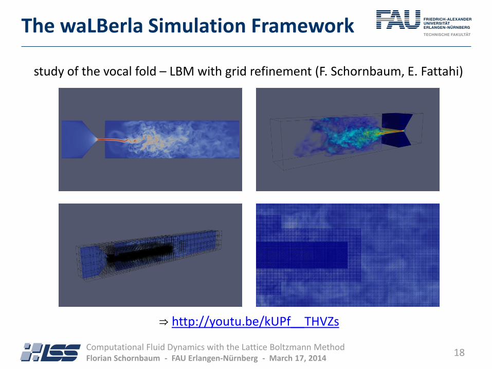
study of the vocal fold – LBM with grid refinement (F. Schornbaum, E. Fattahi)
Computational Fluid Dynamics with the Lattice Boltzmann Method Florian Schornbaum - FAU Erlangen-Nürnberg - March 17, 2014
study of the vocal fold – LBM with grid refinement (F. Schornbaum, E. Fattahi)
DNS (direct numerical simulation)
Reynolds number: 1000 / D3Q19 TRT
4300 processes @ SuperMUC
101,466,432 fluid cells
25,800 blocks with 16 x 16 x 16 cells
20
The waLBerla Simulation Framework
Computational Fluid Dynamics with the Lattice Boltzmann Method Florian Schornbaum - FAU Erlangen-Nürnberg - March 17, 2014
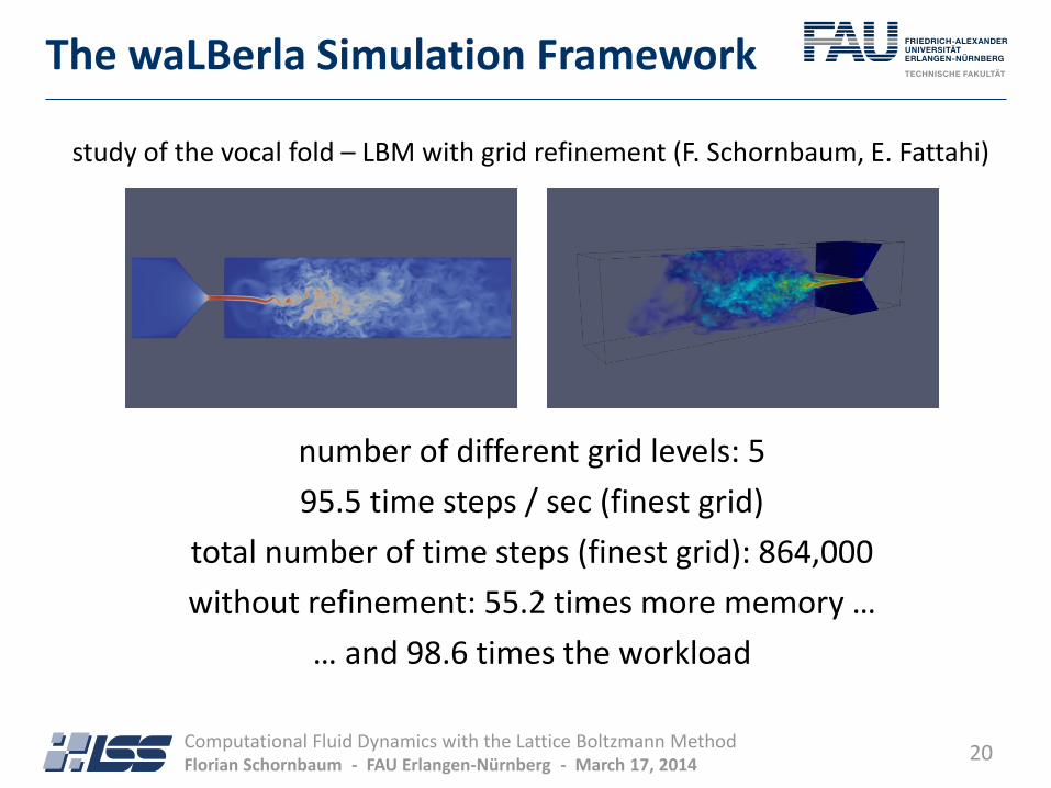
study of the vocal fold – LBM with grid refinement (F. Schornbaum, E. Fattahi)
number of different grid levels: 5
95.5 time steps / sec (finest grid)
total number of time steps (finest grid): 864,000
without refinement: 55.2 times more memory …
… and 98.6 times the workload
Course Schedule
22
Course Schedule
Computational Fluid Dynamics with the Lattice Boltzmann Method Florian Schornbaum - FAU Erlangen-Nürnberg - March 17, 2014
Monday Tuesday Wednesday Thursday Friday
Introduction [Lecture]
LB [Lecture]
LB [Lecture]
HPC (MPI) [Lecture]
Project Presentations
C++ [Lecture]
C++ [Lecture]
LB [Lecture]
Work on Projects
Project Presentations
Lunch Break
Lunch Break
Lunch Break
Lunch Break
Lunch Break
Getting to Know the
Environment [Hands-On]
waLBerla Tutorials
[Hands-On]
Introduction of Projects Work on
Projects
Work on Projects
Work on Projects
Morning time slots: 900 – 1030 and 1100 – 1230
Lunch Break: 1230 – 1400
Afternoon: 1400 – 1800 (Friday: 1600)
Introduction to the Lattice Boltzmann Method
24 Computational Fluid Dynamics with the Lattice Boltzmann Method Florian Schornbaum - FAU Erlangen-Nürnberg - March 17, 2014
Introduction to the LBM
regular grid with multiple particle distribution functions per cell
particle distribution function
scalar value
different models: D2Q9, D3Q19, D3Q27,
…
Macroscopic quantities (velocity, density, …)
can be calculated from the particle distribution
functions.
=
25 Computational Fluid Dynamics with the Lattice Boltzmann Method Florian Schornbaum - FAU Erlangen-Nürnberg - March 17, 2014
Introduction to the LBM
regular grid with multiple particle distribution functions per cell
particle distribution function
scalar value
different models: D2Q9, D3Q19, D3Q27,
…
Macroscopic quantities (velocity, density, …)
can be calculated from the particle distribution
functions.
=
26 Computational Fluid Dynamics with the Lattice Boltzmann Method Florian Schornbaum - FAU Erlangen-Nürnberg - March 17, 2014
Introduction to the LBM
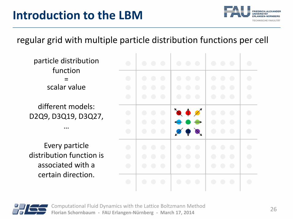
regular grid with multiple particle distribution functions per cell
particle distribution function
scalar value
different models: D2Q9, D3Q19, D3Q27,
…
Every particle distribution function is
associated with a certain direction.
=
27 Computational Fluid Dynamics with the Lattice Boltzmann Method Florian Schornbaum - FAU Erlangen-Nürnberg - March 17, 2014
Introduction to the LBM
explicit method → time stepping (separated into two steps)
two steps: stream & collide
streaming:
values are copied to neighboring cells
collision:
All values of each cell are updated using only the values of this cell. [cell-local operation!]
28 Computational Fluid Dynamics with the Lattice Boltzmann Method Florian Schornbaum - FAU Erlangen-Nürnberg - March 17, 2014
Introduction to the LBM
explicit method → time stepping (separated into two steps)
two steps: stream & collide
streaming:
values are copied to neighboring cells
collision:
All values of each cell are updated using only the values of this cell. [cell-local operation!]
29 Computational Fluid Dynamics with the Lattice Boltzmann Method Florian Schornbaum - FAU Erlangen-Nürnberg - March 17, 2014
Introduction to the LBM
explicit method → time stepping (separated into two steps)
two steps: stream & collide
streaming:
values are copied to neighboring cells
collision:
All values of each cell are updated using only the values of this cell. [cell-local operation!]
30 Computational Fluid Dynamics with the Lattice Boltzmann Method Florian Schornbaum - FAU Erlangen-Nürnberg - March 17, 2014
Introduction to the LBM
explicit method → time stepping (separated into two steps)
two steps: stream & collide
streaming:
values are copied to neighboring cells
collision:
All values of each cell are updated using only the values of this cell. [cell-local operation!]
For the collision, different operators exist: SRT, TRT, MRT
31 Computational Fluid Dynamics with the Lattice Boltzmann Method Florian Schornbaum - FAU Erlangen-Nürnberg - March 17, 2014
Introduction to the LBM
boundary treatment → pre-streaming step
Particle distribution functions are calcu-
lated for boundary cells which are neighboring
fluid cells.
These calculated values depend on the
underlying boundary condition type.
boundary
32 Computational Fluid Dynamics with the Lattice Boltzmann Method Florian Schornbaum - FAU Erlangen-Nürnberg - March 17, 2014
Introduction to the LBM
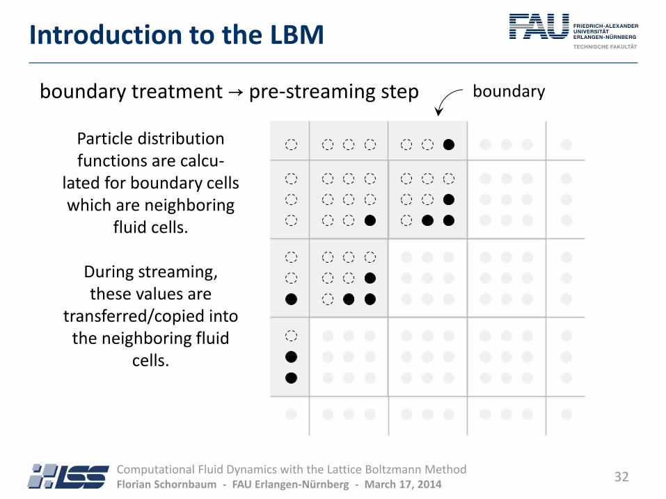
boundary treatment → pre-streaming step
Particle distribution functions are calcu-
lated for boundary cells which are neighboring
fluid cells.
During streaming, these values are
transferred/copied into the neighboring fluid
cells.
boundary
33 Computational Fluid Dynamics with the Lattice Boltzmann Method Florian Schornbaum - FAU Erlangen-Nürnberg - March 17, 2014
Introduction to the LBM
boundary treatment → pre-streaming step
Particle distribution functions are calcu-
lated for boundary cells which are neighboring
fluid cells.
During streaming, these values are
transferred/copied into the neighboring fluid
cells.
boundary
34 Computational Fluid Dynamics with the Lattice Boltzmann Method Florian Schornbaum - FAU Erlangen-Nürnberg - March 17, 2014
Introduction to the LBM
boundary treatment → pre-streaming step
Particle distribution functions are calcu-
lated for boundary cells which are neighboring
fluid cells.
During streaming, these values are
transferred/copied into the neighboring fluid
cells.
boundary
35 Computational Fluid Dynamics with the Lattice Boltzmann Method Florian Schornbaum - FAU Erlangen-Nürnberg - March 17, 2014
Introduction to the LBM
boundary treatment → pre-streaming step
The lattice Boltzmann method allows to
handle very complex geometries “easily”!
Cells are typically just
marked as being a boundary cell of a
certain type: no-slip, free slip, velocity
bounce-back, pressure, open boundary, …
[→ “flag field” = special grid that stores these markings]
boundary
36
• A typical time step of the LBM looks like as follows: 1. boundary treatment is performed (= values in the boundary cells
are prepared for streaming)
2. the streaming step is executed (requires nearest neighbor access)
3. the collision operator is evaluated (cell-local operation)
• A typical parallel time step includes communication: 1. all values of cells on the border of a process’s partition of the
domain are exchanged between neighboring processes (involves so-called ghost layer cells)
2. boundary treatment is performed (= values in the boundary cells
are prepared for streaming)
3. the streaming step is executed (requires nearest neighbor access)
4. the collision operator is evaluated (cell-local operation)
Introduction to the LBM
Computational Fluid Dynamics with the Lattice Boltzmann Method Florian Schornbaum - FAU Erlangen-Nürnberg - March 17, 2014
Introduction to waLBerla • Data Structures / Underlying Concepts
• Domain Decomposition & Parallelization
• A Prototypical Simulation
38
geometry given by surface mesh domain decomposition into blocks
empty blocks are discarded load balancing
Load balancing can be based on either space-filling curves (Z-order/Morton order, Hilbert curve) using the under-lying forest of octrees or graph partitioning (METIS, …).
Whatever fits best the needs of the simulation.
flow simulation only in here (example: complex geometry
of an artery)
Computational Fluid Dynamics with the Lattice Boltzmann Method Florian Schornbaum - FAU Erlangen-Nürnberg - March 17, 2014
Introduction to waLBerla
39
geometry given by surface mesh domain decomposition into blocks
empty blocks are discarded load balancing
Load balancing can be based on either space-filling curves (Z-order/Morton order, Hilbert curve) using the under-lying forest of octrees or graph partitioning (METIS, …).
Whatever fits best the needs of the simulation.
Computational Fluid Dynamics with the Lattice Boltzmann Method Florian Schornbaum - FAU Erlangen-Nürnberg - March 17, 2014
Introduction to waLBerla
40
geometry given by surface mesh domain decomposition into blocks
empty blocks are discarded load balancing
allocation of block data (→ grids)
The domain decomposition and load balancing can be performed during
the actual simulation … OR …
Computational Fluid Dynamics with the Lattice Boltzmann Method Florian Schornbaum - FAU Erlangen-Nürnberg - March 17, 2014
Introduction to waLBerla
41
geometry given by surface mesh domain decomposition into blocks
empty blocks are discarded load balancing
allocation of block data (→ grids)
DISK
separation of domain
partitioning from simulation
file size: kilobytes to few megabytes
DISK
Computational Fluid Dynamics with the Lattice Boltzmann Method Florian Schornbaum - FAU Erlangen-Nürnberg - March 17, 2014
Introduction to waLBerla
42
allocation of block data (→ grids)
DISK
separation of domain
partitioning from simulation
file size: kilobytes to few megabytes
DISK
empty blocks are discarded load balancing
geometry given by surface mesh domain decomposition into blocks
All of this (the entire pipeline) works just the same when grid
refinement is used.
Computational Fluid Dynamics with the Lattice Boltzmann Method Florian Schornbaum - FAU Erlangen-Nürnberg - March 17, 2014
• octree-like decomposition of the simulation space
special case of the much more general forest of
octrees data structure → non-uniform/refined grids
? ?
?
?
? ?
?
Introduction to waLBerla
Computational Fluid Dynamics with the Lattice Boltzmann Method Florian Schornbaum - FAU Erlangen-Nürnberg - March 17, 2014
forest of octrees: In general, each block contains
whatever data was registered by the application: can be any arbitrary
(sub)grid, scalar values, any object (in terms of C++), …
?
? ?
?
?
? ?
? ?
? ?
?
? ? ?
? ? ? ?
?
?
?
?
46
• Parallelization : • data exchange on borders between blocks via ghost layers
• typical parallelization of the underlying algorithm (e.g., LB): 1. perform communication: copy outermost layer of “inner” cells of
perform communication: sender to ghost layer of receiver
2. perform one time step of the computation algorithm only on all “inner” cells of each block → this computation algorithm is only allowed to access nearest neighbor cells during calculations!
Introduction to waLBerla
Computational Fluid Dynamics with the Lattice Boltzmann Method Florian Schornbaum - FAU Erlangen-Nürnberg - March 17, 2014
receiver process
sender process
(slightly more complicated for non-uniform domain decompositions, but the same general ideas still apply)
distribution of blocks to all available processes)
2. add data to blocks (LB: at least one grid that stores the particle
distribution functions and one grid that is used for marking cells as either being fluid or obstacle – additional grids/classes may be required/useful [e.g., an object that is responsible for the boundary treatment])
3. set-up geometry/boundaries (= mark cells as either being fluid or a
boundary of a certain type – information about the geometry/boundaries can be loaded from a mesh file, read in from a configuration file, set in the source code, etc.)
4. specify the algorithms/functions that are supposed to be executed in each time step (basic LB: communication, boundary
treatment, stream & collide, output[optional])
5. run the simulation = execute fixed number of time steps
Introduction to waLBerla
Computational Fluid Dynamics with the Lattice Boltzmann Method Florian Schornbaum - FAU Erlangen-Nürnberg - March 17, 2014