Computational Modelling 201 (Numerical Methods)jenlow/files/como201_lectures.pdf · Computational...

COMO 201: Numerical Methods and Structural Modelling, 2003 1

Computational Modelling 201

(Numerical Methods)

* DRAFT *Lecture Notes

Dr John EnlowLast modified July 22, 2003.

−2 −1.5 −1 −0.5 0 0.5 1 1.5 2

−2

−1.5

−1

−0.5

0

0.5

1

1.5

2

Contents

1 Preliminary Material 4

2 Introduction to Numerical Analysis 52.1 What is Numerical Analysis? . . . . . . . . . . . . . . . . . . . . . 5

2.1.1 Numerical Algorithms . . . . . . . . . . . . . . . . . . . . . 52.1.2 The Importance of Numerical Methods . . . . . . . . . . . . 7

2.2 Unavoidable Errors in Computing . . . . . . . . . . . . . . . . . . . 72.2.1 Floating Point Numbers . . . . . . . . . . . . . . . . . . . . 82.2.2 Roundoff (Machine) Error . . . . . . . . . . . . . . . . . . . 82.2.3 Truncation Error . . . . . . . . . . . . . . . . . . . . . . . . 92.2.4 Overflow and Underflow . . . . . . . . . . . . . . . . . . . . 92.2.5 Error Propagation . . . . . . . . . . . . . . . . . . . . . . . 9

3 Iteration and Root Finding 113.1 The Standard Iteration Method . . . . . . . . . . . . . . . . . . . . 113.2 Aitken’s Method for Acceleration (∆2 Method) . . . . . . . . . . . 13

3.2.1 The Mean Value Theorem (MVT) . . . . . . . . . . . . . . . 133.2.2 Aitken’s Approximate Solution . . . . . . . . . . . . . . . . 133.2.3 The ∆2 Notation . . . . . . . . . . . . . . . . . . . . . . . . 143.2.4 Aitken’s Algorithm . . . . . . . . . . . . . . . . . . . . . . . 15

3.3 Newton’s Method . . . . . . . . . . . . . . . . . . . . . . . . . . . . 153.3.1 Graphical Derivation of Newton’s Method . . . . . . . . . . 163.3.2 Pathological Failure of Newton’s Method . . . . . . . . . . . 173.3.3 Convergence Rate . . . . . . . . . . . . . . . . . . . . . . . . 18

3.4 Newton’s Method and Fractals . . . . . . . . . . . . . . . . . . . . . 183.5 Systems of Equations . . . . . . . . . . . . . . . . . . . . . . . . . . 20

3.5.1 Two Dimensions . . . . . . . . . . . . . . . . . . . . . . . . 203.5.2 Higher Dimensions . . . . . . . . . . . . . . . . . . . . . . . 223.5.3 Newton-Raphson Method for Nonlinear Systems of Equations 223.5.4 Example: Newton’s Method for Two Equations . . . . . . . 23

4 Interpolation and Extrapolation 254.1 Lagrange (Polynomial) Interpolation . . . . . . . . . . . . . . . . . 25

4.1.1 Examples of Lagrange Interpolation . . . . . . . . . . . . . . 274.2 Least Squares Interpolation . . . . . . . . . . . . . . . . . . . . . . 28

2


4.2.1 Fitting a Straight Line to Data (“Linear Regression”) . . . . 284.2.2 Least Squares from an Algebraic Perspective . . . . . . . . . 294.2.3 General Curve Fitting with Least Squares . . . . . . . . . . 31

5 Numerical Differentiation 325.1 Finite Differencing . . . . . . . . . . . . . . . . . . . . . . . . . . . 32

5.1.1 Second Derivative . . . . . . . . . . . . . . . . . . . . . . . . 335.2 Ordinary Differential Equations . . . . . . . . . . . . . . . . . . . . 33

5.2.1 High Order ODEs . . . . . . . . . . . . . . . . . . . . . . . . 335.2.2 Example: An Initial Value Problem (IVP) . . . . . . . . . . 33

6 Numerical Integration 356.1 The Trapezoid Rule . . . . . . . . . . . . . . . . . . . . . . . . . . . 356.2 Simpson’s Rule . . . . . . . . . . . . . . . . . . . . . . . . . . . . . 356.3 Gauss-Legendre Integration . . . . . . . . . . . . . . . . . . . . . . 36

6.3.1 Computational Determination of Weights and Nodes . . . . 37

7 Fundamentals of Statics and Equilibrium 407.1 Forces and Particles . . . . . . . . . . . . . . . . . . . . . . . . . . . 407.2 Newton’s Laws . . . . . . . . . . . . . . . . . . . . . . . . . . . . . 407.3 Static Equilibrium . . . . . . . . . . . . . . . . . . . . . . . . . . . 407.4 Solution of Mechanics Problems . . . . . . . . . . . . . . . . . . . . 41

7.4.1 SI Units in Mechanics . . . . . . . . . . . . . . . . . . . . . 417.5 More on Forces . . . . . . . . . . . . . . . . . . . . . . . . . . . . . 41

7.5.1 Coordinates . . . . . . . . . . . . . . . . . . . . . . . . . . . 427.5.2 Example I . . . . . . . . . . . . . . . . . . . . . . . . . . . . 437.5.3 Example II . . . . . . . . . . . . . . . . . . . . . . . . . . . 43

7.6 Equilibrium of a Particle . . . . . . . . . . . . . . . . . . . . . . . . 447.6.1 Example . . . . . . . . . . . . . . . . . . . . . . . . . . . . . 44

7.7 Free Body Diagrams . . . . . . . . . . . . . . . . . . . . . . . . . . 457.7.1 Example . . . . . . . . . . . . . . . . . . . . . . . . . . . . . 45

7.8 Rigid Bodies: Force Equivalents . . . . . . . . . . . . . . . . . . . . 467.8.1 Moment . . . . . . . . . . . . . . . . . . . . . . . . . . . . . 467.8.2 Varigon’s Theorem . . . . . . . . . . . . . . . . . . . . . . . 477.8.3 Equivalent Forces Theorem . . . . . . . . . . . . . . . . . . 487.8.4 Beam Corollary . . . . . . . . . . . . . . . . . . . . . . . . . 49

Chapter 1

Preliminary Material

Lecturer

First half: Dr John Enlow, Room 518, Science III ([email protected] ).Second half: Dr R.L. Enlow, Room 220, Science III.

Course structure:

• Two lectures (Tuesday and Thursday at 1pm, Seminar Room),

• One one-hour tutorial (not at the computers, Thursday 2pm, Seminar Room).

• One two-hour laboratory (using computers, Friday 10am-12pm, Lab A).

The tutorial exercise and the laboratory exercise are both due at 1pm on Friday.

Assessment:

The internal assessment is comprised of the mid-semester test (40%) and the weeklyexercises (60%). The final grade is either your final exam score or one third of yourinternal assessment plus two thirds of your final exam score, whichever is greater.

Computer Packages Used (First Half of Course)

All problems will be solved in, at your preference, MATLAB or C. It is assumedyou have good knowledge of one of these.

Books

There is no prescribed text for this half of the course. Useful references include:

• Numerical Recipes in C, Press, Teukolsky, Vetterling and Flannery.

• Numerical Methods with MATLAB, Recktenwald.

• Fundamentals of Computer Numerical Analysis, Freidman and Kandel.

4

Chapter 2

Introduction to NumericalAnalysis

2.1 What is Numerical Analysis?

Numerical analysis is a mathematical discipline. It is the study of numerical meth-

ods, which are mathematical techniques for generating approximate solutions toproblems (for example by using an iterative process or a series approximation).Numerical methods can be suitable for problems that are very difficult or impossi-ble to solve analytically.

2.1.1 Numerical Algorithms

Numerical methods are implemented via algorithms. An algorithm is a set of in-structions, each of which is composed of a sequence of logical operations. Theseinstructions use the techniques described by the numerical method to solve a prob-lem. A desired accuracy for the answer is generally specified, so that the algorithmterminates with an approximate solution after a finite number of steps.

An example of a numerical method is a scheme based on Newton’s methodto calculate

√a for any given a > 0. We assume that we are given an initial

estimation√

a ≈ x0. Each step of the algorithm consists of calculating xn+1,a (hopefully) better approximation to

√a, from the previous approximation

xn. This is done using the rule

xn+1 =1

2

(

xn +a

xn

)

, n ∈ N .

It can be shown that xn → √a as n → ∞. To enable an algorithm (which

implements the above method) to terminate after a finite number of steps,we might test xn after each step, stopping when

|xn − xn−1| < 10−6.

5


There is more to numerical analysis than just development of methods andalgorithms. We also need to know how to predict the behaviour of both the methodand its associated algorithms. Common questions include:

• Under what conditions will the method/algorithm produce a correct approx-imate solution to the problem? (e.g. convergence issues, stability).

• What can we say about the errors in the approximate solutions? (error anal-ysis).

• How long does it take to find a solution to a given accuracy? (O(n log(n))etc...).

Answering these questions may well be more difficult than developing either themethod or algorithm, and the answers are often non-trivial.

For example, consider the standard iterative method for solving x = f(x)on a ≤ x ≤ b (where at each step we calculate xn+1 = f(xn)). Sufficientconditions for both a unique solution to exist and for the method to beguaranteed to converge to this unique solution are:

1. f(x) continuous on [a, b],

2. x ∈ [a, b] ⇒ f(x) ∈ [a, b],

3. ∃L ∈ R, ∀x ∈ [a, b], |f ′(x)| ≤ L < 1.

g(x) ≡ x

f(x)

x

y

This course will focus on numerical methods and algorithms rather than on nu-merical analysis. MATH 361, which some of you will take in first semester 2003,focuses on numerical analysis. It provides a greater depth of understanding of thederivation of the methods and of their associated errors and limitations. Numericalanalysis does not require the use of a computer because it focuses on theoretical


ideas. In contrast we will make regular use of computers in this course, spendingroughly 2

3of the exercise time in Lab A.

2.1.2 The Importance of Numerical Methods

Computers are used for a staggering variety of tasks, such as:

• accounting and inventory control,

• airline navigation and tracking systems,

• translation of natural languages,

• monitoring of process control and

• modelling of everything from stresses in bridge structures during earthquakesto possum breeding habits.

One of the earliest and largest uses of computers is to solve problems in scienceand engineering. The techniques used to obtain such solutions are part of thegeneral area called scientific computing, which in turn is a subset of computational

modelling, where a problem is modelled mathematically then solved on computer(the solution process being scientific computing).

Nearly every area of modern industry, science and engineering relies heavily oncomputers. In almost all applications of computers, the underlying software relieson mathematically based numerical methods and algorithms. While examples donein this course focus on solving seemingly simple mathematical problems with nu-merical methods, the importance of these same methods to aspects of an enormousrange of real world problems can not be overstated. An understanding of thesefundamental ideas will greatly assist you in using complex and powerful computerpackages designed to solve real problems. They are also a crucial component ofyour ability, as computational modelers, to solve modelled systems.

2.2 Unavoidable Errors in Computing

Representation of modelled systems in a computer introduces several sources oferror, primarily due to the way numbers are stored in a computer. These sourcesof error include:

• Roundoff or Machine error.

• Truncation error.

• Propagated errors.


2.2.1 Floating Point Numbers

DefinitionThe representation of a number f as

f = s · m · Mx

where

• the sign, s, is either +1 or −1,

• the mantissa, m, satisfies 1/M ≤ m ≤ 1,

• the exponent, x, is an integer,

is called the floating point representation of f in base M .

The decimal number f = 8.75, written in its floating point representationin base 10 is 0.875 · 101, and has s = 1, m = 0.875 and x = 1. Its binaryequivalent is

f = (1000.11)2 = +(0.100011)2 · (2)(100)2

where s = 1, m = (0.100011)2 and x = (100)2.

2.2.2 Roundoff (Machine) Error

In a computer the mantissa m of a number x is represented using a fixed number ofdigits. This means that there is a limit to the precision of numbers represented in acomputer. The computer either truncates or rounds the mantissa after operationsthat produce extra mantissa digits.

The absolute error in storing a number on computer in base 10 using d digitscan be calculated as follows. Let m be the truncated mantissa, then the magnitudeof the absolute error is

ε = |s · m · 10x − s · m · 10x| = |m − m| · 10x < 10−d10x

Roundoff error can be particularly problematic when a number is subtracted froman almost equal number (subtractive cancellation). Careful algebraic rearrangementof the expressions being evaluated may help in some cases.

The expression

1015 ∗ (pi − 3.14159265359) = −206.7615373566167...

However when evaluated on my calculator the answer given is 590, 000!!Clearly the calculator’s answer is catastrophically incorrect.


2.2.3 Truncation Error

This type of error occurs when a computer is unable to evaluate explicitly a givenquantity and instead uses an approximation.

For example, an approximation to sin(x) might be calculated using thefirst three terms of the Taylor series expansion,

sin(x) = x − x3

3!+

x5

5!+ E(x)

where

|E(x)| ≤ x7

7!.

If x is in the interval [−0.2, 0.2] then the truncation error for this operationis at most

0.27

7!< 3 · 10−9

2.2.4 Overflow and Underflow

Underflow and overflow errors are due to a limited number of digits being assignedto the exponent, so that there is a largest and smallest magnitude number that canbe stored (N and M say). Attempts to store a number smaller than M will resultin underflow, generally causing the stored number to be set to zero. Overflow errorsare more serious, occurring when a calculated or stored number is larger than N .These generally cause abnormal termination of the code.

Consider the modulus of a complex number a + ib. The obvious way tocalculate this is using

|a + ib| =√

a2 + b2,

however this method is clearly prone to overflow errors for large a or b. Amuch safer approach is with the relation

|a + ib| =

|a|√

1 + (b/a)2, |a| ≥ |b|

|b|√

1 + (a/b)2, |a| < |b|

2.2.5 Error Propagation

Errors in calculation and storage of intermediate results propagate as the calcula-tions continue. It is relatively simple to derive bounds on the propagated errorsafter a single operation, but combining many operations can be problematic andmay lead to complicated expressions.


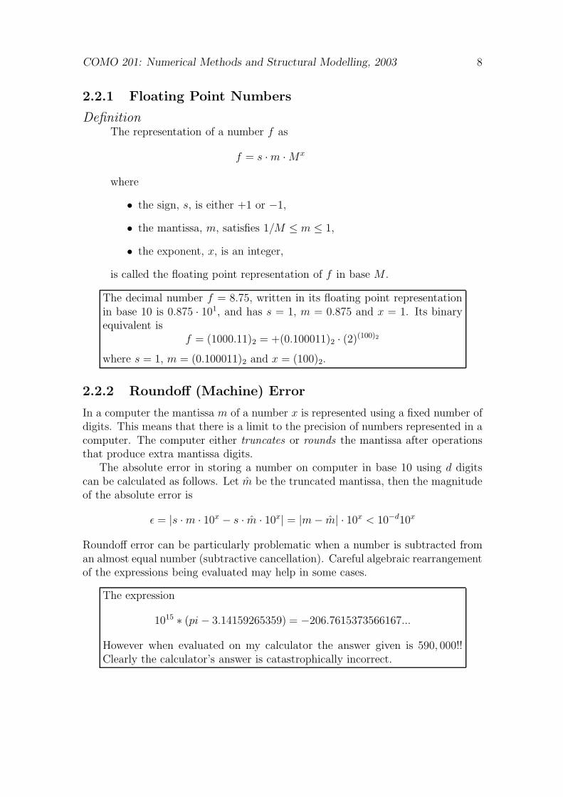
Consider quantities x and y approximating ideal values x and y. Let εx andεy be bounds on the magnitudes of the absolute errors in these approxima-tions, so that

|x − x| ≤ εx, |y − y| ≤ εy.

Then, using the triangle inequality, the propagated error under the additionoperation is

|(x + y) − (x + y)| ≤ |x − x| + |y − y| ≤ εx + εy.

Chapter 3

Iteration and Root Finding

Solving nonlinear equations is a major task of numerical analysis and the iterationmethod is a prototype for many methods dealing with these equations.

3.1 The Standard Iteration Method

The standard iteration method is designed to solve equations of the form

x = f(x)

where f(x) is a real valued function defined over some interval [a, b].

An algorithm for the standard iteration method.

1. Choose an initial approximate solution x0, a tolerance ε and a maxi-mal number of iterations N . Set n = 1.

2. Create the next iteration using the relation

xn = f(xn−1).

3. If |xn − xn−1| > ε and n < N then increment n and go to step 2.

4. If |xn − xn−1| > ε then the maximal number of iterations has beenreached without the desired convergence. Raise a warning that thisis the case.

5. Output xn, the approximate solution to x = f(x).

Clearly the algorithm finishes when successive approximations are less than ε apart.Ideally we have

limn→∞

xn = s, where s = f(s)

11


and |xn−s| monotonically decreasing as n increases. In fact we have already stateda theorem that gives us sufficient conditions for behaviour similar to this - see theexample in section 2.1.1.

Example where |f ′(x)| < 1 on the interval. Good convergence.

f(x) = E−x +1

10sin(10x), x0 =

1

5

0.2 0.4 0.6 0.8 1

0.2

0.4

0.6

0.8

1

Example where ∃x ∈ [0, 1] s.t. |f ′(x)| > 1. Poor convergence!

f(x) = E−x +1

5sin(20x), x0 =

1

5

0.2 0.4 0.6 0.8 1

0.2

0.4

0.6

0.8

1


3.2 Aitken’s Method for Acceleration (∆2 Method)

Aitken’s ∆2 method improves on the convergence rate of the S.I.M. in cases wherethe S.I.M. converges to a unique solution. It does this by generating an approximateexpression for f ′(s), then using this information to predict what the S.I.M. is goingto converge to. In deriving Aitken’s method we’ll need to use the mean valuetheorem.

3.2.1 The Mean Value Theorem (MVT)

Recall the Mean Value Theorem (M.V.T):Let f(x) be differentiable on the open interval (a, b) and continuous on the closed

interval [a, b]. Then there is at least one point c in (a, b) such that

f ′(c) =f(b) − f(a)

b − a

a bc1 c2

f(x)

x

y

f(a)

f(b)

3.2.2 Aitken’s Approximate Solution

Let f be a ‘nice’ function, with both f(x) and f ′(x) continuous and differentiable inthe domain of interest. Suppose that we have an approximation xa to the solutions (where f(s) = s). Assume that the S.I.M., starting at xa will converge to s. Letxb and xc represent two iterations of the S.I.M., so that xb = f(xa) and xc = f(xb).Then for some ca between xa and s,

xb − s = f(xa) − f(s) = (xa − s) f ′(ca) by the M.V.T. (3.1)


and similarly, for some cb between xb and s,

xc − s = (xb − s) f ′(cb) (3.2)

Both xa and xb are close to s, since xa is an approximate solution, so that ca and cb

are also close to s (because |ca − s| < |xa − s| and |cb − s| < |xb − s|). With this inmind, we approximate f ′(ca) and f ′(cb) by f ′(s) in equations 3.1 and 3.2, giving:

xb − s ≈ (xa − s) f ′(s) (3.3)

xc − s ≈ (xb − s) f ′(s) (3.4)

Subtracting Eq. 3.3 from Eq. 3.4 yields:

f ′(s) ≈ xc − xb

xb − xa

Substituting this expression back into Eq. 3.3 and rearranging yields the followingapproximate solution to f(x) = x.

s ≈ x∗ ≡ xa −(xb − xa)

2

xc − 2xb + xa

In general x∗ will be much closer to s than xa, xb and xc. We use this expressionroughly as follows:

• Start at an estimated solution xa.

• At each iteration calculate xb = f(xa), xc = f(xb) and x∗ (using the boxedequation above).

• Set xa for the next iteration to be the current value of x∗.

Before developing a full algorithm we’ll explain why this method is called Aitken’s∆2 method.

3.2.3 The ∆2 Notation

This expression can be written more compactly using the forward difference operator

∆, which is defined by the three relations:

∆xn ≡ xn+1 − xn, n ≥ 0

∆

m∑

j=1

αjxnj

≡m

∑

j=1

αj∆xnj, m ≥ 1, αj ∈ R, (∀j) nj ≥ 0

∆nE ≡ ∆(

∆n−1E)

, n ≥ 2

The more compact form of the boxed equation, which gives the method its name,is given by

x∗ = xa −(∆xa)

2

∆2xa.


3.2.4 Aitken’s Algorithm

Aitken’s algorithm is as follows. x∗a represents Aitken’s accelerated approximate

solution, xb and xc are two iterations of the S.I.M. starting at x∗a.

1. Choose an initial approximate solution x∗a, a tolerance ε and a maximal num-

ber of iterations N . Set n = 0.

2. Compute xb = f(x∗a) and xc = f(xb).

3. Update x∗a with x∗

a = x∗a −

(xb − x∗a)

2

xc − 2xb + x∗a

4. Increment n.

5. If |f(x∗a) − x∗

a| > ε and n < N then go to step 2.

6. If |f(x∗a)−x∗

a| > ε then raise a warning that the maximal number of iterationshas been reached without the desired convergence.

7. Output the approximate solution x∗a.

3.3 Newton’s Method

Newton’s method, sometimes called the Newton-Raphson method, is designed tofind solutions of the equation

f(x) = 0,

where f(x) is some function whose roots are non-trivial to find analytically. Supposethat we have already iterated a number of times, arriving at our approximation xk

to the true solution. Ideally the next iteration of the method will choose xk+1 sothat f(xk+1) = 0. If we approximate f(xk+1) using known quantities, then set thisapproximation to zero, we can solve for a good value of xk+1 (so that f(xk+1) ≈ 0).But what approximation should we use?

Newton’s method arises from approximating f(xk+1) using a Taylor series off(x) expanded about xk. Using the standard forward difference operator ∆, sothat ∆xk ≡ xk+1 − xk, this Taylor series is

f(xk+1) = f(xk + ∆xk) = f(xk) + ∆xkdf

dx

∣

∣

∣

∣

∣

xk

+(∆xk)

2

2

d2f

dx2

∣

∣

∣

∣

∣

xk

+ . . .

Assuming that ∆xk is small, i.e. that we are close to the solution, f(xk+1) can beapproximated using the first two terms:

f(xk+1) ≈ f(xk) + ∆xkdf

dx

∣

∣

∣

∣

∣

xk


Setting this approximation of f(xk+1) to zero gives

f(xk) + (xk+1 − xk)df

dx

∣

∣

∣

∣

∣

xk

= 0

and solving for xk+1 yields

xk+1 = xk −f(xk)

f ′(xk).

This iteration is the basis of Newton’s method.

3.3.1 Graphical Derivation of Newton’s Method

Consider a root-finding method which sets xk+1 to be the intercept of the tangentline to f(x) at xk with the x-axis.

y

xxk+1xk

f(xk)

f(x)

slope =∆y

∆x

⇒ f ′(xk) =0 − f(xk)

xk+1 − xk

⇒ f ′(xk)(xk+1 − xk) = −f(xk)

⇒ xk+1 − xk = − f(xk)

f ′(xk)

and so

xk+1 = xk −f(xk)

f ′(xk).


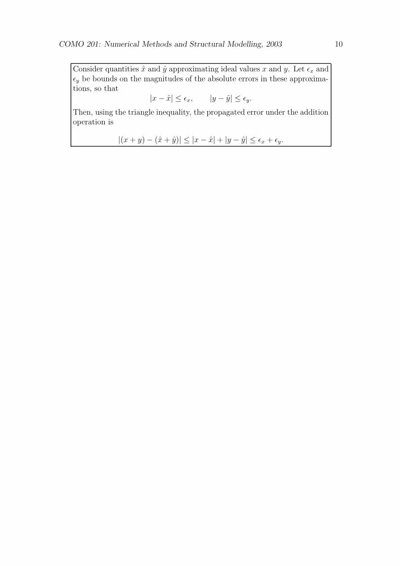
3.3.2 Pathological Failure of Newton’s Method

How else could Newton’s method fail?

• Divergence:y

x

f(x0)

x1x0

f(x1)

f(x)

• Cycles / oscillation:y

f(x1)

f(x0)

x

f(x)

x0, x2, x4, . . . x1, x3, x5, . . .

• Poor convergence (near zero slope).

The issues are often located near turning points.


3.3.3 Convergence Rate

Newton’s method has quadratic convergence1 when close to the root2 - the error atstep k + 1 is of the order of the square of the error at step k. This is much betterthan the other methods described (including Aitken’s ∆2 method) which only havelinear convergence.

3.4 Newton’s Method and Fractals

−2 −1.5 −1 −0.5 0 0.5 1 1.5 2

−2

−1.5

−1

−0.5

0

0.5

1

1.5

2

The fractal shown is obtained by considering Newton’s method when used onthe complex -valued equation

z3 − 1 = 0.

1In the case of repeated roots we have f ′(x) = 0 at the roots, meaning that Newton’s methodonly manages linear convergence.

2Choosing a starting value close to the root is very important. Newton’s method depends ona good starting value for convergence.


Newton’s method gives the iteration

zj+1 = zj −z3

j − 1

3z2j

.

Looking at the region |z| < 2, we colour a pixel white if Newton’s method convergesto z = 1 and black if it converges to one of the two complex roots. All pointsconverge, with the exception of the origin and three points along the negative realaxis. Although we may have expected the three regions (one for each root) to beidentically shaped due to symmetry, the fractal behaviour is quite surprising! Pointsnear local extrema cause Newton’s method to shoot off towards other remote values.

Source File: nfrac.mfunction.nfrac

%.Generates.a.fractal.based.on.which.root.Newton’s.

%.method.converges.to.when.considering.

%..........f(z).=.z^3.-.1.

%.We.colour.anything.converging.to.z=1.(the.real.root).black.

n=500;.m=zeros(n,n);

for.(it1=1:n)

.....for.(it2=1:n)

..........x.=.((it1-1)/(n-1).-0.5)*4;.

..........y.=.((it2-1)/(n-1).-0.5)*4;

..........if.(x*x+y*y<4)

..................m(it2,it1)=getcolour(.x.+.i.*.y.);

..........else

...............m(it2,it1)=0.5;

..........end

.....end

end

imagesc([-2.2],.[-2.2],m);

colormap(gray);

axis.square;

%------------------------------------------------------------

function.[.thecolour.].=.getcolour(.zz.)

%.This.calculates.20.iterations.of.Newton’s.method.

iterations=20;

thecolour=0;..%.Black.by.default.

for.u=1:iterations

....zz.=.zz.-.(zz^3.-.1)/(3.*.zz^2);

end

if.(abs(zz-1)<0.1).thecolour.=.1;.end.%.White.if.zz.~=.1.


3.5 Systems of Equations

Newton’s method can easily be applied to systems of nonlinear equations.

3.5.1 Two Dimensions

Consider the simultaneous equations

f(x, y) = 0, and g(x, y) = 0.

We can think of the equation f(x, y) = 0 as representing a “level curve” at z = 0of the function z = f(x, y). This level curve is the intersection of the functionz = f(x, y) with the z = 0 plane. Consider for example f(x, y) = x2 + y2− 3. Then

f(x, y) = 0 ⇒ x2 + y2 − 3 = 0 ⇒ x2 + y2 = 3,

and so the level curve is a circular region in the x, y-plane.

In[12]:= Plot3D@x^2 + y^2 - 3, 8x, -Pi, Pi<, 8y, -Pi, Pi<D;

-2

0

2-2

0

205

1015

-2

0

2

In[13]:= ContourPlot@x^2 + y^2 - 3, 8x, -Pi, Pi<, 8y, -Pi, Pi<,Contours ® 80<, ContourShading ® False, PlotPoints ® 50D;

-3 -2 -1 0 1 2 3

-3

-2

-1

0

1

2

3


Similarly the equation g(x, y) = 0 represents a level curve of z = g(x, y). Thesimultaneous solution of f(x, y) = 0 and g(x, y) = 0 then represents the intersectionpoints of the two corresponding level curves.

For example, with f(x, y) = x2 + y2 − 3 and g(x, y) = 2x2 + 14y2 − 3, we have:

-3 -2 -1 0 1 2 3

-3

-2

-1

0

1

2

3

Level Curve at z=0 for z=2x^2+Hy�2L^2-3

-2 -1 0 1 2 3

-2

-1

0

1

2

3

Generally speaking the two curves representing f = 0 and g = 0 have no relationto each other at all! Graphically, Newton’s method in two dimensions works by:

1. Starting with an approximate solution (xk, yk).

2. Calculating the tangent planes to the surfaces z = f(x, y) and z = g(x, y).

3. Calculating the lines of intersection of the planes with the x, y-plane.

4. Calculating the intersection of the two lines. This intersection point is thenew approximate solution (xk+1, yk+1).


3.5.2 Higher Dimensions

In higher dimensions the situation quickly gets more complicated. In three dimen-sions we’re looking at intersections of three level surfaces. Graphical interpretationof the method becomes extremely difficult. However, computationally, Newton’smethod in any dimension can calculated with one algorithm!

3.5.3 Newton-Raphson Method for Nonlinear Systems ofEquations

A typical problem gives N equations to be solved in variables x1, x2, . . . , xN :

F1(x1, x2, . . . , xN) = 0

F2(x1, x2, . . . , xN) = 0...

......

FN (x1, x2, . . . , xN) = 0

Or, written more compactly,

Fi(x1, x2, . . . , xN) = 0, i = 1, 2, . . . , N.

The Taylor series for each component of ~F = (F1, F2, . . . , FN) expanded about~x = (x1, x2, . . . , xN ) is given in terms of the column vector δ~x by

Fi(~x + δ~x) = Fi(~x) + ~Ji · δ~x + O(|δ~x|2)where the row vector ~Ji is given by ~Ji =

[

∂Fi

∂x1

, ∂Fi

∂x2

, . . . , ∂Fi

∂xN

]

and O(|δ~x|2) means

terms with total magnitude of the order of |δ~x|2 .We then have the approximation

Fi(~x + δ~x) ≈ Fi(~x) + ~Ji · δ~x.

Let J be the matrix with rows ~J1, . . . , ~JN , i.e. with elements

Ji,j ≡∂Fi

∂xj

,

then setting Fi(~x + δ~x) to zero gives

J δ~x = −~F .

This is the basis of the multidimensional form of Newton’s method. Suppose, start-ing from ~x0, that we have reached iteration k giving approximate solution ~xk. Thenthe next step is calculated as follows.

1. Calculate ~F (~xk).

2. Calculate the Jacobian matrix J at ~x = ~xk.

3. Solve J δ~xk= −~F (~xk) for δ~xk

(e.g. with an LU decomposition).

4. Set ~xk+1 = ~xk + δ~xk.

We stop iterating when ||~xk+1 − ~xk|| is smaller than a specified tolerance.


3.5.4 Example: Newton’s Method for Two Equations

Consider the example described previously:

F1(x, y) = x2 + y2 − 3, F2(x, y) = 2x2 +1

4y2 − 3,

where we wish to find x and y such that F1(x, y) = 0 and F2(x, y) = 0. Thus

~F ≡[

F1

F2

]

=

[

x2 + y2 − 32x2 + 1

4y2 − 3

]

The Jacobian matrix is then

J ≡

∂F1

∂x∂F1

∂y

∂F2

∂x∂F2

∂y

=

2x 2y

4x 12y

The main step of the algorithm , J · δ~xk= −~F (~xk) can be solved using the inverse

of the matrix J when it exists:

δ~xk= −J−1 · ~F (~xk)

⇒[

δx

δy

]

= −

2x 2y

4x 12y

−1

x2 + y2 − 3

2x2 + 14y2 − 3

⇒[

δx

δy

]

=

114x

− 27x

− 47y

27y

x2 + y2 − 3

2x2 + 14y2 − 3

⇒[

δx

δy

]

=

914x

− x2

67y

− y2

and so

xk+1

yk+1

=

xk

yk

+

914xk

− xk

2

67yk

− yk

2

Iterating in Mathematica, starting at (x0, y0) = (−1, 2):

In[19]:= newtstep@8xk_, yk_<D := 8xk + 9� H14 xkL - xk�2, yk + 6� H7 ykL - yk�2<;In[23]:= NestList@newtstep, 8-1.0, 2.0<, 4D �� MatrixForm

Out[23]//MatrixForm=ikjjjjjjjjjjjjjjjj

-1. 2.-1.14286 1.42857-1.13393 1.31429-1.13389 1.30932-1.13389 1.30931

y{zzzzzzzzzzzzzzzz


Newton’s Method in Mathematica

Mathematica’s FindRoot command uses Newton’s method.

In[1]:=

FindRoot[{2 x^2 + (y/2)^2 - 3 == 0, x^2 + y^2 - 3 == 0},{x, -1}, {y, 2}]

Out[1]= {x -> -1.13389, y -> 1.30931}

-2 -1 0 1 2 3

-2

-1

0

1

2

3

Newton’s Method in MATLAB

MATLAB’s fzero command uses a competing scheme restricted to one dimension.Multidimensional methods require the Optimization toolbox or custom routines.

Source File: newtdemo.mfunction.newtdemo

%.solving.f(x,y).=.x^2.+.y^ 2.-.3..=.0,.

%.........g(x,y).=.2.x^2.+.(y/2)^2..-.3..=.0

%.starting.at.x=-1,.y=2.

vals.=.[-1.;.2];

for.(loopy=1:10)

.....vals.=.newtstep(vals);

end

vals.....%.display.the.final.approximation.

%.ONE.ITERATION.OF.NEWTON’S.METHOD.

function.newvals.=.newtstep(oldvals)

x.=.oldvals(1);.y.=.oldvals(2);

F.=.[.x^2.+.y^2.-.3.;.2*x^2.+.(y/2)^2..-.3.];

J.=.[.2*x.,.2*y.;..4*x..,.y/2...];

deltax.=.-J.\.F;...%.MATLAB’s.left.matrix.divide.

newvals.=.oldvals.+.deltax;

>> format long

>> newtdemo

vals =

-1.13389341902768

1.30930734141595

Chapter 4

Interpolation and Extrapolation

• Used when we know values of a function f(x) at a set of discrete pointsx1, x2, . . . , xN but we don’t have an analytic expression for f(x) that lets uscalculate its value at an arbitrary point.

• If we want to find f(x) at one or more values of x outside the interval [x1, xN ]then the problem is called extrapolation. If x ∈ [x1, xN ] it’s interpolation.

• The general idea is to fit some smooth function to the data points. Typicalfunctions used include:

1. Polynomials (by far the most common method).

2. Rational Functions (quotients of polynomials).

3. Trigonometric functions (sines and cosines, giving rise to trigonometric

interpolation and related Fourier methods).

4.1 Lagrange (Polynomial) Interpolation

Suppose that we have N points, (x1, y1), (x2, y2), . . . (xN , yN) and wish to find theunique polynomial of degree N − 1 that passes through them. We write this poly-nomial in terms of the y1, . . . , yN values as:

P (x) =N

∑

k=1

gk(x) yk.

Since we want p(x) to pass through our N points, we need

P (xi) = yi =N

∑

k=1

gk(xi) yk.

This clearly holds if we choose our gk functions so that

gk(xi) =

{

1 if i = k0 if i 6= k

25


because

P (xi) =N

∑

k=1

gk(xi) yk = g1(xi)y1 + g2(xi)y2 + . . . + gi(xi)yi + . . . + gN(xi)yN

= 0y1 + 0y2 + . . . + 1yi + . . . + 0yN

= yi

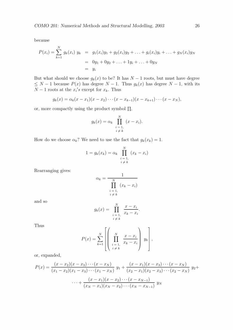
But what should we choose gk(x) to be? It has N − 1 roots, but must have degree≤ N − 1 because P (x) has degree N − 1. Thus gk(x) has degree N − 1, with itsN − 1 roots at the xi

′s except for xk. Thus

gk(x) = αk(x − x1)(x − x2) · · · (x − xk−1)(x − xk+1) · · · (x − xN ),

or, more compactly using the product symbol∏

,

gk(x) = αk

N∏

i = 1,i 6= k

(x − xi).

How do we choose αk? We need to use the fact that gk(xk) = 1.

1 = gk(xk) = αk

N∏

i = 1,i 6= k

(xk − xi)

Rearranging gives:

αk =1

N∏

i = 1,i 6= k

(xk − xi)

and so

gk(x) =N∏

i = 1,i 6= k

x − xi

xk − xi

.

Thus

P (x) =N

∑

k=1

N∏

i = 1,i 6= k

x − xi

xk − xi

yk

,

or, expanded,

P (x) =(x − x2)(x − x3) · · · (x − xN )

(x1 − x2)(x1 − x3) · · · (x1 − xN )y1 +

(x − x1)(x − x3) · · · (x − xN )

(x2 − x1)(x2 − x3) · · · (x2 − xN )y2+

· · ·+ (x − x1)(x − x2) · · · (x − xN−1)

(xN − x1)(xN − x2) · · · (xN − xN−1)yN


4.1.1 Examples of Lagrange Interpolation

1. Clearly y = x2 goes through the points (−1, 1), (0, 0), and (1, 1). Checkingthat Lagrangian interpolation gives x2:

g1(x) =n

∏

i=2

x − xi

x1 − xi

=(x − 0)(x − 1)

(−1 − 0)(−1 − 1)=

1

2x2 − 1

2x

g2(x) =(x − (−1))(x − 1)

(0 − (−1))(0 − 1)= 1 − x2

g3(x) =(x − (−1))(x − 0)

(1 − (−1))(1 − 0)=

1

2x2 +

1

2x

⇒ p(x) = g1(x) · 1 + g2(x) · 0 + g3(x) · 1 =1

2

(

x2 − x + x2 + x)

= x2

• In Mathematica with a custom Lagrangian interpolation function:

In[113]:= Clear@pD;p@xl_, yl_D := ModuleA8n = Length@xlD<, ExpandA

ãk=1

n ikjjjjjjylPkT äi=1

n-1 x - Drop@xl, 8k<DPiT��xlPkT - Drop@xl, 8k<DPiT y{zzzzzzEE;

In[115]:= p@8-1, 0, 1<, 81, 0, 1<DOut[115]= x2

• In MATLAB with polyfit:

>> x=[-1 0 1]; y=[1 0 1]; polyfit(x,y,2)

ans =

1.0000 0.0000 0

2. Find the cubic through the points (1, 20), (2, 40), (4, 140), and (6, 200).

• In Mathematica with the above function:

In[94]:= p@8 8 1, 20<, 82, 40<, 84, 140<, 86, 200<<DOut[94]= 44 - 52 x + 31 x2 - 3 x3

• In Mathematica least squares curve fitting:

Fit@881, 20<, 82, 40<, 84, 140<, 86, 200<<,81, x, x2, x3<, xDOut[97]= 44. - 52. x + 31. x2 - 3. x3

• In MATLAB with polyfit:

>> x=[1 2 4 6]; y=[20 40 140 200]; polyfit(x,y,3)

ans =

-3.0000 31.0000 -52.0000 44.0000


4.2 Least Squares Interpolation

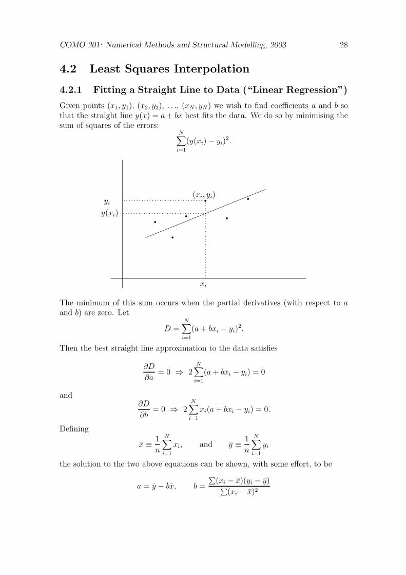
4.2.1 Fitting a Straight Line to Data (“Linear Regression”)

Given points (x1, y1), (x2, y2), . . ., (xN , yN) we wish to find coefficients a and b sothat the straight line y(x) = a + bx best fits the data. We do so by minimising thesum of squares of the errors:

N∑

i=1

(y(xi) − yi)2.

xi

yi

y(xi)

(xi, yi)

The minimum of this sum occurs when the partial derivatives (with respect to aand b) are zero. Let

D =N

∑

i=1

(a + bxi − yi)2.

Then the best straight line approximation to the data satisfies

∂D

∂a= 0 ⇒ 2

N∑

i=1

(a + bxi − yi) = 0

and∂D

∂b= 0 ⇒ 2

N∑

i=1

xi(a + bxi − yi) = 0.

Defining

x ≡ 1

n

N∑

i=1

xi, and y ≡ 1

n

N∑

i=1

yi

the solution to the two above equations can be shown, with some effort, to be

a = y − bx, b =

∑

(xi − x)(yi − y)∑

(xi − x)2


4.2.2 Least Squares from an Algebraic Perspective

Suppose we have a set of overly constrained (inconsistent) equations written as amatrix equation:

A~v = ~b

where ~v and ~b are column vectors. The optimal solution, in the least squares sense,will minimise the sum of the squares of the errors, i.e. minimise

∑

i

ε2i = |~ε |2, where ~ε = A~v −~b.

This is equivalent to finding the minimum of

|~ε | = |A~v −~b|.

This minimising value of ~v, ~v∗ say, occurs when the corresponding ~ε∗ is perpendicularto the column space1 of A, as can be seen geometrically:

Column space of A

~bA~x∗

~ε∗ = A~x∗ −~b

Thus ~ε∗ is orthogonal to every column A(:, j) =

A1,j

A2,j...

Am,j

i.e.,

∀j ∈ {1, 2, . . . , n} , [A1,j A2,j . . . Am,j]

ε∗1ε∗2...

ε∗m

= 0,

and soAT~ε∗ = ~0.

1The column space of A is the set of all vectors which can be formed by linear combinationsof the columns of A.


Thus the optimal value ~v = ~v∗ satisfies

AT (A~v∗ − b) = 0

⇒ AT A~v∗ = AT~b

⇒ ~v∗ = (AT A)−1AT~b

It can be shown that the inverse (AT A)−1 exists if all columns of A are independent.

Application

Suppose that a linear relation is anticipated between two variables x and y ofwhich we have a number of measurements (x1, y1) through to (xN , yN). Let therelationship be expressed in the form y = a + bx. The “unsolvable” system that wewant a closest solution to is:

1 x1

1 x2...

...1 xN

[

ab

]

=

y1

y2...

yN

Then the optimal solution [a∗ b∗]T is given by:

[

1 1 . . . 1x1 x2 . . . xN

]

1 x1

1 x2...

...1 xN

[

a∗

b∗

]

=

[

1 1 . . . 1x1 x2 . . . xN

]

y1

y2...

yN

Or, more compactly,

N∑

xi

∑

xi∑

x2i

a∗

b∗

=

∑

yi

∑

xi yi

We could invert to find the general solution, or alternatively solve the two simulta-neous equations for a∗ and b∗. The latter gives:

Na∗ + Nxb∗ = Ny and Nxa∗ +∑

x2i b

∗ =∑

xiyi.

The first equation readily yields a∗ = y − b∗x, as we had before. The second thengives

Nx(y − b∗x) +∑

x2i b

∗ =∑

xiyi

⇒ (∑

x2i − Nx2)b∗ =

∑

xiyi − Nxy

and so

b∗ =

∑

xiyi − Nxy∑

x2i − Nx2


The numerator can be re-expressed as∑

xiyi − Nxy =∑

xiyi + Nxy − Nxy − Nxy

=∑

xiyi +∑

xy −∑

xyi −∑

yxi

=∑

(xiyi + xy − xyi − yxi)

=∑

(xi − x) (yi − y)

Similarly the denominator satisfies∑

x2i − Nx2 =

∑

(xi − x)2 which gives us thefamiliar expression for b∗,

b∗ =

∑

(xi − x)(yi − y)∑

(xi − x)2.

4.2.3 General Curve Fitting with Least Squares

Least squares analysis can be used to fit general functions to data. The solutionprocess for the optimal values of coefficients and parameters becomes more involvedwhen fitting more complex functions, but computer routines to solve these problemsare widely available (particularly for linear combinations of arbitrary functions).

• In Mathematica:

In[17]:= ydata = 80.1, 0.5, 0.8, 1.2, 1.9, 2.3, 3.5, 5.5, 7.9, 10.0<;data = Table@8i, ydata@@iDD<, 8i, 10<D

Out[18]= 881, 0.1<, 82, 0.5<, 83, 0.8<, 84, 1.2<,85, 1.9<, 86, 2.3<, 87, 3.5<, 88, 5.5<, 89, 7.9<, 810, 10.<<In[19]:= Fit@data, 8E^x, Sin@xD, x^2<, xDOut[19]= 0.000120146 ãx + 0.0766265 x2 + 0.170804 Sin@xD

• MATLAB:Source File: ls.m

function.ls.......%.demonstrates.least-squares.curve.fitting.

xdata.=.[..1...2...3...4...5...6...7...8...9...10..];

ydata.=.[.0.1.0.5.0.8.1.2.1.9.2.3.3.5.5.5.7.9.10.0.];

coeff0.=.[1.1.1];.%.start.values.for.coefficient.determination.

lsqcurvefit(@f,.[1.1.1],.xdata,.ydata.)

function.y=f(coeff,.x).....%.The.function.to.fit.

y.=.coeff(1).*.exp(x).+.coeff(2).*.sin(x).+.coeff(3).*.x.^2;

>> ls

ans =

0.00012016794938 0.17086338759621 0.07662262204343

Chapter 5

Numerical Differentiation

5.1 Finite Differencing

To approximate the derivative f ′(x) of a given function f(x) we use the definition

f ′(x) ≡ limh→0

f(x + h) − f(x)

h,

which suggests the approximation, for small h > 0,

f ′(x) ≈ f(x + h) − f(x)

h. (5.1)

We can get an idea of the error involved in this approximation by considering theTaylor expansion of f(x + h) about x:

f(x + h) = f(x) + hf ′(x) +h2

2f ′′(ζ), x < ζ < x + h.

Then we havef(x + h) − f(x)

h= f ′(x) +

h

2f ′′(ζ).

Therefore the error in the approximation of Eq. 5.1 is proportional to h. If we halveh we halve the error in the approximated derivative. When this approximation isused on computer we need h large enough to avoid underflow in the evaluations,but small enough to produce accurate derivative approximations.

There are many ways to derive approximations to f ′(x). One way is to differen-tiate Lagrange interpolating polynomials. Doing so for the quadratic f(x) = p2(x)that passes through the points at x = x1, x = x0 = x1 − h and x = x2 = x1 + hgives the central difference approximation:

f ′(x) ≈ f(x + h) − f(x − h)

2h.

The central difference approximation approximates f ′(x) with error proportional toh2, so is much better than Eq. 5.1.

32


5.1.1 Second Derivative

The second derivative may be approximated with three points by

f ′′(x) ≈ f(x − h) − 2f(x) + f(x + h)

h2

Further equations can be derived for higher order derivatives.

5.2 Ordinary Differential Equations

We can turn ordinary differential equations (ODEs) and partial differential equa-tions (PDEs) into finite difference equations (FDEs) using finite difference approx-imations to the derivatives. They may then be numerically solved on computer.

5.2.1 High Order ODEs

If we have a high order ODE we can reduce it to a system of first order ODEs. Forexample the second-order equation

d2y

dx2+ q(x)

dy

dx= r(x)

can be readily reduced to

dy

dx= z(x),

dz

dx= r(x) − q(x)z(x).

where z is a new variable. Thus the generic problem in ordinary differential equa-tions is reduced to the study of a set of N coupled first-order differential equationsfor the functions yi, i = 1, 2, . . . , N having the general form

dyi

dx= fi(x, y1, y2, . . . , yN).

5.2.2 Example: An Initial Value Problem (IVP)

Gomez, the Mexican sea turtle, wants to swim to a small island 50km from thecoast, where he thinks there might be a bright shiny thing. His travel is governedby the equation

f ′′(t) + 2f ′(t) = 3et

where t is the time in days since his departure, and f(t) is the distance in km thathe is from the coast. If he starts swimming with a speed of 10km/day, find the timeat which he reaches the island and also his final speed.


Solution.

Rather than use the F.D. expression for the second derivative, we reduce the ODEto a system of first order ODEs:

g(t) ≡ f ′(t), g′(t) = 3et − 2g(t).

Next we substitute the finite difference equations for f ′(t) and g′(t) and rearrange.

g(t) =f(t + h) − f(t)

h,

g(t + h) − g(t)

h= 3et − 2g(t)

⇒ f(t + h) = f(t) + hg(t), g(t + h) = g(t) + h(3et − 2g(t))

Thus we have the iterative equations:

fk+1 = fk + hgk

gk+1 = gk + h(3etk − 2gk)

tk+1 = tk + h

Source File: turtle.mf=0;.g=10;.h=0.001;.t=0;

while.(f<50)

.....fo=f;.go=g;.to=t;.

.....

.....f=.fo.+.h.*.go;

.....g=.go.+.h.*.(3*exp(to).-.2*go.);

.....t=.to+h;

end

disp([.’Turtle.makes.it.at.t=’.num2str(t).’.days,.’...

.....’final.velocity=.’.num2str(g).’.km/day’]);

>> turtle

Turtle makes it at t=3.84 days, final velocity= 46.5684 km/day

That’s one very fast turtle!

Concluding Remarks

As you see, it’s fairly easy to come up with a finite difference scheme and iterativeformulas to solve ODEs in IVPs. If higher accuracy is desired then a smaller stepsize can be used, or a central difference approximation, or even an adaptive stepsize. The same ideas work in more than one dimension (i.e. with more than onevariable), where we calculate values of the functions on a regularly spaced grid ormesh of points instead of along a line. They also work well for partial derivativesand for solving PDEs.

Chapter 6

Numerical Integration

Numerical integration is valuable in many situations, for example when integratinga large number of complicated functions, integrating an unknown function basedon sampled data, and integrating functions which have no closed form expressionfor the integral. Examples of the latter include

∫ 2

1

ex

xdx, and

∫ 1

0

√1 + x5dx.

Numerical integration is also called numerical quadrature. The basic idea is toapproximate a function (known or unknown) by something that’s easy to integrate.The integrand f is evaluated or known at n nodes, labeled x1, x2, . . ., xn, that arein the interval defined by the limits of the integral. When the nodes are equallyspaced the resulting integration formulas are known as Newton-Cotes rules. Moreadvanced methods, such as Gaussian integration, deal with unevenly spaced roots(in the case of Gaussian quadrature the nodes are chosen as the roots of orthogonalpolynomials in order to minimise error in the method).

6.1 The Trapezoid Rule

The trapezoid rule uses a piecewise linear interpolation to approximate f(x). Whenapplied to a sequence of points, with uniform spacing h, the trapezoid rule gives:

∫ b

af(x)dx ≈ h

[

1

2f(x1) + f(x2) + . . . + f(xn−1) +

1

2f(xn)

]

.

This expression has error proportional to h2.

6.2 Simpson’s Rule

Simpson’s rule approximates f(x) with a series of quadratic interpolating polyno-mials (a quadratic is fitted to every three points). The number of nodes, n, mustbe odd.

35


For three nodes only one quadratic is fitted. Use of the Lagrange interpolationmethod yields

P2(x) =1

h2(x − x2)(x − x3)f1 +

1

h2(x − x1)(x − x3)f2 +

1

h2(x − x1)(x − x2)f3

where ∀i ∈ Z+, fi ≡ f(xi). Integration over [a, b] gives

∫ b

af(x)dx ≈ h

(

1

3f1 +

4

3f2 +

1

3f3

)

.

Combining these integrals for more nodes gives the approximation

∫ b

af(x)dx ≈ h

3

f1 + fn + 4n−1∑

i=2,4,...

fi + 2n−2∑

i=3,5,...

fi

This expression has error that is at worst proportional to h4.In MATLAB the composite formula can be evaluated for a vector f of function

values at n nodes as follows:

h/3 * ( f(1) + f(n) + 4*sum( f(2:2:n-1) ) + 2*sum( f(3:2:n-2) ) )

The inbuilt MATLAB function quad uses an adaptive version of Simpson’s rule tocalculate approximate integrals.

6.3 Gauss-Legendre Integration

Gaussian integration assumes that the function f(x) can be sampled at x values ofour choosing, i.e. that some method of calculating f(x) values for general choicesof x is known. The task then is to approximate the integral

∫ b

af(x) dx

as well as possible using a given number of samples (n say). In Gaussian integrationwe will carefully choose the position of the samples in such a way that polynomials

are very accurately integrated. Other functions will work to varying degrees - thecloser they are to polynomials the more accurate the results from the Gaussianintegration scheme.

We approximate with the simple expression

∫ b

af(x) dx ≈

n∑

i=1

wi f(xi),

where the “weights” wi and “nodes” (or “abscissas”) xi still need to be chosen.The derivation of these optimal weights and nodes is beyond the scope of this

course. The interested reader may wish to refer to Numerical Recipes in C. We willonly demonstrate the use of computer packages to determine the xi and wi values.


6.3.1 Computational Determination of Weights and Nodes

• In Mathematica, considering the integral

∫ 1

−1f(x)dx

to be sampled with five values (x1,x2,. . . ,x5, so that n=5):

In[1]:= << NumericalMath‘GaussianQuadrature‘

Using n=5, a=−1, b=1.

In[6]:= Join@88"xi", "wi"<<, GaussianQuadratureWeights@5, -1, 1D D �� MatrixForm

Out[6]//MatrixForm=ikjjjjjjjjjjjjjjjjjjjjj

xi wi-0.90618 0.236927

-0.538469 0.4786290 0.568889

0.538469 0.4786290.90618 0.236927

y{zzzzzzzzzzzzzzzzzzzzz

Thus the formula to be used is:∫ 1−1 f(x)dx ≈ 0.236927 f(−0.90618) + 0.478629 f(−0.538469) + 0.568889 f(0)

+ 0.478629f(0.538469) + 0.236927f(0.90618)

Perfect integration using n = 5 for a 4th order polynomial:

In[143]:= Clear@f, pts, iD;f@x_D := x^4 - 2 x^3 + 7 x^2 - 12 x + 93;

pts = GaussianQuadratureWeights@5, -1, 1D;Rationalize@Sum@ ptsPiTP2T * f@ ptsPiTP1T D , 8i, 1, 5<DD

Out[146]=2866��15

In[147]:= Integrate@f@xD, 8x, -1, 1<DOut[147]=

2866��15

Imperfect integration using n = 5 with f(x) = e(x2+x3):

In[278]:= Clear@f, pts, iD;f@x_D := E^Hx^2 + x^3L ;

pts = GaussianQuadratureWeights@5, -1, 1D;Sum@ ptsPiTP2T * f@ ptsPiTP1T D , 8i, 1, 5<D

Out[281]= 3.25312

In[282]:= Integrate@f@xD, 8x, -1, 1<D �� N

Out[282]= 3.25661


• MATLAB does not have inbuilt functions for calculating the weights andnodes for Gaussian integration. The following m-file does this from scratch:

Source File: gnodewt.mfunction.[x,w].=.gnodewt(n,a,b)

%.Computes.nodes.and.weights.for.an.n-point.Gauss.quadrature

%.over.the.interval.[a,b].

[mu,v]=glnodewt(n);

w.=.0.5*(b-a)*v;

x.=.a.+.0.5*(mu+1)*(b-a);

function.[x,w].=.glnodewt(n)

%.Computes.nodes.and.weights.for.an.n-point

%.Gauss-Legendre.quadrature.over.the.interval.[-1,1].

beta.=.(1:n-1)./sqrt(4*(1:n-1).^2-1);

J.=.diag(beta,-1).+.diag(beta,1);

[V,D].=.eig(J);.[x,ix].=.sort(diag(D));.w.=.2*V(1,ix)’.^2;

The subroutine glnodewt(n) uses an advanced method by Golub, Welsch andGautschi to calculate weights and nodes for the case:

∫ 1

−1f(µ)dµ ≈

n∑

i=1

vi f(µi).

We then use a change of variables in gnodewt(n,a,b) to generalize this result.Let

µ(x) = 2 · x − a

b − a− 1.

Then µ(a) = −1 and µ(b) = 1. Also,

dµ

dx=

2

b − a, and x(µ) = a +

1

2(µ + 1)(b − a)

Then

∫ b

af(x)dx =

∫ 1

−1f(x(µ))

dx

dµdµ

=b − a

2

∫ 1

−1f(x(µ))dµ

≈ b − a

2

n∑

i=1

vi f(x(µi))

=n

∑

i=1

[(

1

2(b − a)vi

)

f(

a +1

2(µi + 1)(b − a))

)]


And thus:∫ b

af(x)dx ≈

n∑

i=1

wi f(xi)

where

wi =1

2(b − a)vi

and

xi = a +1

2(µi + 1)(b − a).

MATLAB uses the vector equivalents:

~w =1

2(b − a)~v and ~x = ~a +

1

2(~µ +~1)(b − a).

where ~a and ~1 are vectors of length n with all components set to a and 1respectively.

>> [x,w]=gnodewt(5,-1,1);

>> [x w]

ans =

-0.9062 0.2369

-0.5385 0.4786

0 0.5689

0.5385 0.4786

0.9062 0.2369

Source File: gnodedemo.mfunction.gnodedemo

[x,w].=.gnodewt(5,-1,1);

I.=.sum(.w.*f(x).);

format.long;.disp(I);

function.y=f(x)

.....y.=.exp(x.^2+x.^3);

>> gnodedemo

3.25311794452507

Chapter 7

Fundamentals of Statics andEquilibrium

This chapter focuses on background material for the Finite Element Method (FEM)rather than on Numerical Methods (such as the FEM) themselves.

7.1 Forces and Particles

Force is the action of one body on another. It may be exerted by actual contactor at a distance. A force is characterized by a vector, having magnitude, sense anddirection. A system of forces can be replaced by a single resultant force.

A particle is an idealization (mathematical model) of an object whereby all ofthe object’s mass is focused at a point, usually at its centre of gravity.

7.2 Newton’s Laws

1. A particle remains at rest or continues to move uniformly in the absence ofexternal forces.

2. The acceleration of a particle is proportional to the resultant force acting onit and in the direction of this force ( ~F = m~a).

3. Forces arising between interacting objects always occur in pairs, equal in mag-nitude and opposite in direction.

7.3 Static Equilibrium

Static equilibrium is the state when the resultant force on an object is zero, so thatthe forces acting on the object are in perfect balance. Thus if the object is initiallystationary it remains so (by either Newton’s first or second laws).

40


The resultant force here is effectively the vector sum of all of the external forces,because the internal forces are already in perfect balance (by Newton’s third law,assuming that the object does not deform).

7.4 Solution of Mechanics Problems

• Approximations are always involved. For example neglection of small angles,distances or forces.

• Symbolic solutions, when they can be obtained, have advantages over numer-ical solutions. For example

– dimensional checks are possible with symbolic solutions,

– a symbolic solution highlights the connection between the mathematicalmodel and the physical system,

– symbolic solutions allow variation of parameters without re-solving theproblem.

7.4.1 SI Units in Mechanics

Standard base and derived SI units are used in mechanics, such as the metre (m)for length, the newton (N = kg · m · s−2) for force and the watt (W = N · m · s−1)for power.

7.5 More on Forces

In addition to being a vector, a force acting on a body has a definite point ofapplication. We speak of ~F as having a line of application, which is a linethrough the point of application in the direction of ~F .

of action)!

Same vector as ~F ,but different force (line

~F

-~F


The magnitude of ~F is measured in newtons. By Newton’s second law ( ~F = m ~a),a force of 1 newton will give a mass of 1 kg an acceleration of 1 m · s−1.

If two forces ~P and ~Q act on a particle A, then they may be replaced by a singleforce ~R where ~R = ~P + ~Q.

~Q

~PA A

⇐⇒ ~R

The vector ~R is called the resultant of ~P and ~Q.

7.5.1 Coordinates

~F = Fx~i + Fy

~j

Fx = force in the x-direction = | ~F | cos θ = F cos θ

Fy = force in the y-direction = | ~F | sin θ = F sin θ

~j

x-axis, normally horizontal~i

y-axis, normally vertical

~F Fy

Fx

F = |~F |

We say that ~F has been resolved into its x and y components.


7.5.2 Example I

Find the resultant of the forces shown in the following picture.

~j

35◦α

60◦

~R

4000N

~P

~i

~Q

2500N

~R = ~P + ~Q, where

~P = 2500 cos 35◦ ~i − 2500 sin 35◦ ~j = 2048 ~i − 1433.9 ~j

~Q = 4000 cos 60◦ ~i + 4000 sin 60◦ ~j = 2000 ~i + 3464 ~j

⇒ ~R = 4048 ~i + 2030 ~j

⇒ R = 4530 N (3sf), α = tan−1(

2030

4048

)

= 26.6◦ (3sf)

7.5.3 Example II

A man pulls with a force of 300 N on a rope at B. What are the horizontal andvertical components of the force exerted by the rope at the point A?

B

α

A

6 m

8 m

~j

~i

R = |~R| = 300 N, so ~R = 300 · 45~i − 300 · 3

5~j. Thus Rx = 240 N and Ry = −180 N.


7.6 Equilibrium of a Particle

When the resultant ~R of all of the forces acting on a particle is zero, the particle issaid to be in equilibrium. So for equilibrium we have:

~F1

~F2

~F3

~F4

~R =n

∑

i=1

~Fi = ~0 or, using shorthand,∑

~F = ~0

Resolving each force into its components gives equivalent conditions for equilibrium:∑

Fx = 0 and∑

Fy = 0.

7.6.1 Example

Show that the four given forces are in equilibrium when α = β = 30◦.

α

β

x

y

F1 = 300 N

F2 = 100√

3 N

F3 = 200 N

F4 = 400 N

∑

Fx = 300 − 200 · 1

2− 400 · 1

2= 0

∑

Fy = −100√

3 − 200 ·√

3

2+ 400 ·

√3

2= 0

Because the sum of the force vectors is required to be zero, the polygon of forces

must be closed:

~F4

~F1

~F2

~F3


From Newton’s first (or second) law we see that a particle in equilibrium is eitherat rest or is moving in a straight line with constant speed.

7.7 Free Body Diagrams

The above analysis, strictly speaking, applies only to a system of forces acting ona particle. However, a large number of problems involving actual structures mayessentially be reduced to problems concerning the equilibrium of a particle. Then aseparate diagram showing this representative particle together with all of the forcesacting on it may be drawn. Such a diagram is called a free-body diagram.

7.7.1 Example

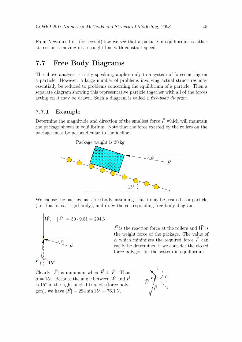
Determine the magnitude and direction of the smallest force ~F which will maintainthe package shown in equilibrium. Note that the force exerted by the rollers on thepackage must be perpendicular to the incline.

��

��

Package weight is 30 kg

15◦

α~F

We choose the package as a free body, assuming that it may be treated as a particle(i.e. that it is a rigid body), and draw the corresponding free body diagram.

~W, | ~W | = 30 · 9.81 = 294 N

α

15◦

~F

~P

~P is the reaction force at the rollers and ~W isthe weight force of the package. The value ofα which minimizes the required force ~F caneasily be determined if we consider the closedforce polygon for the system in equilibrium.

Clearly |~F | is minimum when ~F ⊥ ~P . Thus

α = 15◦. Because the angle between ~W and ~Pis 15◦ in the right angled triangle (force poly-

gon), we have |~F | = 294 sin 15◦ = 76.1 N.

α

~P

~W~F


7.8 Rigid Bodies: Force Equivalents

So far we have neglected the size of the bodies considered and treated them asparticles. When the size of a body is important analysis is still straightforward if itis a rigid body, that is one that does not deform. Actual structures or machines aresubject to small deformations which often do not appreciably affect the conditionsof equilibrium or motion of the structure under consideration. To begin with weshall only be concerned with the external forces applied to the rigid body. Theinternal forces hold the parts (or particles) of the rigid body together, and cancelout by Newton’s third law.

Example

A beam resting on a single pivot, and a free body diagram of the beam showing theexternal forces are shown below.

O OG

d ~S~W

We assume that the weight of the beam may be represented by a single force ~Wacting at a point G, called the centre of gravity of the beam. In the case of a uniformbeam G is located at the midpoint. The downward motion of the beam (due to its

weight) is opposed by the supporting force ~S. Clearly the beam will begin to rotateunless supported at G. W · d measures the tendency of the beam to rotate aboutO in an anticlockwise direction.

7.8.1 Moment

The moment of a force ~F about a point O is defined by

~MO ≡ ~r × ~F

where ~r is the position vector of the point of application A of ~F relative to O.

α

A

O

d

α

~F

~r

From the diagram we see that ~MO ≡ ~r × ~F = ~n |~F | |~r| sin α = ~n F d, where d is the

distance from O to the line of action of ~F , and ~n is a unit vector pointing out ofthe page. Note that | ~MO| = F d, where F = |~F |. The moment of a force in SI unitsis expressed in newton-metres (N · m).


Example

A force of 800 N acts on a bracket as shown. Determine the moment of the forceabout B.

� ��

� ��

200 mm

160 mm

60◦

~i

~jA

B

800 N

The moment about B is ~MB = ~rA/B × ~F , where ~rA/B is the position of A relative

to B, i.e. ~rA/B = −0.2~i + 0.16~j (in metres!). Now

~F = 800 cos 60◦~i + 800 sin 60◦~j = 400~i + 692.8~j N

thus

~MB = (−0.2~i + 0.16~j) × (400~i + 692.8~j)

= −138.56~k − 64~k

= −(203 N · m)~k (3sf).

This is often written as~MB = 203 N · m

7.8.2 Varigon’s Theorem

Consider a force ~R which is the resultant of several concurrent forces (i.e. forces

applied at the same point) ~F1, ~F2, . . ., ~Fn. Then the moment of ~R about any given

point O is equal to the sum of the moments of ~F1 through ~Fn about O.

Proof

Varigon’s theorem is an immediate consequence of the distributive law for the vectorproduct1.

~MO = ~r × ~R

= ~r × (~F1 + ~F2 + . . . + ~Fn)

= ~r × ~F1 + ~r × ~F2 + . . . + ~r × ~Fn

=n

∑

i=1

~M iO

1The proof of the distributive law involves expanding both sides of the equation ~A× ( ~B + ~C) =~A × ~B + ~A × ~C in coordinate form.


7.8.3 Equivalent Forces Theorem

We say that two systems of forces ~F1, ~F2, . . ., ~Fm and ~F ∗1 , ~F ∗

2 , . . ., ~F ∗n acting on a

rigid body are equivalent if and only if both of the following conditions hold:

1. The resultants of the force systems are equal, i.e.m

∑

i=1

~Fi =n

∑

j=1

~F ∗j

2. There is a point O such that the sums of the moments of the two systemsabout O are equal, i.e.

m∑

i=1

~ri × ~Fi =n

∑

j=1

~r∗j × ~F ∗j

The next theorem tells us that O can be any point.

Theorem

If two force systems are equivalent then the two systems must have the same momentabout every point.

Proof

We’ll prove this in the case of two equivalent force systems where all forces areapplied at a point A in the rigid body. Then

∑ ~F =∑ ~F ∗ and there is a point O

such that∑ ~MO =

∑ ~M∗O. We wish to show that for any given point Q we have

∑ ~MQ =∑ ~M∗

Q.

Q

~F1

~F2

~F ∗1A

O~QA

~OA

~OQ

∑

~MO =∑

~OA × ~Fi

=∑

( ~OQ + ~QA) × ~Fi

= ~OQ ×∑

~Fi +∑

~QA × ~Fi

= ~OQ × ~R +∑

~QA × ~Fi

where ~R =∑ ~Fi =

∑ ~F ∗j since the two systems are equivalent. The same process

for the second system gives us∑

~M∗O = ~OQ × ~R +

∑

~QA × ~F ∗j


Thus∑

~QA × ~Fi =∑

~QA × ~F ∗j

proving the theorem for the case of concurrent forces. Proof for the general case,where each force may be applied at a different location, is essentially the same asthis, but requires more notation to account for the various points of application.

7.8.4 Beam Corollary

The weight of a uniform beam of mass M may be represented by a single force~W = −M g~j acting at the centre of gravity G, which is at the centre of the uniformbeam.

mass m.particles, each oflarge number ofBeam regarded as a

Beam regarded as asingle particle ofmass M =

∑

m.

G

m g m g

ydd

M g

x

By symmetry, we see that both force systems have zero moment about the centreG, and

∑

−m g~j = −g~j∑

m = −M g~j = ~W.

Since both force systems have the same sum and moment about G they must be

equivalent ; in other words the two force systems must have the same effect on thebeam.

Date post:	26-Mar-2018
Category:	Documents
Upload:	hoangphuc
View:	216 times
Download:	0 times

Computational Modelling 201 (Numerical Methods)jenlow/files/como201_lectures.pdf · Computational...

Documents