Numerical Optimization for Economists Todd Munson Mathematics and Computer Division Argonne National Laboratory [email protected]Institute for Computational Economics University of Chicago July 19–30, 2010 Munson Numerical Optimization
Institute for Computational EconomicsUniversity of Chicago
July 19–30, 2010
Munson Numerical Optimization
Part I
Numerical Optimization: Introduction
Munson Numerical Optimization
Modeling Language Benefits
• Portable language for optimization problems• Algebraic description• Models easily modified and solved• Large problems can be processed• Programming language features
• Many available optimization algorithms• No need to compile C/FORTRAN code• Derivatives automatically calculated• Algorithms specific options can be set
• Communication with other tools• Relational databases and spreadsheets• MATLAB interface for function evaluations
• Excellent documentation
• Large user communities
Munson Numerical Optimization
Modeling Languages Versus Solver Libraries
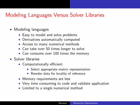
• Modeling languages• Easy to model and solve problems• Derivatives automatically computed• Access to many numerical methods
• Can take over 50 times longer to solve• Can consume over 100 times the memory
• Solver libraries• Computationally efficient
• Select appropriate matrix representation• Reorder data for locality of reference
• Memory requirements are less• Very time consuming to code and validate application• Limited to a single numerical method
Munson Numerical Optimization
Modeling Languages Versus Solver Libraries
• Modeling languages• Easy to model and solve problems• Derivatives automatically computed• Access to many numerical methods• Can take over 50 times longer to solve• Can consume over 100 times the memory
• Solver libraries• Computationally efficient
• Select appropriate matrix representation• Reorder data for locality of reference
• Memory requirements are less
• Very time consuming to code and validate application• Limited to a single numerical method
Munson Numerical Optimization
Modeling Languages Versus Solver Libraries
• Modeling languages• Easy to model and solve problems• Derivatives automatically computed• Access to many numerical methods• Can take over 50 times longer to solve• Can consume over 100 times the memory
• Solver libraries• Computationally efficient
• Select appropriate matrix representation• Reorder data for locality of reference
• Memory requirements are less• Very time consuming to code and validate application• Limited to a single numerical method
Munson Numerical Optimization
Model Declaration
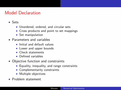
• Sets• Unordered, ordered, and circular sets• Cross products and point to set mappings• Set manipulation
• Parameters and variables• Initial and default values• Lower and upper bounds• Check statements• Defined variables
• Objective function and constraints• Equality, inequality, and range constraints• Complementarity constraints• Multiple objectives
• Problem statement
Munson Numerical Optimization
Data and Commands
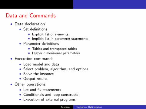
• Data declaration• Set definitions
• Explicit list of elements• Implicit list in parameter statements
• Parameter definitions• Tables and transposed tables• Higher dimensional parameters
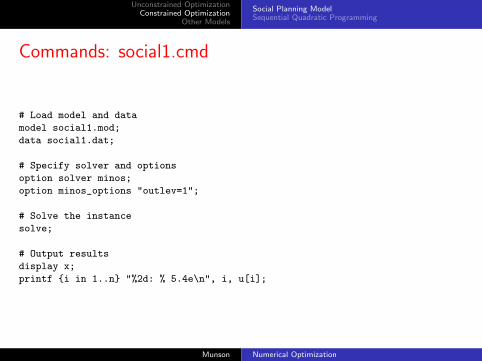
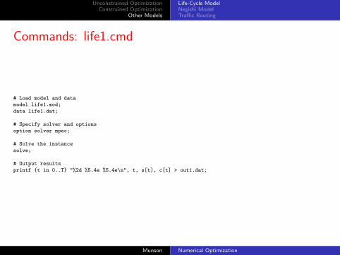
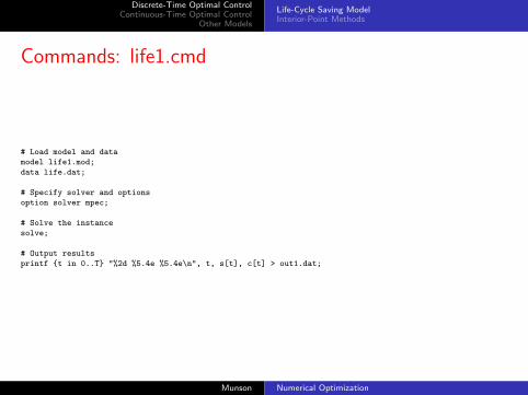
• Execution commands• Load model and data• Select problem, algorithm, and options• Solve the instance• Output results
• Other operations• Let and fix statements• Conditionals and loop constructs• Execution of external programs
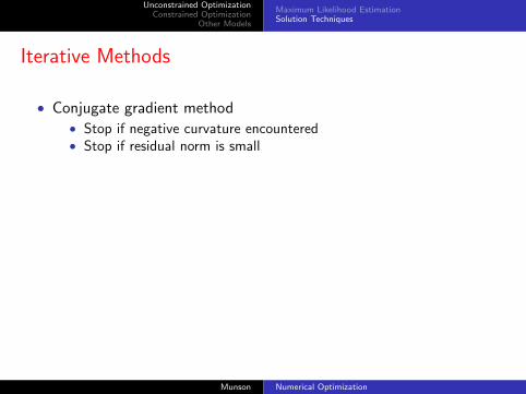
• Conjugate gradient method• Stop if negative curvature encountered• Stop if residual norm is small
• Conjugate gradient method with trust region• Nash
• Follow direction to boundary if first iteration• Stop at base of direction otherwise
• Steihaug-Toint• Follow direction to boundary
• Generalized Lanczos• Compute tridiagonal approximation• Find global solution to approximate problem on boundary• Initialize perturbation with approximate minimum eigenvalue
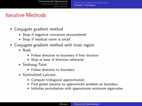
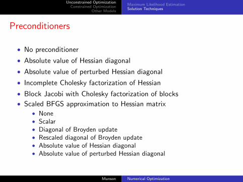
• Block Jacobi with Cholesky factorization of blocks
• Scaled BFGS approximation to Hessian matrix• None• Scalar• Diagonal of Broyden update• Rescaled diagonal of Broyden update• Absolute value of Hessian diagonal• Absolute value of perturbed Hessian diagonal
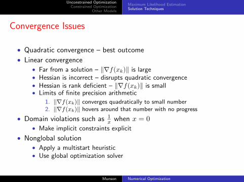
• Linear convergence• Far from a solution – ‖∇f(xk)‖ is large• Hessian is incorrect – disrupts quadratic convergence• Hessian is rank deficient – ‖∇f(xk)‖ is small• Limits of finite precision arithmetic
1. ‖∇f(xk)‖ converges quadratically to small number2. ‖∇f(xk)‖ hovers around that number with no progress
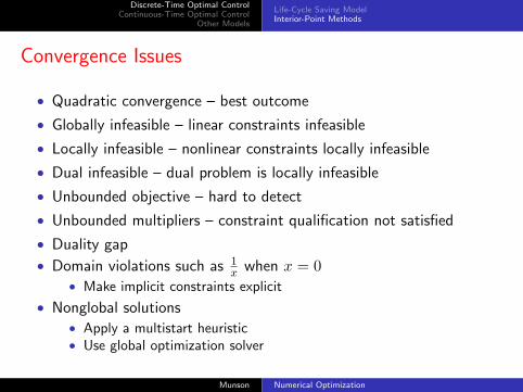
• Domain violations such as 1x when x = 0
• Make implicit constraints explicit
• Nonglobal solution• Apply a multistart heuristic• Use global optimization solver
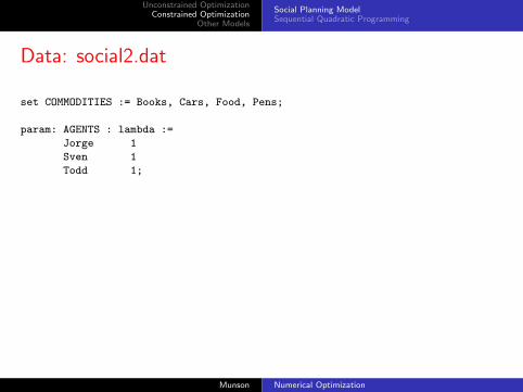
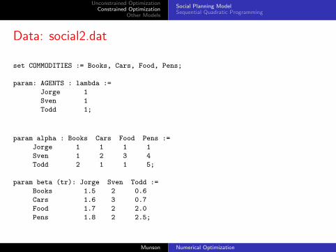
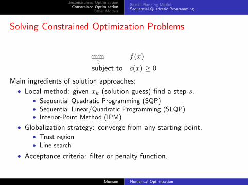
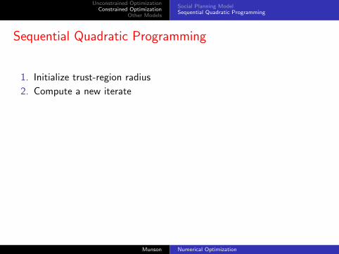
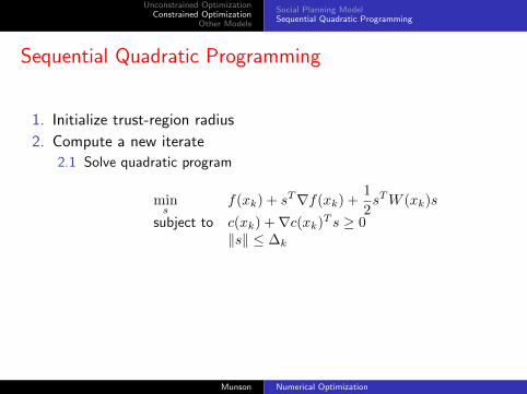
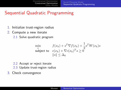
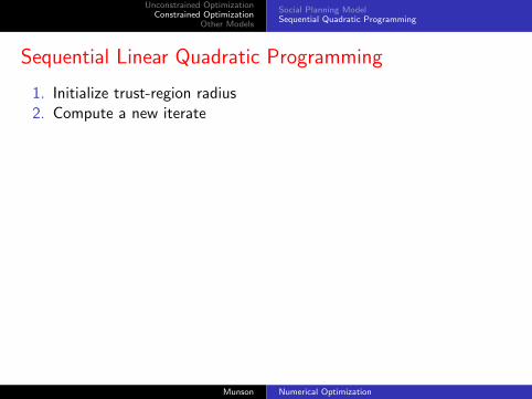
Social Planning ModelSequential Quadratic Programming
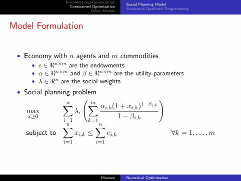
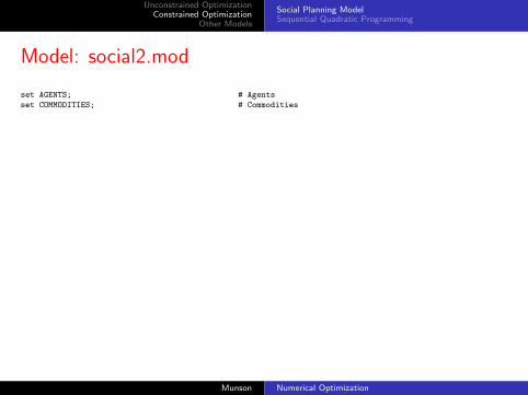
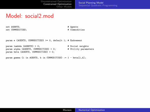
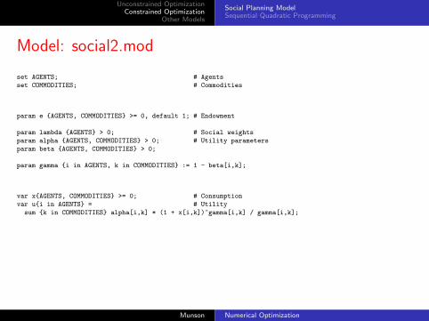
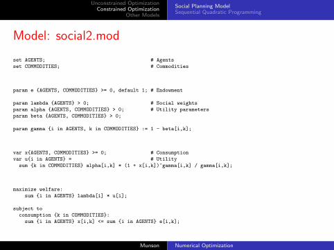
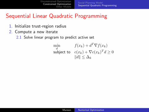
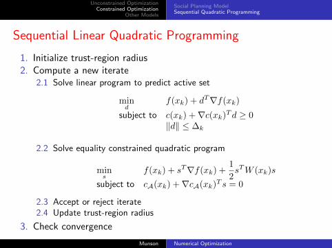
Model Formulation
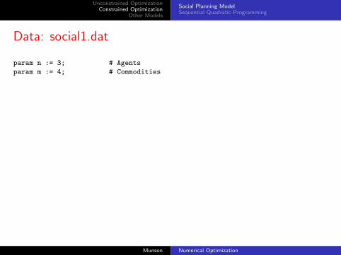
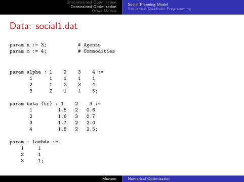
• Economy with n agents and m commodities• e ∈ <n×m are the endowments• α ∈ <n×m and β ∈ <n×m are the utility parameters• λ ∈ <n are the social weights
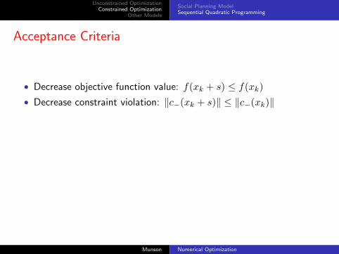
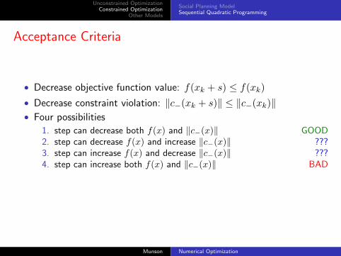
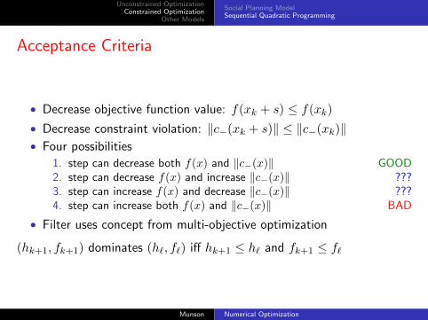
1. step can decrease both f(x) and ‖c−(x)‖ GOOD2. step can decrease f(x) and increase ‖c−(x)‖ ???3. step can increase f(x) and decrease ‖c−(x)‖ ???4. step can increase both f(x) and ‖c−(x)‖ BAD
• Filter uses concept from multi-objective optimization
1. step can decrease both f(x) and ‖c−(x)‖ GOOD2. step can decrease f(x) and increase ‖c−(x)‖ ???3. step can increase f(x) and decrease ‖c−(x)‖ ???4. step can increase both f(x) and ‖c−(x)‖ BAD
• Filter uses concept from multi-objective optimization
1. step can decrease both f(x) and ‖c−(x)‖ GOOD2. step can decrease f(x) and increase ‖c−(x)‖ ???3. step can increase f(x) and decrease ‖c−(x)‖ ???4. step can increase both f(x) and ‖c−(x)‖ BAD
• Filter uses concept from multi-objective optimization
Social Planning ModelSequential Quadratic Programming
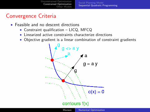
Convergence Criteria
• Feasible and no descent directions• Constraint qualification – LICQ, MFCQ• Linearized active constraints characterize directions• Objective gradient is a linear combination of constraint gradients
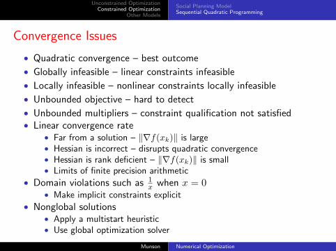
• Unbounded multipliers – constraint qualification not satisfied• Linear convergence rate
• Far from a solution – ‖∇f(xk)‖ is large• Hessian is incorrect – disrupts quadratic convergence• Hessian is rank deficient – ‖∇f(xk)‖ is small• Limits of finite precision arithmetic
• Domain violations such as 1x when x = 0
• Make implicit constraints explicit
• Nonglobal solutions• Apply a multistart heuristic• Use global optimization solver
• Maximize discounted utility• u(·) is the utility function• R is the retirement age• T is the terminal age• w is the wage• β is the discount factor• r is the interest rate
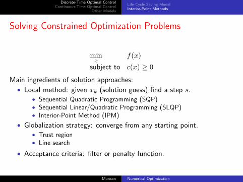
• Optimization problem
maxs,c
T∑t=0
βtu(ct)
subject to st+1 = (1 + r)st + w − ct t = 0, . . . , R− 1st+1 = (1 + r)st − ct t = R, . . . , Ts0 = sT+1 = 0
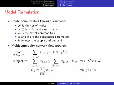
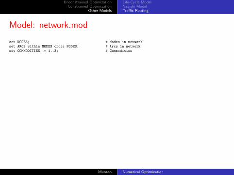
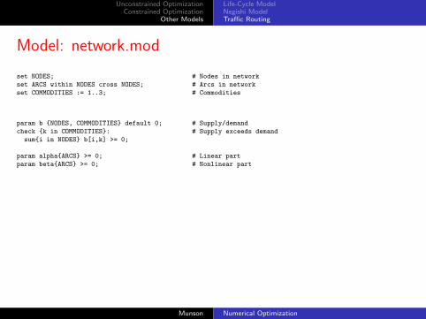
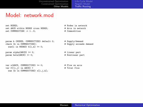
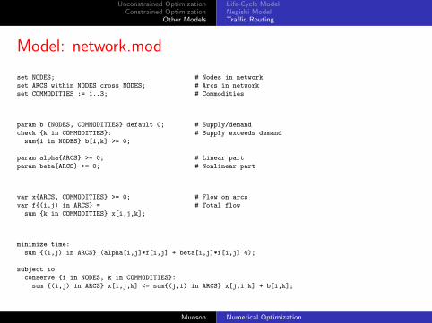
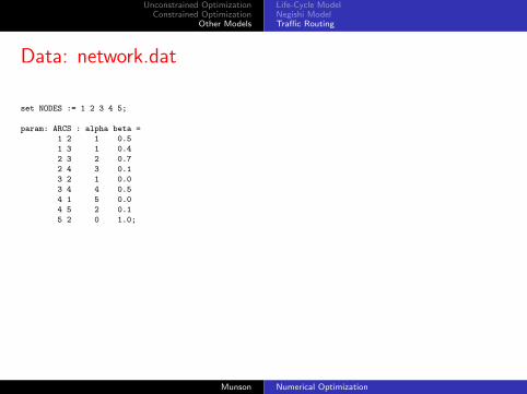
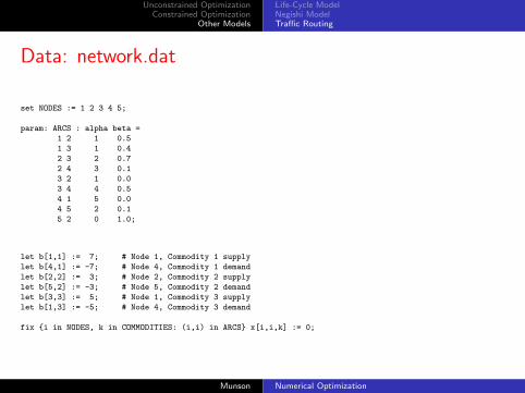
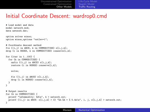
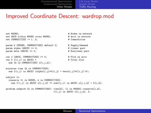
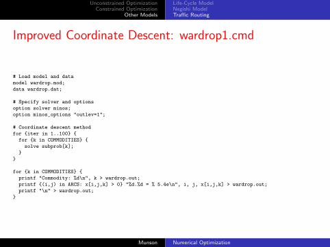
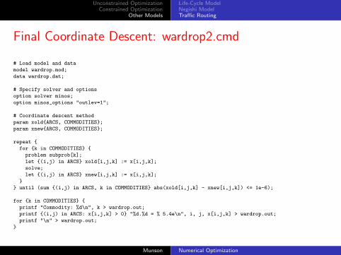
• Route commodities through a network• N is the set of nodes• A ⊆ N ×N is the set of arcs• K is the set of commodities• α and β are the congestion parameters• b denotes the supply and demand
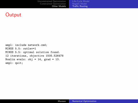
} until (sum {(i,j) in ARCS, k in COMMODITIES} abs(xold[i,j,k] - xnew[i,j,k]) <= 1e-6);
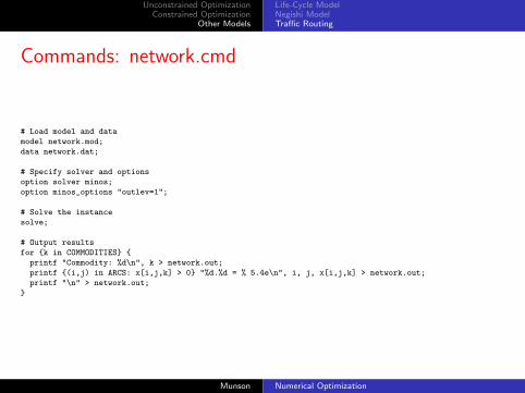
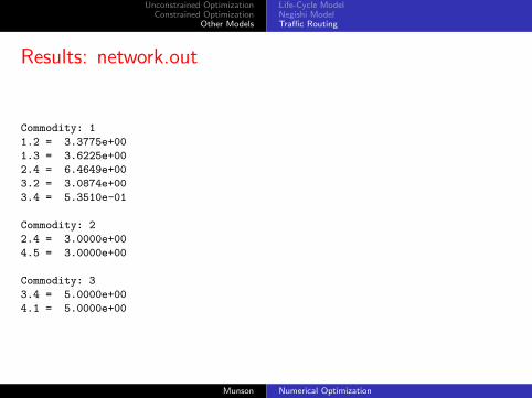
for {k in COMMODITIES} {
printf "Commodity: %d\n", k > wardrop.out;
printf {(i,j) in ARCS: x[i,j,k] > 0} "%d.%d = % 5.4e\n", i, j, x[i,j,k] > wardrop.out;
printf "\n" > wardrop.out;
}
Munson Numerical Optimization
Discrete-Time Optimal ControlContinuous-Time Optimal Control
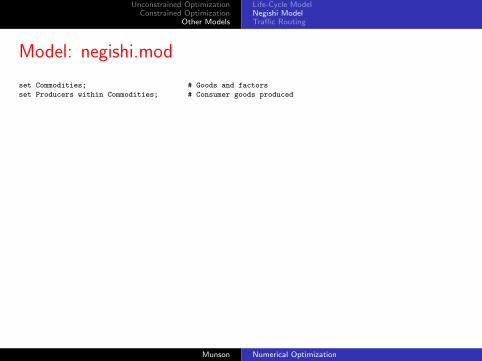
Other Models
Part III
Numerical Optimization II: Optimal Control
Munson Numerical Optimization
Discrete-Time Optimal ControlContinuous-Time Optimal Control
Other Models
Life-Cycle Saving ModelInterior-Point Methods
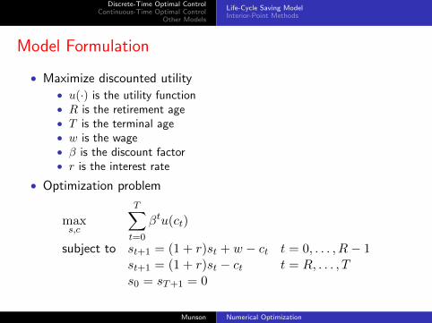
Model Formulation
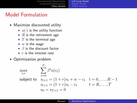
• Maximize discounted utility• u(·) is the utility function• R is the retirement age• T is the terminal age• w is the wage• β is the discount factor• r is the interest rate
• Optimization problem
maxs,c
T∑t=0
βtu(ct)
subject to st+1 = (1 + r)st + w − ct t = 0, . . . , R− 1st+1 = (1 + r)st − ct t = R, . . . , Ts0 = sT+1 = 0
Munson Numerical Optimization
Discrete-Time Optimal ControlContinuous-Time Optimal Control
Other Models
Life-Cycle Saving ModelInterior-Point Methods
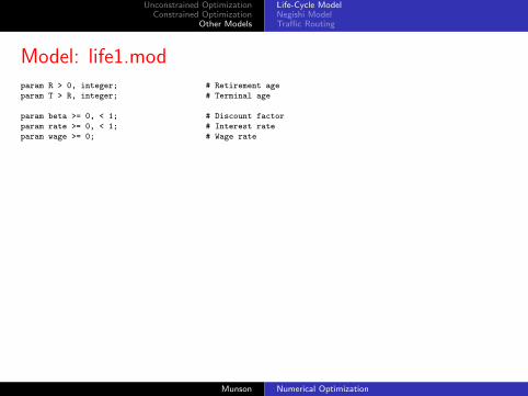
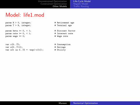
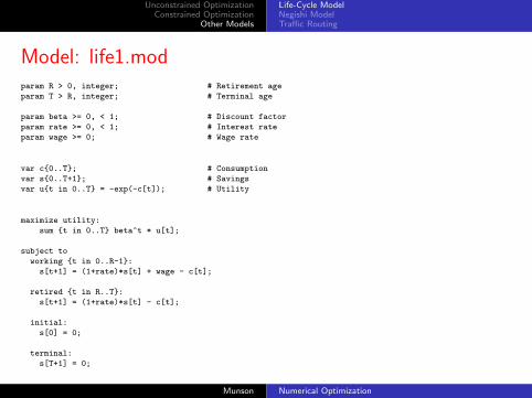
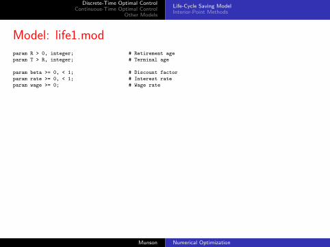
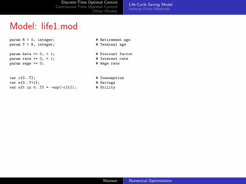
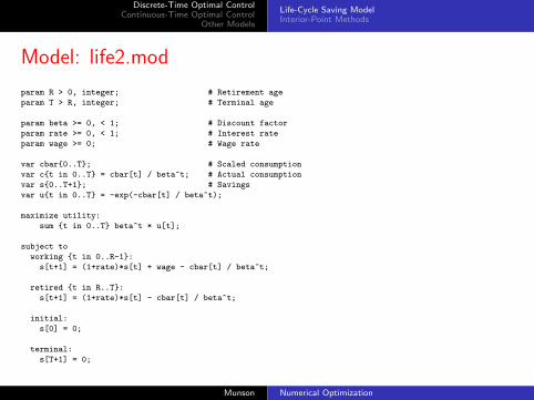
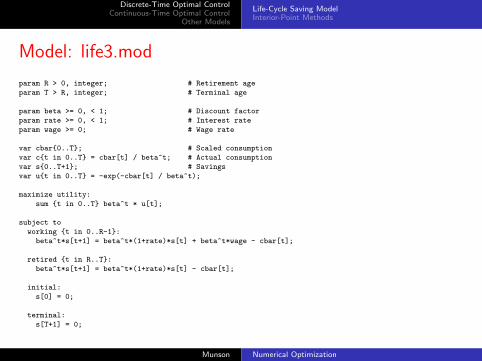
Model: life1.modparam R > 0, integer; # Retirement age
param T > R, integer; # Terminal age
param beta >= 0, < 1; # Discount factor
param rate >= 0, < 1; # Interest rate
param wage >= 0; # Wage rate
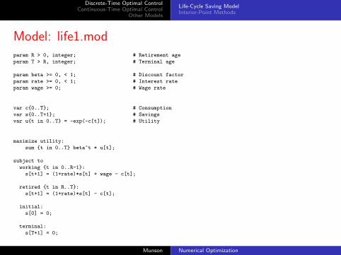
var c{0..T}; # Consumption
var s{0..T+1}; # Savings
var u{t in 0..T} = -exp(-c[t]); # Utility
maximize utility:
sum {t in 0..T} beta^t * u[t];
subject to
working {t in 0..R-1}:
s[t+1] = (1+rate)*s[t] + wage - c[t];
retired {t in R..T}:
s[t+1] = (1+rate)*s[t] - c[t];
initial:
s[0] = 0;
terminal:
s[T+1] = 0;
Munson Numerical Optimization
Discrete-Time Optimal ControlContinuous-Time Optimal Control
Other Models
Life-Cycle Saving ModelInterior-Point Methods
Model: life1.modparam R > 0, integer; # Retirement age
param T > R, integer; # Terminal age
param beta >= 0, < 1; # Discount factor
param rate >= 0, < 1; # Interest rate
param wage >= 0; # Wage rate
var c{0..T}; # Consumption
var s{0..T+1}; # Savings
var u{t in 0..T} = -exp(-c[t]); # Utility
maximize utility:
sum {t in 0..T} beta^t * u[t];
subject to
working {t in 0..R-1}:
s[t+1] = (1+rate)*s[t] + wage - c[t];
retired {t in R..T}:
s[t+1] = (1+rate)*s[t] - c[t];
initial:
s[0] = 0;
terminal:
s[T+1] = 0;
Munson Numerical Optimization
Discrete-Time Optimal ControlContinuous-Time Optimal Control
Other Models
Life-Cycle Saving ModelInterior-Point Methods
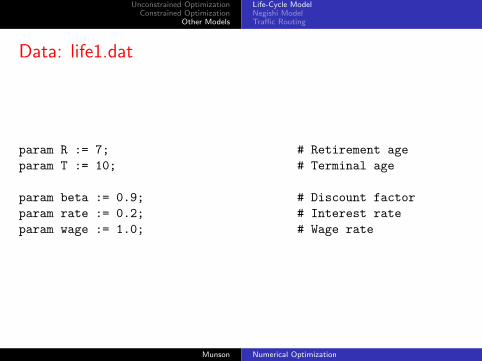
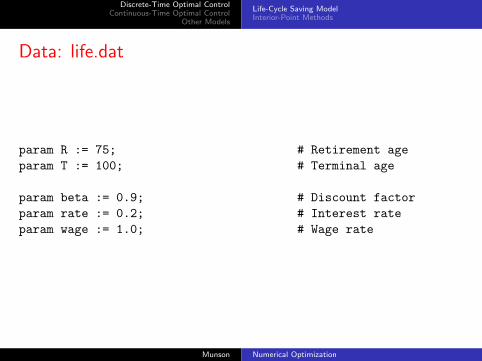
Data: life.dat
param R := 75; # Retirement age
param T := 100; # Terminal age
param beta := 0.9; # Discount factor
param rate := 0.2; # Interest rate
param wage := 1.0; # Wage rate
Munson Numerical Optimization
Discrete-Time Optimal ControlContinuous-Time Optimal Control
Complementarity ProblemsMathematical Programs with Equilibrium Constraints
Other Models
Arrow-Debreu ModelGeneralized Newton Methods
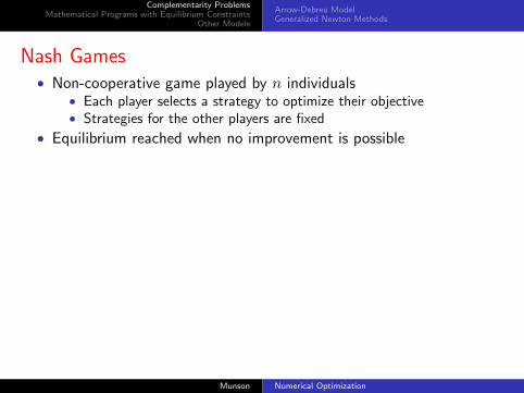
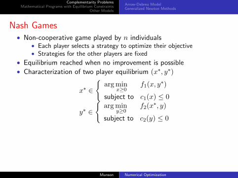
Nash Games• Non-cooperative game played by n individuals
• Each player selects a strategy to optimize their objective• Strategies for the other players are fixed
• Equilibrium reached when no improvement is possible
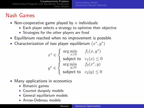
• Characterization of two player equilibrium (x∗, y∗)
x∗ ∈
{arg min
x≥0f1(x, y
∗)
subject to c1(x) ≤ 0
y∗ ∈
{arg min
y≥0f2(x
∗, y)
subject to c2(y) ≤ 0
• Many applications in economics• Bimatrix games• Cournot duopoly models• General equilibrium models• Arrow-Debreau models
Munson Numerical Optimization
Complementarity ProblemsMathematical Programs with Equilibrium Constraints
Other Models
Arrow-Debreu ModelGeneralized Newton Methods
Nash Games• Non-cooperative game played by n individuals
• Each player selects a strategy to optimize their objective• Strategies for the other players are fixed
• Equilibrium reached when no improvement is possible• Characterization of two player equilibrium (x∗, y∗)
x∗ ∈
{arg min
x≥0f1(x, y
∗)
subject to c1(x) ≤ 0
y∗ ∈
{arg min
y≥0f2(x
∗, y)
subject to c2(y) ≤ 0
• Many applications in economics• Bimatrix games• Cournot duopoly models• General equilibrium models• Arrow-Debreau models
Munson Numerical Optimization
Complementarity ProblemsMathematical Programs with Equilibrium Constraints
Other Models
Arrow-Debreu ModelGeneralized Newton Methods
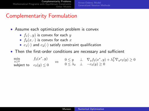
Complementarity Formulation
• Assume each optimization problem is convex• f1(·, y) is convex for each y• f2(x, ·) is convex for each x• c1(·) and c2(·) satisfy constraint qualification
• Then the first-order conditions are necessary and sufficient
minx≥0
f1(x, y∗)
subject to c1(x) ≤ 0⇔ 0 ≤ x ⊥ ∇xf1(x, y
∗) + λT1∇xc1(x) ≥ 0
0 ≤ λ1 ⊥ −c1(x) ≥ 0
Munson Numerical Optimization
Complementarity ProblemsMathematical Programs with Equilibrium Constraints
Other Models
Arrow-Debreu ModelGeneralized Newton Methods
Complementarity Formulation
• Assume each optimization problem is convex• f1(·, y) is convex for each y• f2(x, ·) is convex for each x• c1(·) and c2(·) satisfy constraint qualification
• Then the first-order conditions are necessary and sufficient
miny≥0
f2(x∗, y)
subject to c2(y) ≤ 0⇔ 0 ≤ y ⊥ ∇yf2(x
∗, y) + λT2∇yc2(y) ≥ 0
0 ≤ λ2 ⊥ −c2(y) ≥ 0
Munson Numerical Optimization
Complementarity ProblemsMathematical Programs with Equilibrium Constraints
Other Models
Arrow-Debreu ModelGeneralized Newton Methods
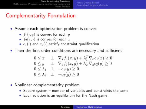
Complementarity Formulation
• Assume each optimization problem is convex• f1(·, y) is convex for each y• f2(x, ·) is convex for each x• c1(·) and c2(·) satisfy constraint qualification
• Then the first-order conditions are necessary and sufficient
• Nonlinear complementarity problem• Square system – number of variables and constraints the same• Each solution is an equilibrium for the Nash game
Munson Numerical Optimization
Complementarity ProblemsMathematical Programs with Equilibrium Constraints
Other Models
Arrow-Debreu ModelGeneralized Newton Methods
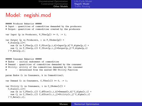
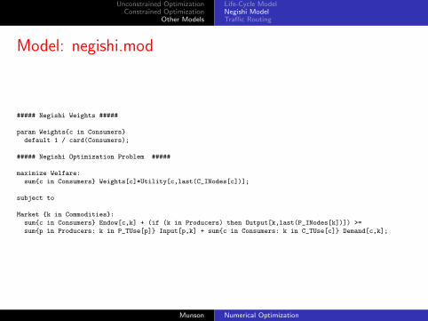
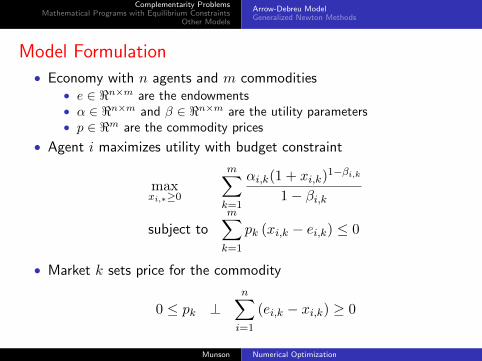
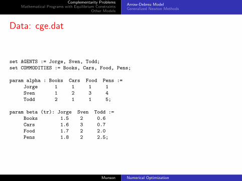
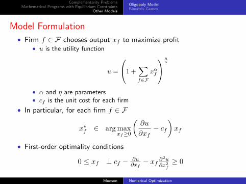
Model Formulation
• Economy with n agents and m commodities• e ∈ <n×m are the endowments• α ∈ <n×m and β ∈ <n×m are the utility parameters• p ∈ <m are the commodity prices
• Agent i maximizes utility with budget constraint
maxxi,∗≥0
m∑k=1
αi,k(1 + xi,k)1−βi,k
1− βi,k
subject tom∑k=1
pk (xi,k − ei,k) ≤ 0
• Market k sets price for the commodity
0 ≤ pk ⊥n∑i=1
(ei,k − xi,k) ≥ 0
Munson Numerical Optimization
Complementarity ProblemsMathematical Programs with Equilibrium Constraints
Other Models
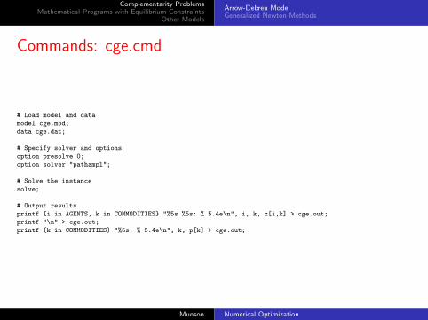
Arrow-Debreu ModelGeneralized Newton Methods
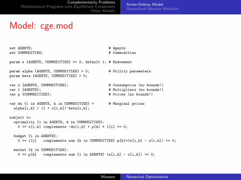
Model: cge.mod
set AGENTS; # Agents
set COMMODITIES; # Commodities
param e {AGENTS, COMMODITIES} >= 0, default 1; # Endowment
Complementarity ProblemsMathematical Programs with Equilibrium Constraints
Other Models
Arrow-Debreu ModelGeneralized Newton Methods
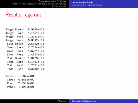
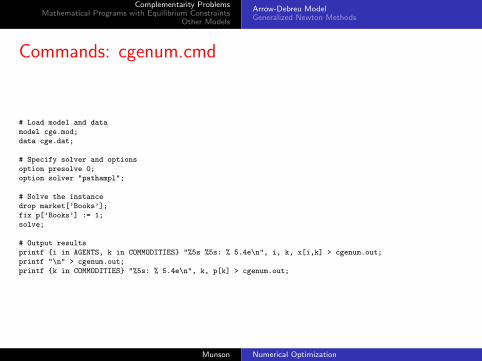
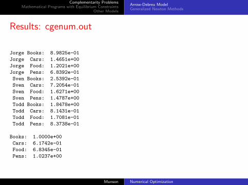
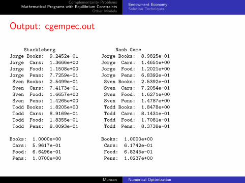
Results: cgenum.out
Jorge Books: 8.9825e-01
Jorge Cars: 1.4651e+00
Jorge Food: 1.2021e+00
Jorge Pens: 6.8392e-01
Sven Books: 2.5392e-01
Sven Cars: 7.2054e-01
Sven Food: 1.6271e+00
Sven Pens: 1.4787e+00
Todd Books: 1.8478e+00
Todd Cars: 8.1431e-01
Todd Food: 1.7081e-01
Todd Pens: 8.3738e-01
Books: 1.0000e+00
Cars: 6.1742e-01
Food: 6.8345e-01
Pens: 1.0237e+00
Munson Numerical Optimization
Complementarity ProblemsMathematical Programs with Equilibrium Constraints
Other Models
Arrow-Debreu ModelGeneralized Newton Methods
Pitfalls
• Nonsquare systems• Side variables• Side constraints
• Orientation of equations• Skew symmetry preferred• Proximal point perturbation
• AMPL presolve• option presolve 0;
Munson Numerical Optimization
Complementarity ProblemsMathematical Programs with Equilibrium Constraints
Other Models
Arrow-Debreu ModelGeneralized Newton Methods
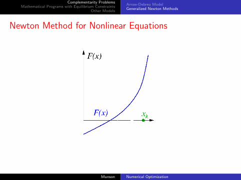
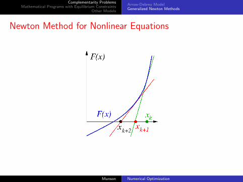
Newton Method for Nonlinear Equations
Munson Numerical Optimization
Complementarity ProblemsMathematical Programs with Equilibrium Constraints
Other Models
Arrow-Debreu ModelGeneralized Newton Methods
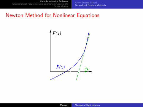
Newton Method for Nonlinear Equations
Munson Numerical Optimization
Complementarity ProblemsMathematical Programs with Equilibrium Constraints
Other Models
Arrow-Debreu ModelGeneralized Newton Methods
Newton Method for Nonlinear Equations
Munson Numerical Optimization
Complementarity ProblemsMathematical Programs with Equilibrium Constraints
Other Models
Arrow-Debreu ModelGeneralized Newton Methods
Newton Method for Nonlinear Equations
Munson Numerical Optimization
Complementarity ProblemsMathematical Programs with Equilibrium Constraints
Other Models
Arrow-Debreu ModelGeneralized Newton Methods
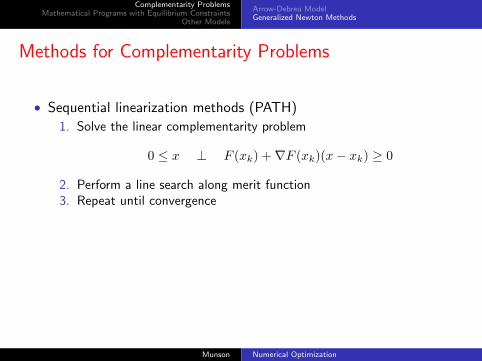
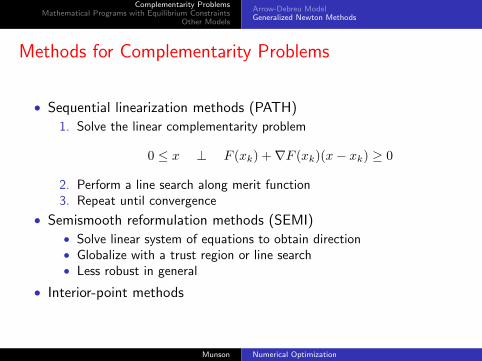
Methods for Complementarity Problems
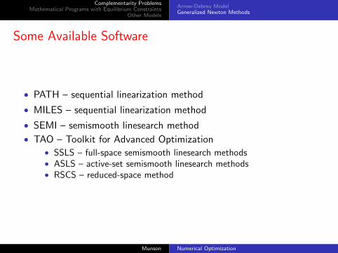
• Sequential linearization methods (PATH)
1. Solve the linear complementarity problem
0 ≤ x ⊥ F (xk) +∇F (xk)(x− xk) ≥ 0
2. Perform a line search along merit function3. Repeat until convergence
• Semismooth reformulation methods (SEMI)• Solve linear system of equations to obtain direction• Globalize with a trust region or line search• Less robust in general
• Interior-point methods
Munson Numerical Optimization
Complementarity ProblemsMathematical Programs with Equilibrium Constraints
Other Models
Arrow-Debreu ModelGeneralized Newton Methods
Methods for Complementarity Problems
• Sequential linearization methods (PATH)
1. Solve the linear complementarity problem
0 ≤ x ⊥ F (xk) +∇F (xk)(x− xk) ≥ 0
2. Perform a line search along merit function3. Repeat until convergence
• Semismooth reformulation methods (SEMI)• Solve linear system of equations to obtain direction• Globalize with a trust region or line search• Less robust in general
• Interior-point methods
Munson Numerical Optimization
Complementarity ProblemsMathematical Programs with Equilibrium Constraints
Other Models
Arrow-Debreu ModelGeneralized Newton Methods
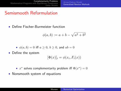
Semismooth Reformulation
• Define Fischer-Burmeister function
φ(a, b) := a+ b−√a2 + b2
• φ(a, b) = 0 iff a ≥ 0, b ≥ 0, and ab = 0
• Define the system[Φ(x)]i = φ(xi, Fi(x))
• x∗ solves complementarity problem iff Φ(x∗) = 0
• Nonsmooth system of equations
Munson Numerical Optimization
Complementarity ProblemsMathematical Programs with Equilibrium Constraints
Other Models
Arrow-Debreu ModelGeneralized Newton Methods
Semismooth Algorithm
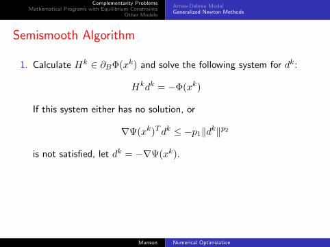
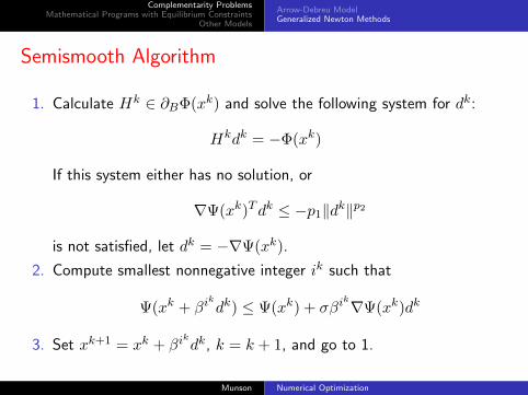
1. Calculate Hk ∈ ∂BΦ(xk) and solve the following system for dk:
Hkdk = −Φ(xk)
If this system either has no solution, or
∇Ψ(xk)Tdk ≤ −p1‖dk‖p2
is not satisfied, let dk = −∇Ψ(xk).
2. Compute smallest nonnegative integer ik such that
Ψ(xk + βikdk) ≤ Ψ(xk) + σβi
k∇Ψ(xk)dk
3. Set xk+1 = xk + βikdk, k = k + 1, and go to 1.
Munson Numerical Optimization
Complementarity ProblemsMathematical Programs with Equilibrium Constraints
Other Models
Arrow-Debreu ModelGeneralized Newton Methods
Semismooth Algorithm
1. Calculate Hk ∈ ∂BΦ(xk) and solve the following system for dk:
Hkdk = −Φ(xk)
If this system either has no solution, or
∇Ψ(xk)Tdk ≤ −p1‖dk‖p2
is not satisfied, let dk = −∇Ψ(xk).
2. Compute smallest nonnegative integer ik such that
Ψ(xk + βikdk) ≤ Ψ(xk) + σβi
k∇Ψ(xk)dk
3. Set xk+1 = xk + βikdk, k = k + 1, and go to 1.
Munson Numerical Optimization
Complementarity ProblemsMathematical Programs with Equilibrium Constraints
Other Models
Arrow-Debreu ModelGeneralized Newton Methods
Convergence Issues
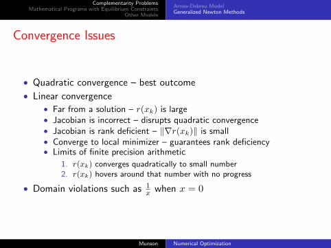
• Quadratic convergence – best outcome
• Linear convergence• Far from a solution – r(xk) is large• Jacobian is incorrect – disrupts quadratic convergence• Jacobian is rank deficient – ‖∇r(xk)‖ is small• Converge to local minimizer – guarantees rank deficiency• Limits of finite precision arithmetic
1. r(xk) converges quadratically to small number2. r(xk) hovers around that number with no progress
• Domain violations such as 1x when x = 0
Munson Numerical Optimization
Complementarity ProblemsMathematical Programs with Equilibrium Constraints
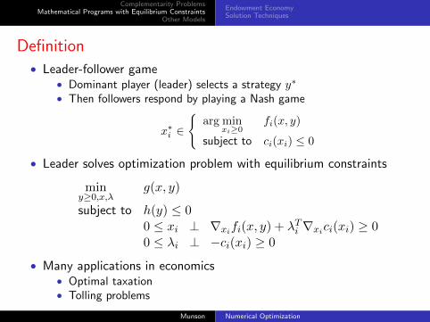
• Many applications in economics• Optimal taxation• Tolling problems
Munson Numerical Optimization
Complementarity ProblemsMathematical Programs with Equilibrium Constraints
Other Models
Endowment EconomySolution Techniques
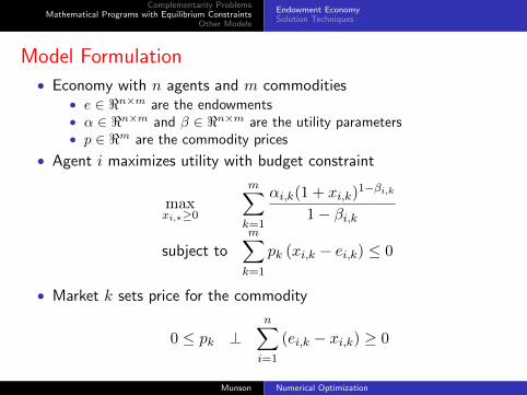
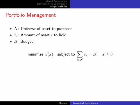
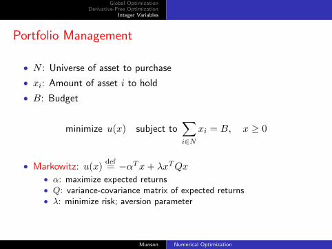
Model Formulation
• Economy with n agents and m commodities• e ∈ <n×m are the endowments• α ∈ <n×m and β ∈ <n×m are the utility parameters• p ∈ <m are the commodity prices
• Agent i maximizes utility with budget constraint
maxxi,∗≥0
m∑k=1
αi,k(1 + xi,k)1−βi,k
1− βi,k
subject tom∑k=1
pk (xi,k − ei,k) ≤ 0
• Market k sets price for the commodity
0 ≤ pk ⊥n∑i=1
(ei,k − xi,k) ≥ 0
Munson Numerical Optimization
Complementarity ProblemsMathematical Programs with Equilibrium Constraints
Other Models
Endowment EconomySolution Techniques
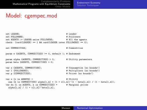
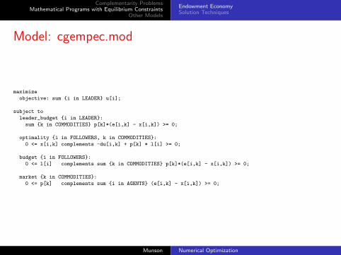
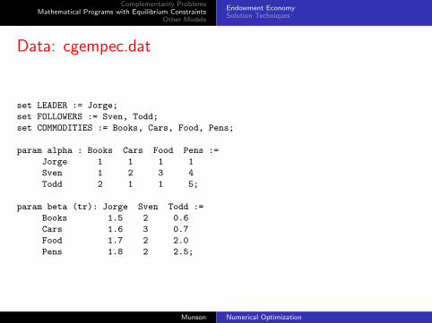
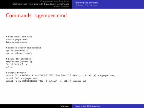
Model: cgempec.mod
set LEADER; # Leader
set FOLLOWERS; # Followers
set AGENTS := LEADER union FOLLOWERS; # All the agents
check: (card(LEADER) == 1 && card(LEADER inter FOLLOWERS) == 0);
set COMMODITIES; # Commodities
param e {AGENTS, COMMODITIES} >= 0, default 1; # Endowment
Complementarity ProblemsMathematical Programs with Equilibrium Constraints
Other Models
Oligopoly ModelBimatrix Games
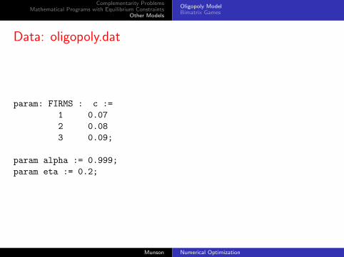
Data: oligopoly.dat
param: FIRMS : c :=
1 0.07
2 0.08
3 0.09;
param alpha := 0.999;
param eta := 0.2;
Munson Numerical Optimization
Complementarity ProblemsMathematical Programs with Equilibrium Constraints
Other Models
Oligopoly ModelBimatrix Games
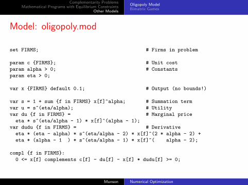
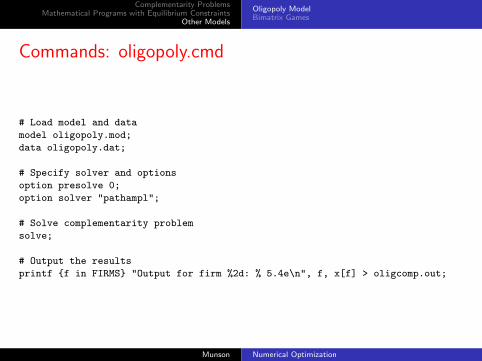
Commands: oligopoly.cmd
# Load model and data
model oligopoly.mod;
data oligopoly.dat;
# Specify solver and options
option presolve 0;
option solver "pathampl";
# Solve complementarity problem
solve;
# Output the results
printf {f in FIRMS} "Output for firm %2d: % 5.4e\n", f, x[f] > oligcomp.out;
Munson Numerical Optimization
Complementarity ProblemsMathematical Programs with Equilibrium Constraints
Other Models
Oligopoly ModelBimatrix Games
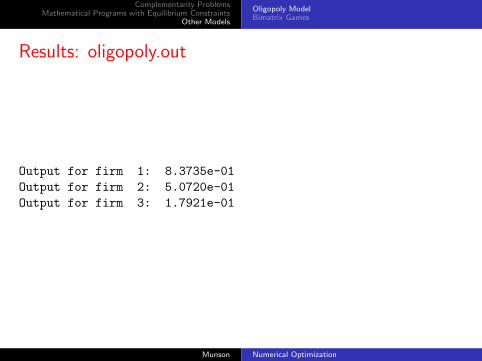
Results: oligopoly.out
Output for firm 1: 8.3735e-01
Output for firm 2: 5.0720e-01
Output for firm 3: 1.7921e-01
Munson Numerical Optimization
Complementarity ProblemsMathematical Programs with Equilibrium Constraints
Other Models
Oligopoly ModelBimatrix Games
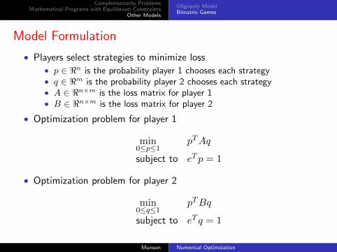
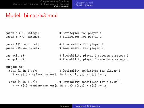
Model Formulation
• Players select strategies to minimize loss• p ∈ <n is the probability player 1 chooses each strategy• q ∈ <m is the probability player 2 chooses each strategy• A ∈ <n×m is the loss matrix for player 1• B ∈ <n×m is the loss matrix for player 2
• Optimization problem for player 1
min0≤p≤1
pTAq
subject to eT p = 1
• Optimization problem for player 2
min0≤q≤1
pTBq
subject to eT q = 1
Munson Numerical Optimization
Complementarity ProblemsMathematical Programs with Equilibrium Constraints
Other Models
Oligopoly ModelBimatrix Games
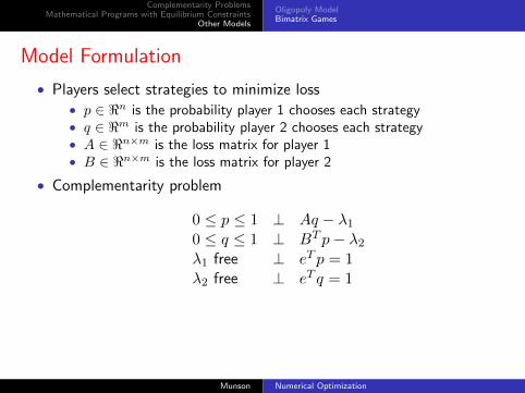
Model Formulation
• Players select strategies to minimize loss• p ∈ <n is the probability player 1 chooses each strategy• q ∈ <m is the probability player 2 chooses each strategy• A ∈ <n×m is the loss matrix for player 1• B ∈ <n×m is the loss matrix for player 2
• Complementarity problem
0 ≤ p ≤ 1 ⊥ Aq − λ10 ≤ q ≤ 1 ⊥ BT p− λ2λ1 free ⊥ eT p = 1λ2 free ⊥ eT q = 1
Munson Numerical Optimization
Complementarity ProblemsMathematical Programs with Equilibrium Constraints
Other Models
Oligopoly ModelBimatrix Games
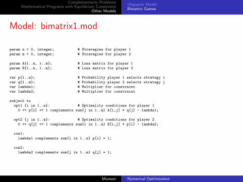
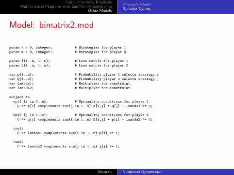
Model: bimatrix1.mod
param n > 0, integer; # Strategies for player 1
param m > 0, integer; # Strategies for player 2
param A{1..n, 1..m}; # Loss matrix for player 1
param B{1..n, 1..m}; # Loss matrix for player 2
var p{1..n}; # Probability player 1 selects strategy i
var q{1..m}; # Probability player 2 selects strategy j
var lambda1; # Multiplier for constraint
var lambda2; # Multiplier for constraint
subject to
opt1 {i in 1..n}: # Optimality conditions for player 1
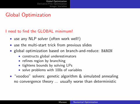
• global optimization based on branch-and-reduce: BARON
• constructs global underestimators• refines region by branching• tightens bounds by solving LPs• solve problems with 100s of variables
• “voodoo” solvers: genetic algorithm & simulated annealingno convergence theory ... usually worse than deterministic
Munson Numerical Optimization
Global OptimizationDerivative-Free Optimization
Integer Variables
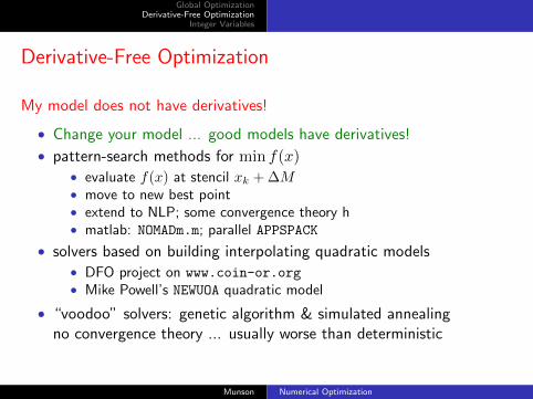
Derivative-Free Optimization
My model does not have derivatives!
• Change your model ... good models have derivatives!
• pattern-search methods for min f(x)• evaluate f(x) at stencil xk + ∆M• move to new best point• extend to NLP; some convergence theory h• matlab: NOMADm.m; parallel APPSPACK
• solvers based on building interpolating quadratic models• DFO project on www.coin-or.org• Mike Powell’s NEWUOA quadratic model
• “voodoo” solvers: genetic algorithm & simulated annealingno convergence theory ... usually worse than deterministic
Munson Numerical Optimization
Global OptimizationDerivative-Free Optimization
Integer Variables
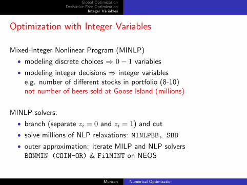
Optimization with Integer Variables
Mixed-Integer Nonlinear Program (MINLP)
• modeling discrete choices ⇒ 0− 1 variables
• modeling integer decisions ⇒ integer variablese.g. number of different stocks in portfolio (8-10)not number of beers sold at Goose Island (millions)
MINLP solvers:
• branch (separate zi = 0 and zi = 1) and cut
• solve millions of NLP relaxations: MINLPBB, SBB
• outer approximation: iterate MILP and NLP solversBONMIN (COIN-OR) & FilMINT on NEOS
• Limit Names: |i ∈ N : xi > 0| ≤ K• Use binary indicator variables to model the implicationxi > 0⇒ yi = 1
• Implication modeled with variable upper bounds:
xi ≤ Byi ∀i ∈ N
•∑i∈N yi ≤ K
Munson Numerical Optimization
Global OptimizationDerivative-Free Optimization
Integer Variables
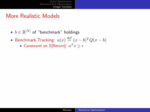
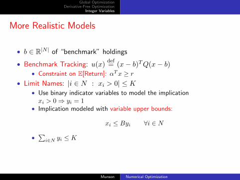
More Realistic Models
• b ∈ R|N | of “benchmark” holdings
• Benchmark Tracking: u(x)def= (x− b)TQ(x− b)
• Constraint on E[Return]: αTx ≥ r• Limit Names: |i ∈ N : xi > 0| ≤ K
• Use binary indicator variables to model the implicationxi > 0⇒ yi = 1
• Implication modeled with variable upper bounds:
xi ≤ Byi ∀i ∈ N
•∑i∈N yi ≤ K
Munson Numerical Optimization
Global OptimizationDerivative-Free Optimization
Integer Variables
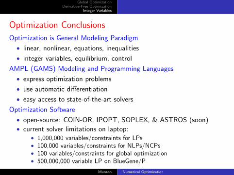
Optimization Conclusions
Optimization is General Modeling Paradigm
• linear, nonlinear, equations, inequalities
• integer variables, equilibrium, control
AMPL (GAMS) Modeling and Programming Languages
• express optimization problems
• use automatic differentiation
• easy access to state-of-the-art solvers
Optimization Software
• open-source: COIN-OR, IPOPT, SOPLEX, & ASTROS (soon)• current solver limitations on laptop:
• 1,000,000 variables/constraints for LPs• 100,000 variables/constraints for NLPs/NCPs• 100 variables/constraints for global optimization• 500,000,000 variable LP on BlueGene/P