Multidisciplinary Simulation, Estimation, and Assimilation Systems Reports in Ocean Science and Engineering MSEAS-11 Numerical Schemes and Computational Studies for Dynamically Orthogonal Equations by Mattheus P. Ueckermann Pierre F. J. Lermusiaux Themis P. Sapsis Department of Mechanical Engineering Massachusetts Institute of Technology Cambridge, Massachusetts August 2011
Transcript
Multidisciplinary Simulation, Estimation, and Assimilation Systems
Reports in Ocean Science and Engineering
MSEAS-11
Numerical Schemes and Computational Studies for Dynamically Orthogonal Equations
by
Mattheus P. Ueckermann Pierre F. J. Lermusiaux
Themis P. Sapsis
Department of Mechanical Engineering Massachusetts Institute of Technology
Cambridge, Massachusetts
August 2011
Numerical Schemes and Computational Studies for Dynamically
Orthogonal Equations
M. P. Ueckermanna, P. F. J. Lermusiauxa, T. P. Sapsis a
aDepartment of Mechanical Engineering, Massachusetts Institute of Technology, 77 Mass. Avenue,Cambridge, MA 02139. Tel.: +1-617-324-5172,
Methods, Total Variation Diminishing, Error Subspace Statistical Estimation, Ocean Modeling, Data
Assimilation
1. Introduction
Quantifying uncertainty is becoming increasingly important in many scientific and engi-neering applications. This is in part because the accuracy of an answer is now often as criticalas the answer itself. Our present motivation is uncertainty prediction for computational fluiddynamics (CFD) applications, specifically in the context of realistic ocean predictions. Inocean dynamics, it is challenging to model multi-scale, intermittent, non-stationary andnon-homogeneous uncertainties. Already a single evaluation of an ocean model is costly andstraightforward stochastic modeling methods are prohibitively expensive [36, 46], particularly
Reports in Ocean Science and Engineering 11 2011
when dealing with longer-term unsteady nonlinear dynamics. Fortunately, the recently de-veloped Dynamically Orthogonal (DO) field equations [50, 49, 51] provide efficient, tractableequations for uncertainty prediction in large-scale CFD and ocean applications. While theseDO equations have been solved numerically using a simple finite-difference scheme, the spe-cific properties of the DO equations warrant novel integration and discretization schemes.Hence, our present goals are to derive efficient computational schemes for the DO methodol-ogy applied to unsteady stochastic Navier-Stokes and Boussinesq dynamics, and to illustrateand study the numerical aspects of these schemes. While we are specifically focused onincompressible fluid flows, the use of generalized inversion to deal with singular subspacecovariances or deterministic modes, and schemes to maintain orthonormal modes at thenumerical level are relevant to any system solved using the DO method.
Stochastic modeling approaches can be categorized as either non-intrusive or intrusive.Non-intrusive approaches have the advantage that the deterministic version of a model canbe used to generate an ensemble of sample solutions from which the statistics can be cal-culated. The disadvantage is that a large number of samples are often required, leading tolarge computational costs. Intrusive approaches require the update of existing codes or thedevelopment of a new code, where the resulting system of equations can be larger than theoriginal, deterministic system. However, intrusive methods are usually computationally lessexpensive than non-intrusive methods, and the statistics are explicitly available. Below wegive a brief review of existing methods, focusing on their computational aspects. For morecomplete references and reviews we refer to e.g.: Ghanem and Spanos [16], Kloeden andPlaten [24], Doucet et al. [9], Mathelin et al. [43], Eldred et al. [10], Jakeman and Roberts[22], Najm [47], Xiu [66, 67], Le Maıtre and Knio [27].
The non-intrusive Monte-Carlo method provides access to the full statistics of the prob-lem. Its computational cost does not strictly depend on the size of the system, but moreon the number of truly independent random variables, and convergence rates are often pro-portional to the square root of the number of samples. The efficiency can be improved forexample by using more elaborate Monte-Carlo schemes [e.g. 9], including particle filters ormixtures of weighted kernels, e.g. Gaussian kernels [5, 45]. Nonetheless, a large number offunction evaluations are needed due to the slow (square root) convergence, which can limitaccuracy in large-scale applications.
The Polynomial chaos expansion (PCE), pioneered by Ghanem and Spanos [16] andbased on the theory by Wiener [64, 2, 65], has become popular because it can represent andpropagate large uncertainties through complex models. Both non-intrusive [e.g. 63, 25, 21, 10]and intrusive [e.g. 7, 26, 61, 42, 47] versions have been employed, but both can suffer from
the curse of dimensionality. That is, the PCE of a dynamical model scales as (p+s)!p!s!
, wherep is the largest degree of the polynomials used, and s is the number of independent randomvariables. For problems that require large p (e.g. non-Gaussian) and large s (e.g. large oceanor fluid simulations), the number of function evaluations (non-intrusive), or the size of thesystem of equations (intrusive), can quickly become prohibitive. For s larger than p, thestorage of a PCE scales as O(sp) while its computational cost for Navier-Stokes flows scalesas O(s2p) due to the quadratic nonlinearity of advection terms. The large cost of thesemethods have prompted the use of non-Gaussian random variables [48], the development ofgeneralized PCE [68] to speed up convergence in the polynomial degree (i.e. reduce p), and
2
the development of adaptive schemes that only evaluate the necessary terms in the PCE (Liand Ghanem [38]).
PCEs have been successful in many CFD applications. In the case of unsteady incom-pressible fluid dynamics, Le Maıtre et al. [28] used a PCE scheme to study mixing in atwo-dimensional (2D) microchannel and improved the efficiency of their solution schemeby decoupling the velocity-pressure equations using a projection method. Wan and Karni-adakis [62] studied the long term behavior of a generalized PCE first using the 1D advectionequation and then a 2D noisy flow past a circular cylinder. The authors showed that multi-element generalized PCEs can significantly improve the accuracy for long time integration,but caution that the cost for large s remain high. Other applications include fluid-structureinteractions, [e.g. 69], turbulence [e.g. 41], and aerodynamics [e.g. 54]. Other examples arealso studied in the above references.
Motivated by the multi-scale, intermittent and non-homogeneous uncertain ocean fields,the Error Subspace Statistical Estimation (ESSE) method was developed [35, 29, 30]. Ituses a Karhunen-Loeve (KL) expansion [23, 39] but with time varying and adaptive basisfunctions. This generalized KL expansion is initialized by a multi-scale scheme [31] andevolved using stochastic, data-assimilative and adaptive, Monte-Carlo ensemble schemes.The computational cost of ESSE predictions scales as the size q of the Monte-Carlo ensemblerequired, i.e. O(q). This ensemble size q varies with time and is linked to, but a bit largerthan, the evolving size of the error subspace itself s (which gives the storage cost scaling inO(s)).
The DO equations for dynamically evolving stochastic fields [50, 49] were derived toapproximate the Fokker-Planck equation (or Liouville equation if no stochastic forcing isused) and capture the dominant stochastic subspace while being computationally tractable.The DO methodology also starts from a truncated generalized Karhunen-Loeve expansionbut derives the governing equations for the mean, the modes and their coefficients. In thisderivation, a key condition is imposed: the rate-of-change of the stochastic subspace is dy-namically orthogonal to the subspace itself. The DO subspace basis, i.e. the DO modes, aswell as the probability density functions (pdfs), i.e. the stochastic coefficients, thus evolveonly according to the dynamics of the system. This renders the DO decomposition efficientand limits divergence issues. Consequently, the computational scaling is only dependent onthe number of random variables, s, even when dealing with non-Gaussian processes: specifi-cally, the storage scales as O(s) and computational cost as O(s2) for Navier-Stokes equations.The size s is in general a function of time so as to adapt to the dynamically evolving un-certainties and boundary conditions [51]. The DO methodology has been applied to severalNavier-Stokes flows and their stochastic dynamics has been studied, including mean-modeand mode-mode energy transfers for 2D flows and heat transfers [49, 52]. However, the DOmethod has not yet been applied to Boussinesq flows, and the numerical challenges of theDO decomposition for the stochastic Navier-Stokes and Boussinesq equations have not beenthoroughly examined nor resolved. This explains the need for the present study.
In what follows, the equations for incompressible stochastic Navier-Stokes and Boussinesqdynamics are given (§2) and their DO decomposition is outlined in Appendix A. In §3, thediscretization in time is developed, discussing explicit and implicit schemes. Importantly, wefirst combine DO pressure terms and define new “pseudo-stochastic pressures” in the originalcontinuous DO equations. With this new definition, given that the pressure Poisson equa-
3
tions and the corresponding matrix inversions often dominate the computational cost, thecost of DO integration schemes is substantially reduced: instead of scaling as O(s2) [51], itscales as O(s) (as long as the solution of the pressure dominates the cost of the scheme). Thetime integration schemes are then derived. For the mean and the modes, we employ projec-tion methods [17], outlining schemes of first and second order. For the stochastic coefficients,we obtain several time-marching schemes of first to fourth order, and briefly discuss theirextension to the cases of additive and multiplicative random forcing. The discretizations ofthe physical space and stochastic subspace are given in §4. For the former, the discretiza-tion of diffusion operators is straightforward. That of advection operators requires specialattention: since the deterministic DO modes have arbitrary signs, how to apply upwindingbased on total variation diminishing properties is a key question we investigate. For thestochastic subspace, a number of possible discretizations are outlined, including the directMonte-Carlo scheme. In §5, the questions of how to deal with singular covariances and howto maintain orthonormal modes in the presence of numerical round-off and truncation errorsare discussed. For the applications in §6, a set of benchmarks are defined and utilized toillustrate the properties of our DO numerics scheme. Specifically, a verification benchmarkbased on an asymmetric Dirac-stochastic lock-exchange flow is defined and used to test theimplementation. A symmetric stochastic lock-exchange is then employed to evaluate the newadvection schemes for DO modes. The spatial and temporal convergence is studied with astochastic lid-driven cavity flow. The discretization of the stochastic coefficients is examinedusing a flow over a square cylinder in a confined channel. Each flow benchmark is purposelychosen to be different in part to illustrate the robustness of our DO numerics. We also expectthat such benchmarks can serve as standard tests for future schemes and implementations.Lastly, conclusions and discussions are in §7.
We note that a condensed version of this report was submitted to the Journal of Com-putational Physics, and is currently under peer review.
This section defines the differential equations that we solve and then briefly outlines thestochastic DO methodology. The temporal and spatial discretizations are derived in thesubsequent section.
The deterministic components of the partial differential equations (PDEs) that we solveon a domain D are non-dimensional Boussinesq equations1, in the same form as in Hartel
1The dimensional variables, denoted with a hat, have been non-dimensionalized using: t = t√
hg′ ; x = xh;
u = u
√g′ h; ρ = ρmin + ρ (ρmax − ρmin)
4
et al. [19],
∇ · u = 0, x ∈ D,∂u
∂t− 1√
Gr∇2u = −∇ · (uu)−∇p+ ρeg, x ∈ D,
∂ρ
∂t− 1
Sc√Gr∇2ρ = −∇ · (uρ), x ∈ D.
(1)
The non-dimensional variables are: u(x, t) = [u, v, w], the velocity in 3D; ρ(x, t), the density;and, p(x, t), the pressure. The vector eg is a unit-vector in the direction of gravity, (x, t) are
the non-dimensional space and time variables, Gr = g′h3
ν2is the Grashof number which is the
ratio of buoyancy forces to viscous forces, Sc = ν/K is the Schmidt number which is the
ratio of kinematic viscosity ν to molecular diffusivity K for the density field, g′ = g (ρmax−ρmin)ρavg
is the reduced gravity, and h is the vertical length-scale. In what follows, we denote the totaldynamical rate-of-change in the prognostic eqns. (1) for velocity and density by Lu and Lρ,respectively, i.e. ∂u
∂t= Lu and ∂ρ
∂t= Lρ.
The latter prognostic equation for density originates from the thermodynamic energyequation and an equation of state (it arises from another form of the Boussinesq approxima-tion frequently used in ocean modeling which retains the temperature and salinity fields asstate variables, e.g. [6, 18]). We emphasize that for problems without density-driven flows,√Gr ≡ Re, that is, the square root of the Grashof number is the Reynolds number. The
approach and numerical schemes that we derive in this manuscript are directly applicable tothe Navier-Stokes equations.
We are interested in solving eqns. (1) in their stochastic form. We thus introduce the setof random events ω belonging to a measurable sample space Ω and consider the stochasticvelocity, density and pressure fields: u(x, t;ω); ρ(x, t;ω) and p(x, t;ω). This leads to stochas-tic dynamical rates-of-change Lu and Lρ. If these rate-of-changes are themselves uncertain,for example due to parameter or model uncertainties, then they also depend explicitly on ω.In this study, we mostly focus on uncertainties arising due to uncertain initial conditions.We define general stochastic initial conditions as
u (x, 0;ω) = u0 (x;ω) , x ∈ D, ω ∈ Ω,
ρ (x, 0;ω) = ρ0 (x;ω) , x ∈ D, ω ∈ Ω,(2)
and stochastic boundary conditions as
u = gD (x, t;ω) , x ∈ ∂DD, ω ∈ Ω,
∂u
∂n= gN (x, t;ω) , x ∈ ∂DN , ω ∈ Ω,
ρ = gDρ (x, t;ω) , x ∈ ∂DDρ , ω ∈ Ω,
∂ρ
∂n= gNρ (x, t;ω) , x ∈ ∂DNρ , ω ∈ Ω,
(3)
where the boundary conditions are separated into Dirichlet and Neumann conditions for the
5
velocity and density fields (pressure boundary conditions are considered later). The resultingmultivariate stochastic eqns. (1)-(3) define the problem to be solved. As in the deterministiccase, specifics of the solution depend on the initial and boundary conditions chosen.
The DO decomposition of these equations can be obtained from [49, 50] and a summaryis provided in Appendix A. In short, the DO methodology begins with a generalizedKarhunen-Loeve expansion truncated to s(t) terms [51]. The vector of prognostic statevariables Φ(x, t;ω) = [u, ρ]T is decomposed into the sum of a deterministic mean componentΦ(x, t), with s deterministic modes Φi(x, t), each mode multiplied by a stochastic coefficientYi(t;ω). This decomposition is first substituted into eqns. (1)-(3). The DO condition, therate-of-change of the stochastic subspace is dynamically orthogonal to the subspace itself, isthen utilized. Orthogonality is defined by the spatial inner-product 〈a,b〉D =
∫D∑
i(aibi) dD
for arbitrary vectors of spatial functions a = [a1, a2, . . .]T and b = [b1, b2, . . .]T . In general,we note that this definition of the inner product assumes that the different components ofthe state vector have been properly normalized [33, 52]. This is not guaranteed from thesimple deterministic non-dimensionalization used in eqn. (1). In fact, an additional stochasticnormalization is usually needed, reflecting the stochastic initial and boundary conditions.After some manipulation (see Appendix A and [50, 49]) time-evolution equations for themean, modes, and stochastic coefficients, which are completely determined by the dynamics,are obtained. A major contribution of this manuscript is to derive efficient discretizationsin time and space for these equations and to evaluate the resulting computational schemesthrough a set of new benchmarks for stochastic Boussinesq dynamics.
3. Semi-implicit Time Discretization
Solving the deterministic version of the system of equations (1) implicitly in time of-ten requires not only a large matrix inversion at each time-step, but also iterations at eachtime-step to deal with the non-linear advection terms, e.g. [13]. Discretizing their stochasticversion (1)-(3) using a brute-force Monte-Carlo scheme would have similar costs per realiza-tions, hence a total cost equal to that of the deterministic version but multiplied by the sizeof the ensemble. If a DO decomposition is used, solving the DO system (A.5)-(A.12) implic-itly would require a matrix inversion (s2 +s+1) times larger than for (1) since the mean andthe modes are coupled through the pressure and non-linear advection terms (the number ofpressure equations are: s2 for pij’s, s for pi’s and 1 for p). While it is possible to solve suchsystems, our goal here is to discretize (A.5)-(A.12) such that the equations decouple, result-ing in an efficient solution scheme. This section describes how this decoupling is achieved.First we explain why we treat some terms explicitly and others implicitly. We then definenew pseudo-stochastic pressures that substantially reduce computationl costs, develop Pro-jection methods for DO equations so as to split the velocity and pressure terms, and presenttime marching schemes for the stochastic coefficients. The complete time discretizations,combining these time marching schemes with the projection schemes, are summarized at theend. The spatial discretizations of physical space and of the stochastic subspace are givenin Sect. §4.
6
3.1. Explicitly and Implicitly Treated Terms
Much of the decoupling is achieved by treating some terms explicitly, resulting in a semi-implicit scheme. First, we choose to advance the stochastic coefficients explicitly, becausethen CYiYj and MYjYmYn can be treated as constants when evolving the mean and the modes,and no iteration is required to solve (A.5), (A.8) and (A.11). Somewhat similarly, we treatthe inner product terms 〈Qi,Φj〉DΦj in (A.8) explicitly to avoid iterations. Next, we treatthe non-linear advection terms explicitly, which is often done in the Projection methodcommunity (e.g. [17]). This does impose a stability constraint on the time-step size, aCourant - Friedrichs - Lewy (CFL) condition. Third, we treat the linear diffusion termsimplicitly because they do not couple the equations and the resulting diagonal-dominantmatrices can be inverted efficiently. While they could also be treated explicitly, this imposes amuch harsher stability constraint that could result in very small timesteps. Thus, to partiallydecouple the evolution equations, we advance the stochastic coefficients, inner product termsand non-linear advection explicitly. However, these equations are still coupled through thepressure.
3.2. The Pseudo-Stochastic Pressures
In this section we first review the explicit treatment of pressure which results in a schemerequiring s2 + s+ 1 solutions of stochastic Pressure Poisson equations (PPEs) per timestep.Then, we discuss our new definition of pseudo-stochastic pressures that reduces the expenseto s+ 1 and show that it is a valid definition that does not change the order of accuracy.
One approach for handling the pressure, which was adopted in Sapsis and Lermusiaux[50], is to treat it explicitly. This approach takes advantage of the fact that the full stochasticpressure can be recovered at any time instant by taking the divergence of (A.5) and (A.8),inserting the decomposition (A.2), and using the divergence-free form on continuity, notingthat ∇ · ∂u
∂t= 0. The result gives the stochastic Pressure Poisson equations (PPEs) for our
A disadvantage of this explicit pressure approach is that it is expensive; to recover thefull stochastic pressure, 1 + s + s2 Poisson equations need to be inverted, and this wouldoften be the dominating cost of the scheme. Oceanic applications are expected to requires ∼ O(102 − 103) [33], which would be very expensive. Another disadvantage is that thevelocity computed with an explicit scheme will not be divergence-free after each timestep.
We can reduce the number of PPEs to s+ 1 by defining new pseudo-stochastic pressures.The purpose of the pressure in divergence-free flows is to enforce continuity. In our stochas-tic equations, continuity needs to be satisfied by the mean and each modal velocity fieldindependently (we assume that the divergence-free continuity equation is exact, without anyerrors in its form). Also, each of these velocity fields only needs a single scalar field in orderto satisfy the continuity constraint. By inspection of equations (A.5) and (A.8), we thereforedefine new pseudo-stochastic pressures, which are a combination of the mean, linear-, and
7
quadratic-modal pressures:
˘p = p+ CYiYj pij,
pi = pi + C−1YiYj
MYjYmYn pmn.(5)
With this definition, the quadratic modal pressures are eliminated from (A.5) and (A.8).Thus, to evolve the mean and modes, we no longer need to solve for the quadratic pressures.However, substituting (5) into the equation for the evolution of the stochastic coefficients(A.11), we find that the second term on the right-hand-side of (A.11),
〈∇pmn +∇ · (unum),ui〉D (YmYn −CYmYn)
retains the projection of the quadratic stochastic pressure terms in the subspace. At first,this would indicate that the quadratic modal pressures are still needed, but for commonlyused boundary conditions, the projection cancels, i.e. the inner product 〈∇pmn,ui〉D is zero(see [52]). The quadratic stochastic pressure term in (A.11) can be dropped without anypenalty. Thus, by defining new pseudo-stochastic pressures (5), we have shown that wereduced the number of PPEs from s2 + s+ 1 to the expected s+ 1.
3.3. Projection Methods for the Mean and Modes
To obtain a numerically divergence-free velocity, we use a Projection method. A largenumber of different Projection methods exist; for a recent review, see [17]. Projection meth-ods are known for excellent efficiency, but the proper specification of boundary conditionsremains a long-standing issue. While advances in this area are still being made [15, 53], wehave chosen to use the “incremental pressure-correction scheme in rotational form” proposedby Timmermans et al. [58], which has a proven temporal accuracy [17]. We first summarizethe classic versions of the scheme, then adapt them for the mean and modes.
Classic Projection Scheme. Intermediate velocities are first solved for using a first orsecond order time-accurate discretization. In both cases, the contributions from knownvelocities (at previous or intermediate timesteps) are written as F(uk
?, ρk
?), where the time
instant tk?
determines the order of the scheme in time. Specifically, for first order in time,k? = k − 1, and
uk
∆t− 1√
Gr∇2uk = −∇pk−1 + F(uk−1, ρk−1), x ∈ D,
uk = gD, x ∈ ∂DD,∂uk
∂n= gN , x ∈ ∂DN .
8
This is followed by the computation of the pressure correction, θ, so as to satisfy continuity,
∇2θ =∇ · uk
∆t,
∂θ
∂n= 0, x ∈ ∂DD,
θ = gP , x ∈ ∂DN ,
where gP is the prescribed pressure difference at the boundary. With this correction, the fullpressure and velocity fields can be recovered at the next timestep, i.e.
uk = uk −∇θk,pk = pk−1 + θk − ν∇ · uk.
The first-order time-accurate discretization, k? = k−1, uses the contributions from knownvelocities (at old timesteps) as F(uk−1, ρk−1). The second-order time integration scheme isobtained by appropriately choosing the guess values (•)k? with tk−1 ≤ tk? ≤ tk, and using ahigher order backwards differencing method. For additional properties of such schemes, werefer to Timmermans et al. [58], Guermond et al. [17].
Projection Scheme for the Mean. We evolve the mean fields modifying the classic pro-jection method to account for the moments of the stochastic coefficients and of the chosenexplicit and implicit terms (Sect. §3.1). Starting from the PDEs (A.5) for the mean, weobtain:
˜uk
∆t− 1√
Gr∇2 ˜uk =
uk−1
∆t− ∇ · (uu)k? −∇ ˘pk
?
+ ρk?
eg
−Ck?
YiYj∇ · (ujui)k
?
,
(6a)
∇2θk =1
∆t∇ · ˜uk, (6b)
uk = ˜uk −∆t∇θk, (6c)
˘pk = ˘pk−1 + θk − ν∇ · ˜uk, (6d)
ρk
∆t− 1
Sc√Gr∇2ρk =
ρk−1
∆t− ∇ · (uρ)k? −Ck?
YiYj∇ · (ujρi)k
?
, (6e)
with deterministic boundary conditions:
˜uk = gD,∂θ
∂n= 0, x ∈ ∂DD,
∂ ˜uk
∂n= gN , θ = gP , x ∈ ∂DN ,
ρk = gDρ , x ∈ ∂DDρ ,∂ρk
∂n= gNρ , x ∈ ∂DNρ .
(7)
9
In the above, the time instant tk?, either previous or intermediate, determines the order
of the scheme in time. Specifically, for first order in time, k? = k − 1; for second order, werefer to [58, 17]. We note that a difference between a classic projection scheme and the aboveDO mean scheme is the presence of the covariances and third moments of the coefficientsYi’s (see Sect. §3.4). A related one is the coupling between the differential equations for themean, mode and coefficients (see Sect. §3.5).
Projection Scheme for the Modes. As for the mean, the modes are evolved by modifyingthe classic projection method for the eqns. (A.8). We obtain:
uki∆t− 1√
Gr∇2uki =
uk−1i
∆t− ∇ · (uiu)k? − ∇ · (uui)k
? −∇pk?i + ρk?
i eg
−C−1,k?
YiYjMk?
YjYmYn∇ · (unum)k
?
− 〈Qi,Φj〉k?
D uk?
j ,
(8a)
∇2θki =1
∆t∇ · uki , (8b)
uki = uki −∆t∇θki , (8c)
pki = pk−1i + θki − ν∇ · uki , (8d)
ρki∆t− 1
Sc√Gr∇2ρki =
ρk−1i
∆t− ∇ · (uiρ)k? − ∇ · (uρi)k
?
−C−1,k?
YiYjMk?
YjYmYn∇ · (unρm)k
?
− 〈Qi,Φj〉k?
D ρk?
j .
(8e)
with boundary conditions:
uki = gi,D(= 0),∂θi∂n
= 0, x ∈ ∂DD,
∂uki∂n
= gi,N(= 0), θi = gi,P (= 0), x ∈ ∂DN ,
ρik = gi,Dρ(= 0), x ∈ ∂DDρ ,
∂ρik
∂n= gi,Nρ(= 0), x ∈ ∂DNρ ,
(9)
where, again, the scheme is first order for k? = k− 1. Since we focus on the numerics of theDO differential equations, we assume that the stochastic boundary forcings are null, i.e. gi’sare null in eqns. (9). In the present study, we do not exemplify problems with stochasticforcing, but we touch on the numerical modifications required in such cases (see §3.4 and[32] for an example of stochastic ocean models). The time evolution of the Yi’s is discussednext.
3.4. Time Integration Scheme for the Stochastic Coefficients
To integrate the Ordinary Differential Equations (ODEs) (A.11) for the stochastic coeffi-cients, we assume that all variables are available at time tk−1 and that we integrate forwardto time tk.
10
First, we consider the case where the original governing differential equations only containuncertain initial conditions, and no stochastic forcing. This case corresponds to the examplesand benchmarks we consider later. It allows the use of classic time-marching integrationalgorithms or, in other words, appropriate ODE solvers. We consider a given realization ofa coefficient Yi at time tk−1. To integrate to time tk, we first define an approximation to thetime-rate of change of this coefficient at a given instant tk−1 ≤ t ≤ tk as follows:
dYidt
∣∣∣∣Y(t)
=
⟨1√Gr∇2um −∇ · (umu)−∇ · (uum)−∇pm + ρmeg,ui
⟩k−DYm(t)
+
⟨1
Sc√Gr∇2ρm −∇ · (umρ)−∇ · (uρm), ρi
⟩k−DYm(t)
− 〈∇ · (unum),ui〉k−
D
(Ym(t)Yn(t)−Ck−
YmYn
)− 〈∇ · (unρum), ρi〉k
−
D
(Ym(t)Yn(t)−Ck−
YmYn
), (10)
where (.)k−
indicates that the modal quantities are estimates of their values at time t. Thenumerically exact option is to choose tk− = t, while the cheapest is to take tk− = tk−1
since at that time, all modal quantities are available from the previous time-step. Usingthis derivative definition, we have employed several time-marching schemes of varying orderto advance the Yi in time, including: a low-storage 4th-order-accurate explicit Runge-Kuttaintegrator of the form
Y (0) = Y (t), y(0) = 0,
y(m) = amy(m−1) + ∆t
dY
dt
∣∣∣∣Y (m−1),t+cm∆t
for m ∈ [1 . . . 5],
Y (m) = Y (m−1) + bmy(m) for m ∈ [1 . . . 5],
Y (t+ ∆t) = Y (5),
where the coefficients am, bm, cm are given in Carpenter and Kennedy [3]; a 2nd-accurateexplicit Runge-Kutta scheme (Heun’s version)
Y (0) = Y (t) + ∆tdY
dt
∣∣∣∣Y (t)
,
Y (t+ ∆t) = Y (t) +∆t
2
dY
dt
∣∣∣∣Y (t)
+dY
dt
∣∣∣∣Y (0)
,
and the first-order-accurate explicit Euler scheme
Y (t+ ∆t) = Y (t) + ∆tdY
dt
∣∣∣∣Y t.
For the Euler scheme, k− = k − 1. For each stage of the two RK schemes, dYdt
is evaluated
11
using (10). If tk− = t, the modal quantities (the rates for the Yi’s) are advanced to inter-mediate times using the modes and mean PDEs above (which is expensive). If k− = k − 1,the mean and modal quantities are not advanced, but the Ym(t)’s are still updated at inter-mediate times. Of course, the formal order of accuracy of that scheme is limited by thesemean/modal terms kept constant as will be shown later (§6). While Ck−
YmYncould be recalcu-
lated at each time level, our simulations showed better results if they were kept at the sametime k− as modal quantities (in that case, coefficients and subspace remain consistent).
Second, we consider the case where the original governing equations contain stochasticforcing in the form of zero-mean Wiener processes, added linearly to the deterministic formof the PDEs (1). These stochastic forcings then appear in the governing equation (A.11) forthe stochastic coefficients. Without entering details, the above marching schemes are thenaugmented with stochastic integrals over tk − tk−1 for the contribution of these forcings [24,20]. If the stochastic forcings are of multiplicative form in the original governing equations,then expectations and coupled integrals of stochastic terms are in general also in the meanand mode equations of Sect. §3.3. This is not considered in the present study.
3.5. Complete Time Integration Scheme
We now summarize the complete time-discretization scheme from tk−1 to tk. Since wehave decoupled the equations (6), (8), and (10), the order in which they are solved is notimportant. In fact, (6), (8), and (10) could be solved in parallel. Presently, we employ thefollowing, serial approach:
1. Calculate/extrapolate the statistics (CYmYn ,MYjYmYn) to the approximated times k?, k−
and store for later use
2. Calculate/extrapolate the advection terms (∇uu,∇uui+∇uiu,∇uiuj) to the approx-imated times k?, k− and store for later use
3. Advance the Yi’s using (10), and one of the ODE solvers in §3.4
4. Advance the mean u using (6)
5. Advance the modes ui using (8).
For the modes and mean, we choose k? = k− = k − 1, resulting in a first order accuratescheme for the present applications (§6). For second order accuracy, we would use k? asdefined in Timmermans et al. [58], Guermond et al. [17]. For the stochastic coefficients, ahigher order ODE solver may be used in step 3 which may reduce the magnitude of theintegration error. However, since DO equations are coupled, the order of accuracy of thatstep is influenced by the choice of k? and k− used for the time-integration of the modes andmean. Hence, if k? = k− = k − 1, the overall accuracy of the time-integration is in generalexpected to be first order.
4. Spatial Physical and Stochastic Subspace Discretizations
In this section, we start by describing the 2D spatial discretization of (6) and (8) on astructured grid (§4.1). We employ a standard conservative finite volume discretization ofsecond-order. Special treatment is needed for the advection by the modes since they arebasis vectors in the stochastic subspace and thus do not have a preferential direction. Wefinally discuss the discretization of the s-dimensional probability subspace in §4.2.
12
4.1. Spatial Discretization of the Physical Space
The domain D is discretized into a finite number of non-overlapping control volumes.Presently, we use rectangular control volumes, which form a structured Cartesian grid thathas uniform spacing in the x and y directions. Several choices exist for the relative placementof velocity and pressure control volumes. Here we choose to use a standard staggered C-grid[13, 40], where the u- and v-velocity control volumes are displaced half a grid-cell in the x-and y-directions relative to the pressure and density control volumes, respectively.
4.1.1. Diffusion Operator
The diffusion operator ∇2 is discretized by using central boundary fluxes. That is, forthe field φ at the center (x, y) of a control volume boundary, we have the following boundaryflux in the x-direction (similar for y-direction)
∂φ
∂x
∣∣∣∣(x,y)
=φ(x+ ∆x
2, y)− φ(x− ∆x
2, y)
∆x,
which, on a structured grid, is exactly equivalent to the second-order accurate central finite-difference scheme. For the advection operator, the simple second-order central flux is well-known to be unstable (e.g. [4]), and needs more careful treatment, as described next.
4.1.2. Advection Operator
For advection by a velocity component u, we use a standard Total Variation Diminishing(TVD) scheme, with an monotonized central (MC) symmetric flux limiter [60]. The schemecan be written for a variable η as:
F (ηi− 12) = ui− 1
2
ηi + ηi−1
2
−∣∣∣ui− 1
2
∣∣∣ ηi − ηi−1
2
[1−
(1−
∣∣∣∣ui− 12
∆t
∆x
∣∣∣∣)Ψ(ri− 12)
],
(11)
where the MC slope limiter Ψ(r) is defined as
Ψ(r) = max
0,min
[min
(1 + r
2, 2
), 2r
],
and the variable r as
ri− 12
=
[12
(ui− 1
2+∣∣∣ui− 1
2
∣∣∣) (ηi−1 + ηi−2) + 12
(ui− 1
2−∣∣∣ui− 1
2
∣∣∣) (ηi+1 + ηi)]
ui− 12(ηi − ηi−1)
,
where ui− 12
is used without interpolation for the density advection while a second-ordercentral scheme is used for the non-linear u and v advection. For more on TVD schemes, werefer to the excellent text by [37].
A possible issue with using this scheme for DO equations arises from the realizationthat the absolute value of the velocity |u|, is a function of the full velocity u + Yiui which,depending on the specific realization, may be either positive or negative; in other words, |u|
13
is positive, but stochastic. Fortunately, we never need the full velocity to evolve the meanand modes in (A.5) and (A.8) (see also (6) and (8)). In fact, in the case of the mean velocityu, its absolute value is deterministic. Therefore, the advection of the mean velocity by themean velocity u · ∇u, and the advection of the velocity modes by the mean velocity u · ∇uican use the classic TVD method without modification. Advection of the mean by the modesui · ∇u and of the modes by the modes ui · ∇uj, however, need additional consideration.Similar statements apply for the advection of the mean density and of the density modes byeither the mean velocity (classic scheme is fine) or by the modes (additional considerationsare needed).
Here we propose three arguments for three different advection schemes that can be usedfor these “advection by the modes” terms. First, if we examine the equations from theperspective of the numerical scheme only, a preferential advection direction will be present.In this case we simply use the TVD scheme unmodified. Next, we argue that, since thestochastic coefficients are zero mean, then the probability of Yi < 0 is equal to the probabilitythat Yi > 0. This suggests that ui should not have a preferential direction of propagation, inwhich case a central differencing advection scheme (CDS) could be used. Last, recognizingthat the CDS scheme may cause oscillations, we still wish to limit the flux in some way. Adirect approach, then, is to use the TVD scheme in both directions, and average the results.That is, the present sign of the modal velocity is used first to calculate the advective terms,then the negative of the modal velocity is used, and the two results are averaged. We callthis the symmetric TVD or TVD* scheme. Note that the TVD* scheme is not a true TVDscheme and is thus not guaranteed to be oscillation-free for all realizations.
To better understand the behavior of the TVD* scheme, consider three scenarios: whencalculating the flux using the negative and positive modal velocities i) neither requires lim-ited, ii) both require full limiting, iii) only one requires full limiting. For i), both use a CDSflux and the average of the two is a CDS flux. For ii), both use their respective UW fluxes,which, when averaged together, again gives a CDS flux. This may appear undesirable butit is sensible since the velocity should be fully up-winded from both sides with equal prob-ability, resulting in no preferential direction of up-winding, which gives CDS. For case iii)we depart from a CDS scheme since here only one side uses an UW flux and the other usesCDS. When averaged together, 75% of the total flux will come from the up-winded side, andonly 25% from the CDS side. Since any combination of these three scenarios can happen inpractice, the TVD* scheme is a significant departure from the CDS scheme.
The three proposed schemes are tested in §6.2, where we find that the TVD* schemeperforms best. Improving this TVD* is still possible, since minor oscillations can remain.A proper flux-limited advection scheme may be derived by looking at the characteristics ofthe hyperbolic parts of the full system. However, since the system has (s+ 1)× d equations,where d is the dimension of the problem, this analysis is left for future research.
4.2. Discretization of Stochastic Subspace
The stochastic coefficients exist in an s-dimensional space, which could become large,from O(10) to O(103) based on our experience. In most cases, there is also no strict boundon the value that a stochastic coefficient can take. Thus, evenly dividing the s-dimensionalspace is not feasible. To discretize the uncertainty subspace, other schemes are thus used.They include: (a) non-uniform discretizations of the subspace, either using structured or
14
unstructured grids, possibly using schemes based on finite-volumes or finite-elements [16, 41];(b) solve a discretized version of the PDEs for the probability densities of the coupled scoefficients, e.g. solve Fokker-Planck equations [50]; (c) parameterize the probability space,either using Polynomial Chaos [16, 68, 42, 14], in our case extended to time-dependentpolynomials, or other parameterizations such as Gaussian mixtures [44, 56] or particle filters[9], and (d), use a Monte-Carlo approach [35, 30].
We have employed a few of these schemes. Here, we only illustrate a Monte-Carlo scheme:for each realization the time-integration of Sect. §3.4 is used. In general, the expected
error for the mean and covariance is of O(
1√q
), where q is the number of samples. For
efficient results, it is important that samples are generated in regions where the probabilityis relatively high, based on importance sampling [9]. At initial time t0, the distribution ofthe Yi is generated using the specified initial probability density given by eqns. (2). Here,our focus is on numerical schemes and we restrict ourselves to simple distributions such asGaussians or Dirac functions.
Thus, we discretize Yi by generating q samples, and forming a q × s dimensional matrixYr,i. Each row in Yr,i corresponds to one of the samples, and each column corresponds to oneof the modes. During the time-integration step, each sample of Yr,i is then advanced using(10), which is done efficiently. In all cases computed so far, q can be large, e.g.∼ O(104−105),but still sufficiently small such that advancing (10) for every sample is not the dominatingcost of the whole scheme.
A drawback to this Monte-Carlo approach is that rare events will not be captured unlessa very large number of samples are used. Alternative methods, such as Gaussian mixtures[55, 56] or other approaches mentioned above can then be used as an alternative.
5. Implementation Details
In this section we describe selected implementation details that arise due to numericalissues. In particular, we discuss how to deal with possibly poorly conditioned covariancematrices in the stochastic subspace, as well as the orthonormalization of the modes anddecorrelation of the stochastic coefficients.
5.1. Dealing with a Singular Covariance Matrix
The covariance matrix may be singular or poorly conditioned if one or more of thestochastic coefficients have zero or very small variance compared to other modes. Thissituation for example arises if a system has deterministic initial conditions, but becomesuncertain through forcing, boundaries, parameters, numerical uncertainties, or other causes.The initial covariance matrix is then simply zero: its inverse is not defined. Special treatmentis thus needed for such cases since the inverse of the covariance matrix is required in (8).
Fortunately, this problem is also common in data assimilation where it is resolved usinggeneralized Moore-Penrose inversions [1, 35]. In the particular case of the DO equations, theinverse of the covariance matrix is multiplied by the third moments in (8),
C−1,k?
YiYjMk?
YjYmYn, (12)
15
which, for most physical processes, goes to zero for the eigenvalues of Ck?
YiYjthat go to zero.
However, to ensure a numerically stable estimate of the inverse of the coavariance matrix, weemploy a generalized Moore-Penrose inverse, which amounts to truncate the singular valuesless than a defined tolerance or to set them to that tolerance (with the former, the inverseof a zero covariance, i.e. deterministic initial conditions, is zero). This results in a stablenumerical simulation, as exemplified for the Lock Exchange validation benchmark in §6.1.
5.2. Orthonormalization
The DO equations enforce orthonormal modes and it is important to maintain this prop-erty numerically when integrating over time. Analytically, if modes are orthonormal initially,orthonormality is maintained because
∂ 〈Φi , Φj〉D∂t
=
⟨∂Φi
∂t, Φj
⟩D
+
⟨Φi ,
∂Φj
∂t
⟩D
= 0,
where the DO condition⟨Φi ,
∂Φj
∂t
⟩D
= 0, ∀i, j ∈ [1, 2, . . . , s] was used. At the discrete
level, this property is maintained, up to truncation and round-off errors. Even if the modesare orthonormal at a given time-step, not all integration schemes over the next time-stepwill conserve the discrete orthonormality.
Let’s first consider the analytical integration from time tk−1 to tk. For the modes, we
have Φki = Φk−1
i + ∆t∂Φi
∂twhere the exact time integral is denoted as ∆t∂Φi
∂t=∫ tktk−1
∂Φi
∂tdt.
For the inner product at tk, we then have:
⟨Φki , Φk
j
⟩D =
⟨Φk−1i + ∆t
∂Φi
∂t, Φk−1
j + ∆t∂Φj
∂t
⟩D,
=⟨Φk−1i , Φk−1
j
⟩D + ∆t
⟨Φk−1j ,
∂Φi
∂t
⟩D
+ ∆t
⟨Φk−1i ,
∂Φj
∂t
⟩D
+ ∆t2⟨∂Φi
∂t,∂Φj
∂t
⟩D.
Since⟨Φki , Φk
j
⟩D =
⟨Φk−1i , Φk−1
j
⟩D = δij, the remaining terms sum to zero,
∆t
⟨Φk−1j ,
∂Φi
∂t
⟩D
+ ∆t
⟨Φk−1i ,
∂Φj
∂t
⟩D
+ ∆t2⟨∂Φi
∂t,∂Φj
∂t
⟩D
= 0 (13)
Considering now a pth-order-accurate discrete approximation of ∂Φi
∂t, its error, εi, is ofO(∆tp).
Assuming that the spatial inner product is computed exactly, this error in the time in-tegration leads to an error, Eij, in the inner product at time k, i.e. 〈Φi , Φj〉k,discrete
D =
〈Φi , Φj〉kD + Eij. To estimate the magnitude of this Eij made over one time step, we assume
16
an exactly orthonormal inner product at tk−1. By discrete integration to tk, we then have:
〈Φi , Φj〉kD + Eij =⟨Φk−1i , Φk−1
j
⟩D + ∆t
⟨Φk−1j ,
∂Φi
∂t+ εi
⟩D
+ ∆t
⟨Φk−1i ,
∂Φj
∂t+ εj
⟩D
+ ∆t2⟨∂Φi
∂t+ εi ,
∂Φj
∂t+ εj
⟩D.
Using (13),
Eij = ∆t⟨Φk−1j , εi
⟩D + ∆t
⟨Φk−1i , εj
⟩D
+ ∆t2⟨εi ,
∂Φj
∂t
⟩D
+ ∆t2⟨∂Φi
∂t, εj
⟩D
+ ∆t2 〈εi , εj〉D ,
∼ 2∆tO(1)O(∆tp) + 2∆t2O(∆tp)O(∆t−1) + ∆t2O(∆t2p),
∼ O(∆tp+1).
Therefore, the error in the orthonormality will always be ∆t smaller than that of the numer-ical scheme.
The orthornomality can be corrected indirectly by enforcing that the solution and theerror are numerically orthonormal, 〈Φi , Φj〉kD + Eij = δij, at the end of a time step. Thishas to be done with care: the summation Yr,iΦi produces specific realizations, and changingthe basis without modifying the coefficients will change the specific realizations. Because Φi
and Yr,i are linked, various schemes for performing the orthonormalization exist. They aredescribed in Appendix B.
6. Numerical Applications
In this section we present four benchmarks used to verify and study the schemes describedabove. To ensure that the implementation is solving the desired equations, we compare thestochastic code to a deterministic code (§6.1) for a version of the lock-exchange dynamicalproblem [19]. Next, we examine three advection schemes proposed for DO equations in§4.1.2, using a symmetric version of the lock-exchange problem (§6.2). Then, we evaluatethe spatial and temporal convergence using the lid-driven cavity flow (§6.3). Finally, westudy the discretization of the stochastic coefficients using the flow over a square cylinder ina confined channel (§6.4).
For evaluating errors, we use the L2 norm. At a single time instance, the norm is
‖Φ‖2 =√〈Φ,Φ〉D for the whole state vector, or ‖φ‖2 =
√∫D φ
2dD for a single component.
For the convergence studies (§6.3) we also integrate over time, using ‖Φ‖T2 =√∫ T
0〈Φ,Φ〉D dt
for the state vector, and ‖Yi‖2 =√∫ T
0E [YiYi] dt for the stochastic coefficients.
17
Figure 1: Lock-exchange problem: an initial barrier separating light and heavy fluid is removed, and the flowis allowed to evolve. Uncertainty in our studies originates from not knowing the initial density differencesbetween the fluids. This benchmark is used to verify the correctness of the implementation, not the DOmethodology.
6.1. Lock-Exchange Verification Benchmark
The purpose of this benchmark is to verify the numerical implementation. For exam-ple, our use of stochastic pseudo-pressures does not in theory introduce additional errors.However, one needs to verify that their numerical implementation is accurate, solving thecorrect equations. Ideally, problems with analytical solutions should be used to verify a code,however, constructing a valid analytical solution of (6), (8) and (10) with multiple stochasticmodes and coefficients is neither trivial, nor does it lend itself to compact expressions. Inthis section we address this problem by defining a numerical benchmark and then using itto verify the present DO code.
We verify our stochastic DO code by comparing it to a deterministic NS code which hasbeen thoroughly verified [34, 59]. This deterministic code uses the same second-order Finitevolume scheme and first order backwards difference Projection method as the stochasticcode. While the DO code is inherently more complicated with coupled equations, the majordifferences are in the advection scheme for the stochastic modes (see §4.1.2 and §6.2), andin the need to also evolve the stochastic coefficients.
The deterministic code is used non-intrusively with a Monte-Carlo method to generatean ensemble of independent realizations. These references are then compared to realizationsfrom the DO code which solves the coupled DO equations. The benchmark (Fig. [1]) isbased on the lock-exchange problem [19], where uncertainty is introduced by prescribingfour possible initial density differences. In other words, while the exact difference betweenthe densities is unknown, it is known that only four possibilities of equal probability exists:i.e. the pdf is initialized as four discrete Dirac delta function. Essentially, we employ a singlerun of the DO code to try to replicate four independent deterministic runs. While not apractical use of the DO method, it is a challenging benchmark for verifying its numericalimplementation.
To capture all of the uncertainty, three DO modes (s = 3) are needed for the stochasticsimulation. Four density difference were chosen because three DO modes is the minimum
18
Mode 1 Mode 2 Mode 3
-0.4 0.40
Mean Marginal PDF
-0.06 0.20.04-0.18
a)
ρ
b) c) d) e)
Figure 2: Initialization of the lock-exchange problem (density field: mean, mode 1 and marginal pdf, modes2 and 3). The initial velocity is zero, and stochasticity is introduced through the first (of three) orthonormalmodes for the density. The vertical length scale used for non-dimensionalization is the half-height of the chan-nel (h = 1). Initializing with four stochastic samples for the first mode, Yr,1 = [−0.18, − 0.06, 0.04, 0.20]T ,we have four possible initial conditions corresponding to ∆ρ = [1, 0.84, 0.74, 0.62]. The two remainingmodes are initialized as described in the text, and do not introduce additional stochasticity.
number required to have full energy interactions between the mean and modes of the DOsimulation [50, 49]. Also, to fully verify the implementation, we need to ensure that theinitial pdf is non-symmetric so that the third moments are non-zero (in (10) for example).
General setup: The Schmidt number is kept constant, Sc = 1, and we present resultsfor Gr = 1.25 × 10⁶ and Gr = 4 × 10⁴, (although other Gr were studied). The four densitydifferences of equal probability are ∆ρ = [1, 0.84, 0.74, 0.62], with the initial density profileprescribed by
ρ(x, y, t=0) =∆ρ
2tanh(2x/lρ),
where we take lρ = 1/64. Initially the velocity is zero everywhere. Free-slip boundaryconditions are used at the domain boundaries (Fig. [1]). The domain is discretized using∆x = ∆y = 1/256, and ∆t = 1/512, which is sufficient resolution for these Grashoff numbers[19].
Mean initialization: The mean density profile (Fig. [2]-a) uses the hyperbolic tan functionspecified above with a mean density difference ∆ρ = 0.8. The mean pressure and velocityare zero everywhere, initially.
Mode initialization: The density profile for the first mode is the hyperbolic tan profileabove (Fig. [2]-b), but normalized. The two remaining modes are arbitrary, since they donot introduce initial uncertainty (see below). They are set to:
ρ2(x, t=0) =
(∆ρ− |ρ|)sign(ρ)| sin(πy)| if (∆ρ− |ρ|)sign(ρ) sin(πy) > 0
0 otherwise,
ρ3(x, t=0) =
(∆ρ− |ρ|)sign(ρ)| sin(πy)| if (∆ρ− |ρ|)sign(ρ) sin(πy) < 0
0 otherwise,
where these are orthonormalized numerically as described in §5.2. The pressure and velocityfor all modes are zero everywhere, initially.
Stochastic coefficient initialization: The discrete pdf for the first stochastic coefficient is
19
specified with four samples Yr,1 = [−0.18, − 0.06, 0.04, 0.20]T , (Fig. [2]-c). The next twocoefficients do not introduce additional uncertainty because we specify perfectly correlatedsamples, Yr,2 = Yr,3 = ε · [−0.18, −0.06, 0.04, 0.20]T , where ε is a small constant chosen suchthat
∑i Var(Yr,i) = Var(Yr,1) numerically. This means that the inverse of the covariance
matrix is very ill-conditioned (or numerically singular), so the pseudo-inverse is requiredduring the initial stages of the simulation (see §5.1). Also, because the pdf is discrete, wecalculate moments using the biased estimator CYiYj ≈ 1
q
∑r Yr,iYr,j, instead of the usual
unbiased estimator CYiYj ≈ 1q−1
∑r Yr,iYr,j. The initial fields and pdf are shown in Fig. [2].
6.1.2. Lock-Exchange Verification Benchmark: Results and Discussion
The outputs from the stochastic run are reported in Fig. [3] for both Grashoff numbers.Comparisons with the deterministic runs are shown in Fig. [4] and Fig. [5] for Gr = 4× 10⁴
and Gr = 1.25 × 10⁶, respectively. Finally, the evolution of the differences between thestochastic and deterministic runs for both Grashoff numbers are shown in Fig. [6].
We see excellent agreement between the stochastic realizations and the deterministicruns (Fig. [5]-Fig. [6]) for this challenging benchmark. Particularly, for the lower Grashoffnumber flow, the local error is less than 0.2% everywhere. It is non-trivial that the complexDO implementation is capable of reproducing multiple deterministic runs in a single simula-tion. Thus, based on these results and many other tests (not shown), we conclude that ourimplementation is correct, that is, we are solving the intended equations.
The growth of differences between the deterministic and stochastic simulations (Fig.[6]) should be explained by the main differences between the stochastic and deterministicsolvers, in particular the advection schemes, and the evolution of the stochastic coefficients.We found that the magnitude of the differences over time is larger for coarser space and timeresolution runs. This suggests the error is due to spatial and/or temporal truncation error.The advection scheme does not contribute significantly to the error at the reported resolution,since using a CDS advection scheme instead of the TVD* scheme for the stochastic modesdid not change the reported results significantly. Reducing the time-step to ∆t = 1/1024reduced the error at the final time from ∼2.1% to ∼1.05% for the higher Grashoff numberflow. This indicates that the error is dominated by a temporal truncation compounded errorof approximtely O(∆t) (as expected, see §6.3). The primary source of this compounded errormay be from the evolution of the stochastic coefficients and/or the modes.
We examine the errors more closely to determine the primary source of the small numeri-cal errors. Note that the density differences are either a bit too small (first realization in Fig.[5]) or a bit too large (last three realizations in Fig. [5]), causing phase errors as observedaround the density interface. These phase errors can be caused by small errors in the rel-ative magnitudes of the stochastic coefficients. We found that different orthonormalizationstrategies (§5.2), which affect the relative magnitudes of the stochastic coefficients, can alsoimpact the magnitude of the phase errors. In particular, when using a Gram-Schmidt or-thonormalization, the average difference was greater than 3% (or 50% worse) for the high Grcase at the final time. Also, considering that the larger Gr number flow has larger stochasticcoefficients (Fig. [3]) than the lower Gr flow, the same relative error in the stochastic coef-ficients would lead to a larger phase error (observed when comparing Fig. [4] to Fig. [5]).Thus, this benchmark’s results indicate that the primary source of error originates from thetime evolution of the stochastic coefficients.
20
Mode 1 Mode 2 Mode 3
-0.5 0.50
-0.5 0.50
ρ
ρ
0 5Time-1
0
1
0 5Time-0.2
0
0.2
0 5Time-0.2
0
0.2
0 5Time-0.2
0
0.2
0 5Time-0.05
0
0.05
0 5Time-0.5
0
0.5
Final T
ime: G
r = 1.25e6
Final T
ime: G
r = 4e4
Sto
chas
ticC
oeffi
cien
tS
toch
astic
Coe
ffici
ent
Mean
1
3
2
4
1
32
4
Streamlines
Streamlines
Figure 3: The DO mean, modes at non-dimensional time t = 5, and evolution of stochastic coefficients,for Gr = 1.25 × 10⁶ (top) and Gr = 4 × 10⁴ (bottom). The higher-Gr flow has sharper gradients, and itscoefficients are larger than the lower-Gr flow. Streamlines shown over density in color. Note that the signof the contribution from a mode depends on the sign of the stochastic coefficients.
21
0.5
-0.5
0
0.5
-0.5
0
0.01
-0.01
0
DO Realizations
Deterministicresults
Normalizeddifference
ρ
ρ
Δρ|ρ|
Streamlines
Figure 4: The four DO realizations (top row), the deterministic runs (middle row), and the DO realizationsminus the deterministic runs normalized by ‖Φdeterministic‖2 (bottom row) for Gr = 4 × 10⁴ (resolution256×256 with 512 × 5 time-steps). The stochastic solver result agrees with the deterministic solver results,which validates our DO numerical schemes. Streamlines shown over density in color.
22
0.5
-0.5
0
0.5
-0.5
0
0.01
-0.01
0
DO Realizations
Deterministicresults
Normalizeddifference
ρ
ρ
Δρ|ρ|
Streamlines
Figure 5: As Fig. [4] but with Gr = 1.25× 10⁶. The higher-Gr flow with sharper gradients has larger errorsthan the lower-Gr flow, but they are still small.
Time0 50
0.025
Average over 4 realizations
MeanGr=1.25e6
Gr=4e4
DO
- D
eter
min
istic
Det
erm
inis
tic| | 2
| | 2
| || |
Figure 6: The relative errors for both Gr tend to grow over time but can decrease. In both cases, the DOmean field has a smaller error than the average error of the realizations.
23
In summary, using the proposed benchmark, we have verified the correct implementationof the stochastic code. Also, based on the results, we suggest that the accuracy of the schemewill benefit most from improving the temporal discretization for problems that require longtime integration.
6.2. Effect of Advection Scheme
The purpose of this benchmark is to test the three different advection schemes proposed(§4.1.2). We again use a version of the lock-exchange problem because the sharp densityinterface will highlight numerical oscillations. We modify the problem by introducing sym-metry, which should be maintained numerically. Finally, for simplicity we only consider asingle stochastic mode with a bimodal continuous pdf.
General setup: The Schmidt number is kept constant, Sc = 1, and we present resultsfor Gr = 1.25× 10⁶. Initially the velocity is zero everywhere. Free-slip boundary conditionsare used at the boundaries of the domain (Fig. [1]). The domain is discretized using ∆x =∆y = 1/64, and ∆t = 1/256. A lower resolution is used here compared to the cases in §6.1in order to highlight the symmetry errors and numerical oscillations
Mean initialization: The mean density, pressure, and velocity are all zero everywhere,initially.
Mode initialization: The density profile for the mode is the same normalized hyperbolictan profile used in §6.1. The pressure and velocity for this mode are zero everywhere, initially.
Stochastic coefficient initialization: The bimodal Gaussian continuous pdf is representedby 10,000 samples. To ensure that any asymmetry comes from the numerical errors only, weexactly enforce symmetry in the initial conditions as follows. We first generate 2,500 samples(Yr2500) from a zero mean Gaussian distribution with standard deviation σ = 0.01e1 ≈ 0.027.Next, these samples are duplicated to obtain a representation of the bimodal pdf that isexactly symmetric at the numerical level:
Yr,1 =
[Yr2500 −
1
2, − Yr2500 −
1
2, Yr2500 +
1
2, − Yr2500 +
1
2
]T.
These are the 10,000 samples that we evolve. They are illustrated in the first row of Fig.[7]. Of course, these samples are correlated. The procedure should not be used in general;it is used here solely to evaluate how good are numerical schemes at maintaining symmetry.
6.2.1. Effect of Advection Scheme: Results
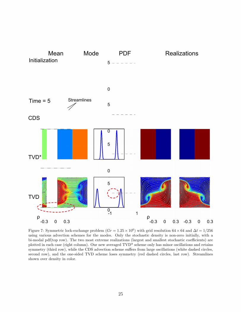
The result of this simulation is shown in Fig. [7] for the three advection schemes. Whilethe CDS scheme maintains symmetry of the mean, modes, pdf, and realizations, some clearnumerical oscillations are present, particularly evident in the realizations. While there areno oscillations in the TVD scheme, it clearly loses symmetry in the mean, modes, pdf, andrealizations, as can be seen (with aid of the dashed guide lines) in Fig. [7]. The TVD*scheme only develops minor oscillations, which can be barely detected when examining therealizations, and completely retains symmetry. Thus, the new TVD* scheme is the preferredscheme among the three.
Initially, we can represent all density realizations exactly with one mode. However, asdifferent densities evolve at different rates, one mode becomes insufficient to represent the
24
Initialization
Time = 5
CDS
TVD*
TVD
-0.3 0 0.3 -0.3 0 0.3 -0.3 0 0.3
-1 10
5
0
5
0
5
0
5
Mean Mode PDF Realizations
ρ ρ
Streamlines
Figure 7: Symmetric lock-exchange problem (Gr = 1.25× 10⁶) with grid resolution 64× 64 and ∆t = 1/256using various advection schemes for the modes. Only the stochastic density is non-zero initially, with abi-modal pdf(top row). The two most extreme realizations (largest and smallest stochastic coefficients) areplotted in each case (right column). Our new averaged TVD* scheme only has minor oscillations and retainssymmetry (third row), while the CDS advection scheme suffers from large oscillations (white dashed circles,second row), and the one-sided TVD scheme loses symmetry (red dashed circles, last row). Streamlinesshown over density in color.
25
uncertainty. Hence, spurious gradients can appear in the reconstructed realizations. Wepurposely chose to use only one mode in this benchmark to also illustrate that if the numberof modes is fixed, errors occur. In general, we do not keep the number of modes fixed [51].
In summary, we found that the TVD* scheme performs adequately and that our DOimplementation can reproduce vastly different realizations of a given problem.
6.3. Numerical Convergence Analysis
The purpose of this benchmark is mainly to show that the implemented scheme is converg-ing. Here we use the classical lid-driven cavity flow, and examine the numerical convergenceunder spatial and temporal refinement of each component separately. This benchmark doesnot have a variable density, and so we report the Reynolds number instead of the Grashoffnumber. We also completed convergence tests with density, with results analogous to thosepresented below.
6.3.1. Numerical Convergence Analysis: Setup
Figure 8: The lid-driven cavity flow is a classical benchmark used to verify convergence of numerical imple-mentations. Uncertainty for this case will be introduced through the initial conditions.
General setup: We present results for a Reynolds number of Re = 500, although otherReynolds number cases (Re ∈ [100, 1000]) were also studied, giving similar results. The flowis driven by a deterministic boundary condition at the top of the enclosed box Fig. [8], withno-slip velocity boundary conditions, and uncertain initial conditions. The finest resolutionuses ∆x = ∆y = 1/512, and ∆t = 1/4096, which is sufficient at this Reynolds number
[12, 11], and the order of convergence is approximated as O ≈ log(‖φ2Nt−φ4Nt‖2‖φ2Nt−φNt‖2
)/ log(2).
We examine the difference between the fine and coarse space resolutions by interpolating(using splines) the fine solution onto the coarse resolution grid, and taking the L2 norm overthe interior of the domain, DI ∈ [0.25, 0.75] × [0.25, 0.75], to avoid the boundary conditionsingularities at the top two corners.
Mean initialization: For a challenging case, the mean velocity and pressure are initiallyzero, everywhere.
Mode initialization: The velocity modes are initialized by specifying the stream function
function δ(x) takes the value 1 if x = 0 and 0 otherwise. The velocity modes are thenspecified as
ui = − ∂
∂yψ(M,N)i , vi =
∂
∂xψ(M,N)i ,
where (M,N) = (1, 1), (1, 2), (1, 3). The initial pressure for the modes is specified as zeroeverywhere.
Stochastic coefficient initialization: The pdf is created using 5,000 samples of zero meanGaussian distributions with variances Var(Yr5000,i) = e(1−Mi−Ni). The number of samples isnot critical in this case, since the samples are the same from one run to the next. That is, weonly test spatial and temporal convergence, not stochastic convergence. Since this is, again,a numerical test, the Yi samples are purposely created using a procedure as in §6.2,
Y ∗r,i =
[Yr5000,i−Yr5000,i
].
To ensure that the final generated samples have numerical variances exactly as specified, wecorrect the samples using the numerically calculated variance
Yr,i = Y ∗r,i
√Var(Yr5000,i)√Varq(Yr,i)
,
where Varq(ar,i) = 1q−1
∑qr=1 ar,i is the calculated sample variance. The initialization for this
problem can be seen in the first row of Fig. [9].
6.3.2. Numerical Convergence Analysis: Results and Discussion
Three time snapshots of the reference solution are shown in Fig. [9]. While the marginalseems to remain approximately Gaussian, the sample-scatter diagram clearly shows the verynon-Gaussian behavior for this benchmark. Also, we confirm from Fig. [10] that the variancesof the modes are decreasing, which is expected since this problem has a deterministic steady-state solution. Thus, the stochastic solution is behaving as expected.
Next, examining the convergence, we see that the numerical error for all components de-crease with temporal and spatial refinement. The convergence is near optimal at large gridsizes for all variables. These results with the velocity components separated are tabulatedin Table [1] and Table [2], which also shows that the stochastic coefficients are convergingoptimally. Even though a fourth-order RK method is used to advance the stochastic coef-ficients, the total-DO convergence is first order (based on choices made in §3.5). Thus, weobserve near-optimal convergence for all variables, which suggests that the implementationis correct.
6.4. Stochastic Convergence
The purpose of the fourth benchmark is to further assess numerical performance, demon-strate that a significant number of modes can be used, and study the effect of the stochasticdiscretization. Specifically, we quantify the effects on accuracy of the number of stochastic
27
−2 2−1
1
InitializationMean Mode 1 Mode2 Mode 3
Mar
gina
l PD
Fs
P
-0.5
0
0.5
−2 2−1
1
Time = 2.5
Mar
gina
l PD
Fs
P
-0.5
0
0.5
Y1
Y2
Y1
Y2
−2 2−1
1Sample Scatter
Time = 5
Mar
gina
l PD
Fs
P
-0.5
0
0.5
Y1
Y2
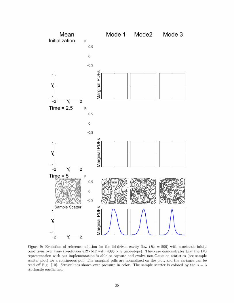
Figure 9: Evolution of reference solution for the lid-driven cavity flow (Re = 500) with stochastic initialconditions over time (resolution 512×512 with 4096 × 5 time-steps). This case demonstrates that the DOrepresentation with our implementation is able to capture and evolve non-Gaussian statistics (see samplescatter plot) for a continuous pdf. The marginal pdfs are normalized on the plot, and the variance can beread off Fig. [10]. Streamlines shown over pressure in color. The sample scatter is colored by the s = 3stochastic coefficient.
28
0 2.5 5Time
Mean
1
2
3
100
10-1
10-2
10-3
Ene
rgy
Figure 10: Evolution of the stochastic energy (Var(Yi)) for the lid-driven cavity reference solution. Thetick-marks on the time-axis corresponds to the time snapshots in Fig. [9].
Figure 11: The control volume size is held fixed at ∆x = 1/512 for the time convergence (left), and the timestep size is held fixed at ∆t = 1/4096 for the spatial convergence (right). The error (‖φ2N −φN‖2) decreaseswith both temporal- and spatial-refinement for each component, and convergence is near-optimal (order 1in time and 2 in space).
Figure 12: Laminar vortex shedding over a square cylinder in a channel. Here uncertainty originates from theinitial conditions and uncertain vortex shedding: depending on the perturbation, the first vortex could eitherbe shed above or below the cylinder. Within a stochastic framework, however, if uncertainties are initiallysymmetric, the mean and modes should remain symmetric, and this is evaluated with our DO numerics.
29
. Nt Mean Mode 1 Mode 2 Mode 3‖e‖2 O ‖e‖2 O ‖e‖2 O ‖e‖2 O
Table 1: Temporal convergence of lid-driven cavity flow. Tabulated is the error (e = ‖φ2Nt−φNt
‖2) betweenthe solutions using ∆t = 1/(2Nt) and using ∆t = 1/Nt, and the approximate order of convergence O. Thegrid size is fixed at ∆x = 1/512.
samples and of the time-order of integration. To do so, we extend the classic shedding of vor-tices by a uniform flow as it encounters a symmetric obstacle to stochastic DO computations.Since this problem is symmetric, the stochastic solution can only lose symmetry if numericalor external perturbations initiate the non-symmetric laminar shedding of vortices. However,if perturbations are symmetric, there should be no preferential direction for vortex shedding.Thus, a carefully initialized simulation should be able to capture symmetric directions: thisprovides an excellent test to assess numerical performance.
6.4.1. Stochastic Convergence: Setup
The benchmark is an open flow in a frictionless pipe with a square cylindrical obstacle(Fig. [12]), which is a classic test for deterministic flow solvers.
General setup: We present results for a Reynolds number of Re = 100, although othercases were also studied. The flow is driven by a deterministic uniform inlet boundary con-dition (left of domain), with slip velocity boundary conditions at the top and bottom, openboundary conditions at the outlet, and symmetric uncertain initial conditions. All simula-tions use a resolution of 336 × 63 in space, and 63 × 40 in time. We choose to integrateuntil t = 40 because this allows the statistics to reach steady values. At t = 40 the meanvelocity has traveled through the domain 2.5 times.
Mean initialization: The mean velocity and pressure are initially zero, everywhere.Mode initialization: The exact shape of the initial stochastic perturbations are not im-
portant since they are advected out of the domain. However, to maintain symmetry, per-turbations have to be symmetric. We initialize the velocity modes by specifying the streamfunction
Table 2: Spatial convergence of lid-driven cavity flow. Tabulated is the error (e = ‖φ2Nx − φNx‖2) betweenthe refined (2Nx×2Nx) and present (Nx×Nx) grid, and the approximate order of convergence O. The timestep is fixed at its smallest value ∆t = 1/4096.
where CM,N is the normalization constant (as in §6.3), and a = 16, b = 3 are the width andheight of the domain respectively. The velocity modes are then specified as
and BM is a smoothing function created numerically from the domain mask. BM is createdfrom the mask by iteratively averaging each control volume by its own value and its fourneighbors for 2
∆yiterations. That is, at iteration k
BkM(i, j) =
1
5
(Bk−1M (i, j) +Bk−1
M (i− 1, j) +Bk−1M (i, j − 1)
+Bk−1M (i+ 1, j) +Bk−1
M (i, j + 1)).
The initial pressure for the modes is specified as zero everywhere.Stochastic coefficient initialization: To ensure initial symmetry, the samples for the
stochastic coefficients are created using the same procedure as in §6.3, using the variancesV ar(Yr,i) = e(2−Mi−Ni) (note the difference of +1 in the exponential from §6.3). The referencesolution uses 105 samples for the stochastic coefficients, and a 4th order RK time integrationscheme (§3.5).
31
1
-1
0M
ean
Mod
e 1
Mod
e 2
Mod
e 3
Mod
e 4
Mod
e 5
Marginal PDFs
0
Ene
rgy
Mean Mode 1
Mode 10
Time 4010
-4
10-2
100
102
Figure 13: Mean field and first 5 modes with marginal pdfs at final non-dimensional time T=40 for Re=100,and the evolution of the mean, 〈u,u〉D and stochastic energy, Var(Yi), for the reference solution (resolution63×336 with 63 × 40 time-steps). Streamlines shown over pressure in color. Our scheme and implementationretains (anti)-symmetry for the most important first four modes.
32
Figure 14: As in Fig. [13], but showing two realizations where the vortex is shed in opposite directions. Thecolorbar for the pressure is as on Fig. [13].
0 40−4
−2
0
2
1e51e41e31e2
O(1)O(2)O(4)
Order
# of Samples
Mode12
3
5
10
12
3
5
10
Time
Ene
rgy
Ene
rgy
Mode
10
10
10
10
−4
−2
0
2
10
10
10
10
Figure 15: Energy of the stochastic coefficients, Var(Yi), over time for: (top) different number of samples(O(4) time integration); and (bottom), different time integration schemes (10,000 samples). Trends are wellcaptured in all cases, but there are noticeable errors for less energetic modes after long integration times whena small number of samples and a low order time discretization scheme is used. A relatively small numberof samples (10,000) can be used for this benchmark since nearly identical results compared to 100,000 werefound for the most energetic four modes.
33
Mode 2
Samples:Order:
1e2O(4)
1e3O(4)
1e4O(4)
1e4O(2)
1e4O(1)
1e5O(4)
Mode 1
Mode 4
Mode 3
Mode 5
Figure 16: Marginal probability density functions of first five modes for the flow over a square cylinderbenchmark at final time (columns 1-3, increasing sample sizes; columns 4-5, decreasing order in time; column6, reference). With 10,000 samples for the stochastic coefficients, the continuous marginal pdfs are well-represented, although the bimodal peaks lose some symmetry. The marginals have similar shapes for allsample sizes, but the best representations have larger sizes. Overall, the order of the time-integrationscheme has less effect than the sample size (the overall order in time is one).
34
6.4.2. Stochastic Convergence: Results and Discussion
For the reference solution, we find that excellent symmetry is maintained for the first fourstochastic modes (Fig. [13]). From the realizations (Fig. [14]), the scheme clearly capturesboth shedding directions. We find that for fewer samples and lower time integration accuracy,the symmetry is not as well maintained (not shown). However, for a sufficient number ofsamples, symmetry is maintained for all Reynolds numbers we tested. From Fig. [13], wesee that variances seem to reach a steady value after an initial transient period. The smallervariances take longer to reach a steady value; the highest modes still evolve after the finaltime step.
For our sequential implementation, the reference DO simulation (Fig. [13]) was computedin about 7.5 hours on a 2.4Ghz computer. Each time-step required the inversion of 11pressure equations, as opposed to the 111 required for the scheme without the stochasticpseudo pressure. This roughly translates to a 1000 % increase in efficiency, or about 3 dayssaving in terms of computational time for this computer. Since then, we have used as manyas s = 25 modes for data assimilation applications [56, 57].
Sample sizes: Examining the evolution of the stochastic coefficients for different samplesizes (top of Fig. [15]), we see that the differences are larger for higher modes. For themost energetic first four coefficients, the results agree well with the reference solution whenusing > 1, 000 samples. After the 5th coefficient, the differences become larger, and inthe 10th coefficient, the differences begin sooner and have larger relative magnitudes. Notethat the logarithmic scale magnifies smaller errors, and the differences for the 10th are fullyinsignificant when compared to the variance of the first mode. Thus, with a relatively smallnumber of samples, it is possible to capture the stochastic coefficient’s variances accurately.Also, it appears as though the solution converges when the number of samples increases,which increases our confidence in this approach.
Not only are the evolution of the variances well-represented by a smaller number ofsamples, the shape of the marginals are also well-reproduced (Fig. [16]). We observe that themarginals are well-reproduced using > 1, 000 samples, and for all time integration schemes(Fig. [16]). The magnitudes of the bimodal peaks in the first mode are more symmetricwith increased sample sizes, which suggests using upwards of 10,000 samples is, perhaps,advised. In fact, using such a number of samples does not affect the overall cost of thesolution scheme. That the marginals are well-represented using smaller sizes is encouraging,since it suggests that a small number of samples (that won’t negatively impact the efficiencyof the scheme) could be used for problems with large s: this would not substantially affectaccuracy.
Order in time: We are here only varying the order of the ODE solver used to evolve thestochastic coefficients: the overall order of the DO scheme is kept fixed at first order (see§3.4). Examining results (bottom of Fig. [15]), we see that the second and fourth orderODE solver agree well for all coefficients. A second order solver thus seems sufficient.
In summary, we simulated a stochastic version of the classical flow over a square cylinderbenchmark. We found that our DO solver maintains excellent symmetry, and the use ofpseudo-pressures reduces the cost by 1000% when using 10 stochastic modes. We also foundthat the statistics is converging with the number of samples and that accuracy benefitsfrom using a second-order solver for the coefficients, even though the overall DO scheme is
35
limited to first order. Finally, smaller sample sizes for the coefficients still produced accuratetime-evolving statistic and marginal pdfs, which is encouraging.
7. Conclusions and Future Research
We have derived efficient computational schemes for the DO methodology applied tounsteady stochastic Navier-Stokes and Boussinesq equations, and illustrated and studiedthe numerical aspects of these schemes. For the discretizations in time, we developed semi-implicit projection methods for the mean and the modes, and we employed time-marchingschemes of first to fourth order for the stochastic coefficients. For the discretizations of thephysical space, we employ conservative second-order finite-volumes, with a special treatmentfor the advection terms based on a TVD scheme with monotonized central symmetric fluxlimiter. Several alternate discretizations in time and space were outlined and illustrated bycomparisons. We also addressed several numerical issues specific to the DO method for fluidand ocean flows. In particular we have shown: how to define pseudo-stochastic pressuresto reduce the number of matrix inversions for the pressure from O(s2) to O(s); how totreat advection by the stochastic modes using symmetric approximate TVD schemes; howto deal with singular subspace covariances by generalized inversion; and how to maintainorthonormal modes at the numerical level and so account for truncation and round-off errorsduring time integration. Finally, we evaluated our schemes using a varied set of stochasticflows, hence illustrating robustness but also providing benchmarks for future schemes andimplementations.
Using an asymmetric Dirac-stochastic lock-exchange benchmark, we found excellent agree-ment among multiple realizations from a deterministic code and the realizations generatedfrom a single stochastic simulation. This validated our numerical implementation, and con-firmed that the pseudo-stochastic pressure approach works in practice. Using a symmetricversion of the lock-exchange benchmark, we showed that the symmetric TVD advectionscheme (TVD*) works well, while the CDS scheme suffers from numerical oscillations, andthe non-symmetric TVD scheme loses symmetry.
Using a lid-driven cavity flow with uncertain initial conditions, we showed that each com-ponent converged near-optimally under both time and space refinement. Additionally, weshowed that even when a higher-order time integrator is used for the stochastic coefficients,their accuracy is still limited to approximately first order, as discussed in §3.4. This bench-mark also demonstrated an expected decay in the variance of the stochastic coefficients,which were shown to be very non-Gaussian.
Finally, using a stochastic flow past a square cylinder in a confined channel, we showedthat the stochastic coefficients converged with increased samples sizes and orders of time in-tegration. We found that using > 10, 000 samples and a second order time-integrator yieldedadequate performance. This benchmark also demonstrated that our discretized DO method-ology successfully captures both vortex shedding directions, resulting in a fully symmetricmean field. Also, we noted that using our newly defined pseudo-stochastic pressure, we were1000% more efficient computationally when using 10 modes.
Possible future studies include the efficient extension of our present framework to flowswith uncertain parameters in the governing equations and with stochastic forcing at theboundary and in the interior. Also, our results suggest that simulations with long time
36
integration will benefit from more accurate time-integration scheme. Then, while our pro-posed symmetric TVD-based advection and orthonormalization schemes for the stochasticmodes were shown to perform adequately, more optimal treatments are possible. Alternativemeans of discretizing the stochastic coefficients are worth exploring for applications whererare events are important. Finally, specific multi-resolution DO schemes can be derived formultiscale stochastic fluid and ocean flows. Unstructured grids as well as nested approaches[8, 18] will then be useful. The utilization of the present schemes as well as these future ad-vances will allow the prediction of uncertainty in realistic simulations of multi-physics fluidsystems, over a wide range of applications, from micro-nano fluid engineering to multiscaleocean and climate studies.
8. Acknowledgements
We are very thankful to the MSEAS group members, in particular Mr. Sondergaard and
Mr. Lolla for helpful discussions. We thank Dr. Shirokoff for the many discussions about Projection
methods. We are grateful to the Office of Naval Research for support under grants N00014-08-1-1097
(ONR6.1), N00014-09-1-0676 (QPE) and N00014-09-1-0676 (Science of Autonomy – A-MISSION)
to the Massachusetts Institute of Technology (MIT). MPU and PFJL also thank the Natural Sci-
ences and Engineering Research Council (NSERC) of Canada for the Postgraduate Scholarship
partially supporting the graduate studies and research of MPU at MIT.
Appendix A. DO Navier-Stokes Equations
In this Appendix we present the stochastic DO equations for Boussinesq dynamics, andbriefly summarize the required steps (from [50, 49, 52]) to obtain these equations.
Starting with a generalized Karhunen-Loeve expansion [32, 49], one decomposes the so-lution of eqns. (1)-(3) into a Dynamically Orthogonal (DO) field expansion [50, 49, 51] forthe velocity, density and pressure2 fields
Φ(x, t;ω) = Φ(x, t) +s∑i=1
Yi(t;ω)Φi(x, t),
Φ ≡ Φ + YiΦi,
(A.1)
p(x, t;ω) = p(x, t) +s∑i=1
Yi(t, ω)pi(x, t) +s∑i=1
s∑j=1
Yi(t;ω)Yj(t;ω)pij(x, t),
p ≡ p+ Yipi + YiYjpij,
(A.2)
where Φ = [Φ1,Φ2, . . .]T = [u, ρ]T is the vector of prognostic state variables. The scalars = s(t) defines the time-dependent dimension of the stochastic subspace, i.e. s is a discretenumber of stochastic terms retained from a complete expansion. The field functions Φi(x, t)are the s orthonormal deterministic modes and the Yi(t;ω) are their s zero-mean stochastic
2For convenience, we changed the sign of pij from the original definition in the Sapsis and Lermusiaux[50]
37
coefficients, in general non-Gaussian. In our notation, we use the Einstein summation ex-clusively for summations related to the stochastic expansion. The decomposition of pressureinto a mean, linear modal and quadratic modal component follows from the Pressure PoissonEquations (see §3.2 or Sapsis and Lermusiaux [50]). Since both the modes and stochasticcoefficients are functions of time, a redundancy arises, which is resolved by the DO condition,⟨
Φi,∂Φj
∂t
⟩D
= 0, ∀i, j ∈ [1, 2, . . . , s], (A.3)
where the inner product is defined as 〈a,b〉D =∫D∑
i(aibi) dD for arbitrary vectors of
spatial functions a = [a1, a2, . . .]T and b = [b1, b2, . . .]T .Using the DO condition, an exact set of equations can be obtained that governs the
evolution of the mean, modes, and stochastic coefficients of the generalized Karhunen-Loeveexpansion. The only approximation arises from the truncation of the DO expansion to s(t)terms. First substitute (A.1) into eqns. (1)-(3) to obtain (using a Langevin notation):
∂u
∂t+dYidt
ui + Yi∂ui∂t
= Lu (u + Yiui, ρ+ Yiρi, p,x, t;ω) ,
∂ρ
∂t+dYidtρi + Yi
∂ρi∂t
= Lρ (ρ+ Yiρi, u + Yiui,x, t;ω) ,
(A.4)
and DO decomposed versions of (2)-(3). It is from these equations, within which the DOdecomposition was inserted, that the equations for the mean, modes and their coefficients areobtained, using the expectation operator, the spatial inner product, and eqns. (A.2)-(A.3).
Mean. To obtain a rate of change for the mean fields, the idea is to eliminate the randomcomponents in the left-hand-sides of eqns. (A.4). Hence, taking the expectation of eqns. (A.4)it can be found that the evolution of the mean fields are governed by
∇ · u = 0, x ∈ D,∂u
∂t− 1√
Gr∇2u = −∇ · (uu)−∇p+ ρeg
−CYiYj (∇pij +∇ · (ujui)) , x ∈ D,∂ρ
∂t− 1
Sc√Gr∇2ρ = −∇ · (uρ)−CYiYj∇ · (ujρi), x ∈ D,
(A.5)
with the initial and boundary conditions given by
u (x, 0) = u0, x ∈ D,ρ (x, 0) = ρ0, x ∈ D,
(A.6)
u = gD, x ∈ ∂DD,∂u
∂n= gN , x ∈ ∂DN ,
ρ = gDρ , x ∈ ∂DDρ ,∂ρ
∂n= gNρ , x ∈ ∂DNρ ,
(A.7)
38
where CYiYj = Eω [YiYj] is an element of the covariance matrix in the stochastic/errorsubspace. Deterministic initial and boundary conditions ( • quantities) are assigned tothe mean. Note that in general the vector ∇ · (ujui) differs from ∇ · (uiuj) (recall that
∇ · (ujui)q =∂ujruiq∂xr
6= ∂uirujq∂xr
; e.g.,∂vjui∂y6= ∂viuj
∂y).
Modes. The evolution of the modes is also obtained from eqns. (A.4). To do so, theidea is to eliminate the random coefficients in front of the time derivatives of the modes.The essential steps are to multiply these equations with a stochastic coefficient Yj, applythe expectation operator, and substitute an expression for Eω
[∂Yi∂tYj], which is obtained by
projecting the equation unto Φk and imposing the DO condition. From this the followinggoverning evolution equations for the modes can be found:
∇ · ui = 0, x ∈ D,∂ui∂t
= Qui − 〈Qi,Φj〉D uj , x ∈ D,
∂ρi∂t
= Qρi − 〈Qi,Φj〉D ρj , x ∈ D,
(A.8)
where
Qi = [Qui ,Q
ρi ]T =
[C−1YiYj
Eω [Lu Yj] , C−1YiYj
Eω [Lρ Yj]]T,
Qui =
1√Gr∇2ui −∇ · (uiu)−∇ · (uui)−∇pi + ρie
g
−C−1YiYj
MYjYmYn (∇pmn +∇ · (unum) ) ,
Qρi =
1
Sc√Gr∇2ρi −∇ · (uiρ)−∇ · (uρi)
−C−1YiYj
MYjYmYn (∇ · (unρm) ) ,
and MYjYmYn = Eω [YjYmYn] is a third moment. The right-hand-sides in eqns. (A.8) corre-spond the total rate of change of the subspace (without a DO condition) minus the projectionof this rate of change on the subspace itself (which is subtracted to ensure the DO condition).We note that in general ∇ · (uui) 6= ∇ · (uiu) since ∂vui
∂y6= ∂viu
∂yfor example.
The initial and boundary conditions for the modes are obtained from those of the fullstochastic fields, eqns. (2) and (3), but reduced to their dominant initial error subspace ofsize s0,
ui (x, 0) = ui,0 (x) , x ∈ D,ρi (x, 0) = ρi,0 (x) , x ∈ D,
(A.9)
39
and
ui = gi,D, x ∈ ∂DD,∂ui∂n
= gi,N , x ∈ ∂DN ,
ρi = gi,Dρ , x ∈ ∂DDρ ,∂ρi∂n
= gi,Nρ , x ∈ ∂DNρ .
(A.10)
Coefficients. Finally, to obtain the evolution of the stochastic coefficients from eqns. (A.4),the idea is to eliminate the modes in the term containing the time derivatives of the ran-dom coefficients. To do so, project the evolution eqns. (A.4) onto each mode i, apply theDO conditions, and essentially impose that each coefficient is of zero mean. The resultinggoverning stochastic ODEs are
dYidt
= 〈L − Eω [L] ,Φi〉D ,
= 〈Fm,Φi〉D Ym − 〈∇pmn +∇ · (unum),ui〉D (YmYn −CYmYn)
− 〈∇ · (unρm), ρi〉D (YmYn −CYmYn) ,
(A.11)
where L = [Lu,Lρ]T and Fm = [Fum,F
ρm]T with
Fum =
1√Gr∇2um −∇ · (umu)−∇ · (uum)−∇pm + ρmeg,
Fρm =
1
Sc√Gr∇2ρm −∇ · (umρ)−∇ · (uρm),
The initial conditions for the coefficients are obtained from those of the full stochasticfields, eqn. (2), by projection onto each initial mode i, Φi,0, and removal of the mean. Thisleads to:
In this Appendix we stated the DO equations for the mean, modes, and stochastic coef-ficients of the stochastic Boussinesq equations.
Appendix B. Numerical orthonomalization procedure
In this Appendix, we present our newly developed, numerically efficient, orthonormaliza-tion procedure based on the discussion in §5.2.
Consider the pictorial analogy showing different strategies when orthonormalizing the ba-sis (Fig. [B.17]). In case (a), the argument is that the coefficients were evolved correctly, andall the error lies in the basis evolution. This is not true because we evolve the coefficients bytaking an inner product of the equations using the bases at the old time-step. In case (b), theargument is that the energy and ‘direction’ of the realizations were correctly evolved. When
40
(Y,Y)1 2
(Y',Y')1 2
(Y,Y)1 2
(Y',Y')1 2
(Y,Y)1 2
(Y',Y')1 2
a) Orthonormalizebasis withoutmodifying coefficients
c) Orthonormalizebasis withoutmodifyingrealizations
b) Orthonormalizebasis and retainrealizationenergy and 'direction'
Y'=Y i i Cov(Y')=Cov(Y)i i Y'Φ'=YΦ i i i i
Φ1
Φ2
Φ'1
Φ'2
Φ1
Φ2
Φ'1
Φ'2
Φ1
Φ2
Φ'1
Φ'2
Figure B.17: There are different ways to treat the stochastic coefficients when orthonormalizing the modes.In this pictorial analogy, the standard 2D cartesian bases and coordinates represent the modes and stochasticcoefficients, respectively.
correcting the bases, the direction and energy are maintained, but the actual realization ismodified. In case (c), the argument is that the realizations were evolved correctly. However,it is unlikely that the errors in the modes and coefficients cancel during the time evolution.Also, while not evident from the pictorial analogy, the energy of the coefficients change incase (c). This is because the length of the basis changes when orthonormalized, and thislength change is then accounted for in the coefficients in order to maintain the coordinateof the realization. The case (b) strategy is a compromise between cases (a) and (c), and itresults in the lowest error for the lock-exchange cases in §6.1. The errors were the largestfor case (a), and the errors for case (c) were marginally larger compared to case (b).
To be clear, case (b) is shown to perform best for the specific cases in §6.1, and theseresults are not proven to be universally applicable. Also, we made no attempt to provide anexhaustive list of all the orthonormalization strategies. For example, arguing that the coef-ficients still live in the bases of the old timestep, one can consider projecting the coefficientsfrom this old basis onto the new basis before orthonormalization. Therefore, the issue of theoptimal orthonormalization strategy is left open to future research. Nonetheless, we believeour current approach is sufficient for most applications since no strategy will influence thescheme’s overall order of accuracy. Any improved strategy will only reduce the size of theerror, which will be of order ∆t smaller than the truncation error. Therefore, any accuracyissues due to orthonormalization can be resolved by reducing the size of the timestep whenusing the current scheme. Our orthonormalization procedure for case (b) is described next.
For case (b), we want the new orthonormalized basis to: approximately recover the spe-cific realizations before the orthonormalization; and exactly maintain the stochastic energy.Mathematically we, ideally, want both:
Φh,i(Yr,i)T ≈ ΦO
h,i(YOr,i)
T , (B.1)
Tr(Ck?Yr,iYr,j
) = Tr(Ck?,OYr,iYr,j
), (B.2)
where the orthonormalized basis is defined such that⟨ΦOh,i,Φ
Oh,j
⟩D = δij, and the trace
operator Tr simply sums the diagonal entries of a matrix. In order to preserve the second
41
property, we first rotate the stochastic system such that the covariance matrix is diagonal:
CkYiYj
= E[Yr,iYr,j] = VDCDDCVTDC , (B.3)
Y DCr,i = Yr,iVDC , (B.4)
ΦDCh,i = Φh,iVDC , (B.5)
which gives the decorrelated (or DC) stochastic coefficients. By starting with a decorrelatedsystem, we have a unique and convenient reference frame which we can use to enforce theTr(Ck?
YiYj) property.
Next we perform the orthonomalization as follows
Mij =⟨ΦDCh,i ,Φ
DCh,j
⟩D = VMDMVT
M , (B.6)
Y OCr,i = Y DC
r,i VM
√DM , (B.7)
ΦOCh,i = ΦDC
h,i VM
√D−1M . (B.8)
The above could be accomplished by directly calculating the Singular Value Decompositionof the ΦDC
h,i matrix, but the above procedure has the advantage of enabling the user to specifyany desired (possibly non-linear) inner product. In either case, the two approaches are similarin efficiency and give the same results. To verify that (B.1) is satisfied, we substitute theabove expression in (B.1)
ΦDCh,i (Y DC
r,i )T = ΦOCh,i (Y OC
r,i )T ,
= ΦDCh,i VM
√D−1M
(Y DCr,i VM
√DM
)T,
= ΦDCh,i VM
√D−1M
√DMVT
M(Y DCr,i )T ,
= ΦDCh,i (Y DC
r,i )T ,
since the eigen-vectors are orthonormal VMVTM = I. Therefore the first property, (B.1), is
exactly satisfied at this stage. Stopping here would give the case (c) strategy.Finally, we decorrelate the samples again, while ensuring that the stochastic energy is
preserved:
Ck,OCYiYj
= E[Y OCr,i Y
OCr,j ] = VODOVT
O, (B.9)
Y Or,i = Y OC
r,i VO
√Tr(DDC)
Tr(DO), (B.10)
ΦOh,i = ΦOC
h,i VO. (B.11)
Note that Tr(DO) = Tr(DDCDM), but that DO 6= DDCDM . This ensures that (B.2) ismaintained, but now we can only approximately satisfy (B.1). The over-all correction is
42
then as follows:
Y Or,i = Yr,iVDCVM
√DMVO
√Tr(DDC)
Tr(DO), (B.12)
ΦOh,i = Φh,iVDCVM
√D−1M VO. (B.13)
This procedure is robust even if Ck,OCYY is singular, however it does require a non-singular
Mij which will normally be the case if modes are properly initialized. Also, the number offloating point operations is dominated by the calculation of Mij if the number of spatial pointsexceeds the number of realizations. Nonetheless, the overall cost of the orthonormalizationis inexpensive compared to the inversion of the pressure Poisson equations.
References
[1] Bennett AF (1992) Inverse Methods in Physical Oceanography., 1st edn. Cambridge University Press, New York
[2] Cameron RH, Martin WT (1947) The orthogonal development of nonlinear functionals in series of Fourier-Hermite func-tionals. Ann of Math 48:385–392
[3] Carpenter MH, Kennedy C (1994) Fourth-order 2N-storage Runge-Kutta schemes. NASA Report TM 109112, NASALangley Research Center, Hampton, VA
[4] Chapra SC, Canale RP (2006) Numerical Methods for Engineers, 5th edn. McGraw-Hill Higher Education, Boston, MA
[5] Chen D, Liu J (2000) Mixture Kalman filters. J Roy Statist Soc Ser A 62:493–508
[6] Cushman-Roisin B, Beckers JM (2010) Introduction to geophysical fluid dynamics: Physical and Numerical Aspects.Academic Press.
[7] Deb MK, Babuska I, Oden J (2001) Solution of stochastic partial differential equations using Galerkin finite elementtechniques. Comput Methods Appl Mech Eng 190:6359–6372
[8] Deleersnijder E, Lermusiaux PFJ (2008) Multi-scale modeling: nested grid and unstructured grid approaches. OceanDynamics 58:335–336
[9] Doucet A, de Freitas N, Gordon N (2001) Sequential Monte-Carlo Methods in Practice. Springer-Verlag
[10] Eldred MS, Webster CG, Constantine P (2008) Evaluation of Non-Intrusive Approaches for Wiener-Askey GeneralizedPolynomial Chaos. In: Proceedings of the 49th AIAA/ASME/ASCE/AHS/ASC Structures, Structural Dynamics, andMaterials Conference (10th AIAA Non-Deterministic Approaches Conference), paper AIAA-2008-1892, Schaumburg, IL
[11] Erturk E (2009) Discussions on driven cavity flow. Int J Numer Meth Fluids 60:275–294
[12] Erturk E, Corke TC, Gokcol C (2005) Numerical Solutions of 2-D Steady Incompressible Driven Cavity Flow at HighReynolds Numbers. Int J Numer Meth Fluids 48:747–774
[13] Ferziger JH, Peric M (2002) Computational Methods for Fluid Dynamics, 3rd edn. Springer, New York, NY
[14] Foo J, Karniadakis GE (2010) Multi-element probabilistic collocation method in high dimensions. J Comput Phys 229:1536–1557
[15] Frochte J, Heinrichs W (2009) A splitting technique of higher order for the Navier-Stokes equations. J Comput Appl Math228:373–390
[16] Ghanem R, Spanos P (1991) Stochastic Finite Elements: A Spectral Approach. Springer-Verlag
[17] Guermond J, Minev P, Shen J (2006) An overview of projection methods for incompressible flows. Comput Methods ApplMech Engrg 195:6011–6045
[18] Haley PJ Jr, Lermusiaux PFJ (2010) Multiscale two-way embedding schemes for free-surface primitive-equations in theMultidisciplinary Simulation, Estimation and Assimilation System (MSEAS). Ocean Dynamics 60:1497–1537
[19] Hartel C, Meiburg E, Necker F (2000) Analysis and direct numerical simulation of the flow at a gravity-current head. Part1. Flow topology and front speed for slip and no-slip boundaries. J Fluid Mech 418:189–212
[20] Higham DJ (2001) An Algorithmic Introduction to Numerical Simulation of Stochastic Differential Equations. SIAMReview 43(3):525–546
[21] Hosder S, Walters R, Perez R (2006) A nonintrusive polynomial chaos method for uncertainty propagation in CFDsimulations. In: AIAA Aerosp. Sci. Meet. Exhib, 44th, AIAA-2006-0891, Reno, Nevada
43
[22] Jakeman JD, Roberts SG (2008) Stochastic Galerkin and collocation methods for quantifying uncertainty in differentialequations: a review. Aust NZ Ind Appl Math J 50:C815–C830
[23] Karhunen K (1946) Zur spektraltheorie stochastischer prozesse. Ann Acad Sci Fennicae 34:17
[24] Kloeden PE, Platen E (1999) Numerical Solution of Stochastic Differential Equations. Springer-Verlag, Berlin
[25] Le Maıtre O, Reagan M, Najm H, Ghanem R, Knio O (2002) A stochastic projection method for fluid flow II. Randomprocess. J Comput Phys 181:9–44
[26] Le Maıtre O, Najm H, Ghanem R, Knio O (2004) Multi-resolution analysis of Wiener-type uncertainty propagationschemes. J Comput Phys 197:502–531
[27] Le Maıtre OP, Knio OM (2010) Spectral Methods for Uncertainty Quantification, 1st edn. Scientific Computation, Springer,New York
[28] Le Maıtre OP, Knio OM, Najm HN, Ghanem RG (2001) A Stochastic Projection Method for Fluid Flow I. Basic Formu-lation. J Comput Phys 173:481–511
[29] Lermusiaux PFJ (1999) Data assimilation via error subspace statistical estimation. Part II: Middle atlantic bight shelfbreakfront simulations and ESSE validation. Mon Weather Rev 127:1408–1432
[30] Lermusiaux PFJ (2001) Evolving the subspace of the three-dimensional multiscale ocean variability: Massachusetts Bay.J Mar Syst 29:385–422
[31] Lermusiaux PFJ (2002) On the mapping of multivariate geophysical fields: Sensitivities to size, scales, and dynamics. JAtmos Ocean Technol 19(10):1602–1637
[32] Lermusiaux PFJ (2006) Uncertainty estimation and prediction for interdisciplinary ocean dynamics. J Comput Phys217:176–199
[33] Lermusiaux PFJ (2007) Adaptive Modeling, Adaptive Data Assimilation and Adaptive Sampling. Physica D 230:172–196,Special issue on “Mathematical Issues and Challenges in Data Assimilation for Geophysical Systems: InterdisciplinaryPerspectives.” C.K.R.T. Jones and K. Ide, Eds.
[35] Lermusiaux PFJ, Robinson AR (1999) Data assimilation via error subspace statistical estimation. Part I: Theory andschemes. Mon Weather Rev 127:1385–1407
[36] Lermusiaux PFJ, Chiu CS, Gawarkiewicz G, Abbot P, Robinson A, Miller R, Haley P, Leslie W, Majumdar S, Pang A,Lekien F (2006) Quantifying uncertainties in ocean predictions. Oceanography 19:92–105
[37] Leveque RJ (2002) Finite Volume Methods for Hyperbolic Problems. Cambridge University Press
[38] Li R, Ghanem R (1998) Adaptive polynomial chaos expansions applied to statistics of extremes in nonlinear randomvibration. Prob Eng Mech 13:125–136
[39] Loeve M (1977) Probability Theory. Springer-Verlag, Berlin/New York
[43] Mathelin L, Hussaini MY, Zang TA (2005) Stochastic approaches to uncertainty quantification in CFD simulations. NumerAlgor 38(1-3):209–236
[44] McLachlan G, Peel D (2000) Finite mixture models. Wiley series in probability and statistics: Applied probability andstatistics, Wiley
[45] van der Merwe R, Wan E (2003) Gaussian mixture sigma-point particle filters for sequential probabilistic inference indynamic state-space models. In: Proceedings of the International Conference on Acoustics, Speech, and Signal Processing,ICASSP, Hong-Kong
[46] Miller R (2007) Topics in data assimilation: Stochastic processes. Physica D 230(1-2):17 – 26
[47] Najm HN (2009) Uncertainty Quantification and Polynomial Chaos Techniques in Computational Fluid Dynamics. AnnuRev Fluid Mech 41:35–52
[48] Nouy A (2007) A generalized spectral decomposition technique to solve a class of linear stochastic partial differentialequations. Comput Methods Appl Mech Engrg 196:4521–4537
[49] Sapsis TP (2010) Dynamically orthogonal field equations for stochastic fluid flows and particle dynamics. Ph.D.Thesis,Massachusetts Institute of Technology, Dept. of Mech. Eng.
[50] Sapsis TP, Lermusiaux PFJ (2009) Dynamically orthogonal field equations for continuous stochastic dynamical systems.
44
Physica D 238:2347–2360
[51] Sapsis TP, Lermusiaux PFJ (2011) Dynamical criteria for the evolution of the stochastic dimensionality in flows withuncertainty. Physica D Under Review
[52] Sapsis TP, Lermusiaux PFJ, Ueckermann MP (2011) Statistical model of Navier-Stokes equations using dynamical orthog-onality. J Fluid Mech In preparation.
[53] Shirokoff D, Rosales R (2011) An efficient method for the incompressible Navier-Stokes equations on irregular domainswith no-slip boundary conditions, high order up to the boundary. J Comput Phys 230(23):8619 – 8646
[54] Simon F, Guillen P, Sagaut P, Lucor D (2010) A gPC-based approach to uncertain transonic aerodynamics. ComputMethods Appl Mech Engrg 199(17-20):1091 – 1099
[55] Sondergaard T (2011) Data assimilation with gaussian mixture models using the dynamically orthogonal field equations.S.M.Thesis, Massachusetts Institute of Technology, Dept. of Mech. Eng.
[56] Sondergaard T, Lermusiaux PFJ (2011) Data Assimilation with Gaussian Mixture Models using the Dynamically Orthog-onal Field Equations. Part I: Theory and Scheme. Submitted to Mon Weather Rev
[57] Sondergaard T, Lermusiaux PFJ (2011) Data Assimilation with Gaussian Mixture Models using the Dynamically Orthog-onal Field Equations. Part II: Applications. Submitted to Mon Weather Rev
[58] Timmermans L, Minev P, Van De Vosse F (1996) An approximate projection scheme for incompressible flow using spectralelements. Int J Numer Methods Fluids 22:673–688
[59] Ueckermann MP, Lermusiaux PFJL (In Prep. 2011) 2.29 Finite Volume MATLAB Framework Documentation. Reportsin Ocean Science and Engineering 14, Department of Mechanical Engineering, Massachusetts Institute of Technology,Cambridge, Massachusetts
[60] Van Leer B (1977) Towards the ultimate conservative difference scheme. IV. A new approach to numerical convection. JComput Phys 23(3):276 – 299
[61] Wan X, Karniadakis GE (2005) An adaptive multi-element generalized polynomial chaos method for stochastic differentialequations. J Comput Phys 209:617–642
[62] Wan X, Karniadakis GE (2006) Long-term behavior of polynomial chaos in stochastic flow simulations. Comput MethodsAppl Mech Engrg 195:5582–5596
[63] Webster M, Sokolov A (2000) A methodology for quantifying uncertainty in climate projections. Clim Change 46:417–446
[64] Wiener N (1938) The homogeneous chaos. Amer J Math 60:897–936
[65] Wiener N (1958) Nonlinear Problems in Random Theory. MIT Technology Press and John Wiley and Sons
[66] Xiu D (2009) Fast numerical methods for stochastic computations: A review. Commun Comput Phys 5(2-4):242–272
[67] Xiu D (2010) Numerical Methods for Stochastic Computations: A Spectral Method Approach. Princeton University Press
[68] Xiu D, Karniadakis GE (2002) The Wiener-Askey polynomial chaos for stochastic differential equations. SIAM J SciComput 24:619–644
[69] Xiu D, Lucor D, Su CH, Karniadakis GE (2002) Stochastic Modeling of Flow-Structure Interactions Using GeneralizedPolynomial Chaos. J Fluids Eng 124(1):51–60