COMPUTATIONAL STUDY FOR THE NUMERICAL RESOLUTION …

COMPUTATIONAL STUDY FOR THE NUMERICAL

RESOLUTION OF THERMAL AND FLUID DYNAMIC

PROBLEMS.

Studies: MASTER’S DEGREE IN SPACE AND AERONAUTICAL

ENGINEERING

Student: Cesar David Navas Prada

Director: Carlos David Pérez Segarra

Codirector: Asensio Oliva Llena

Thesis Call: QP 2017-2018

Document: Attachments Report

Barcelona, September 2018

Master Final Thesis Attachments Report

Cesar David Navas Prada 2



CONTENTS

List of Figures ................................................................................................................... 5

List of Tables .................................................................................................................... 6

1. INTRODUCTION ....................................................................................................... 7

1.1. Software ............................................................................................................. 7

2. ATTACHMENT I – DEVELOPED ALGORITHMS ...................................................... 9

2.1. Convection-Diffusion Generic Algorithms............................................................ 9

2.1.1. Numerical Schemes .................................................................................... 9

2.1.2. Numerical Solvers ..................................................................................... 15

2.1.3. Diagonal Flow ............................................................................................ 19

2.1.4. Smith-Hutton Problem ............................................................................... 33

2.1.5. 2D Heat Transfer ....................................................................................... 46

2.2. Fractional Step Method Generic Algorithms ...................................................... 61

2.2.1. R(u) Vector ................................................................................................ 61

2.2.2. R(v) Vector ................................................................................................ 63

2.2.3. Poisson Equation....................................................................................... 65

2.2.4. Velocity to Main Nodes .............................................................................. 66

2.2.5. Driven Cavity ............................................................................................. 68

2.2.6. Flow Around Square Cylinder .................................................................... 81

2.3. Burgers Equation .............................................................................................. 98

2.3.1. Main Code ................................................................................................. 98

2.3.2. DNS........................................................................................................... 99

2.3.3. LES ......................................................................................................... 101

3. ATTACHMENT II - GRAPHICAL RESULTS .......................................................... 103

3.1. Convection-Diffusion Equation ........................................................................ 103

3.1.1. Diagonal Flow .......................................................................................... 103

3.1.2. Smith-Hutton Problem ............................................................................. 107

3.2. Fractional Step Method ................................................................................... 114



3.2.1. Driven Cavity ........................................................................................... 114

3.2.2. Flow Around Square Cylinder .................................................................. 116

3.3. Burgers Equation ............................................................................................ 120



LIST OF FIGURES

Figure 1. Diagonal Flow: Iterations and time [200x200], QUICK, line-by-line (rows+) ... 103

Figure 2. Diagonal Flow: Iterations and time [200x200], QUICK, line-by-line (columns+)

..................................................................................................................................... 104

Figure 3. Diagonal Flow: Iterations and time [200x200], QUICK, point-by-point ............ 105

Figure 4. Diagonal Flow: Iterations and time. a) Upwind, b) second-order Upwind, c) QUICK

..................................................................................................................................... 106

Figure 5. Smith-Hutton: ϕ vs X a) [100x50], b) [200x100], c) [300x150] ........................ 107

Figure 6. Smith-Hutton: Iterations and time [300x150], Upwind, line-by-line.................. 108

Figure 7. Smith-Hutton: Iterations and time [300x150], Fromm, line-by-line .................. 109

Figure 8. Smith-Hutton: Iterations and time [300x150], SMART, line-by-line ................. 110

Figure 9. Smith-Hutton: Iterations and time [300x150], Fromm, line-by-line (rows+) ..... 111

Figure 10. Smith-Hutton: Iterations and time [300x150], Fromm, line-by-line (column+) 112

Figure 11. Smith-Hutton: Iterations and time [300x150], Fromm, Point-by-point ........... 113

Figure 12. 2D Heat Transfer: Results for mesh [30x30] at Re = 400 for validation of the

code ............................................................................................................................. 114

Figure 13. 2D Heat Transfer: Results for mesh [30x30] at Re = 1000 for validation of the

code ............................................................................................................................. 115

Figure 14. Square Cylinder: Velocity Ux at Reynolds a) 1, b) 10, c) 50, d) 60, e) 100, f) 200

..................................................................................................................................... 116

Figure 15. Square Cylinder: Velocity Vy at Reynolds a) 1, b) 10, c) 50, d) 60, e) 100, f) 200

..................................................................................................................................... 117

Figure 16. Square Cylinder: Pseudo-pressure field at Reynolds a) 1, b) 10, c) 50, d) 60, e)

100, f) 200 .................................................................................................................... 118

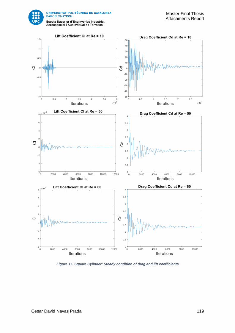
Figure 17. Square Cylinder: Steady condition of drag and lift coefficients ..................... 119

Figure 18. Burgers Equation: Energy spectrum at Re = 1 ............................................. 120

Figure 19. Burgers Equation: Energy spectrum at Re = 100 ......................................... 120

Figure 20. Burgers Equation: Energy spectrum at Re = 300 ......................................... 121



LIST OF TABLES

Table 1. Software licenses used during the study ............................................................. 7



INTRODUCTION

1. INTRODUCTION

This document contains the algorithms self-developed during this study, and the graphical

results that were not relevant enough for the conclusions in the main final report.

It is important to highlight that all cases of study use some generic algorithms. These

generic algorithms were developed as functions in MATLAB. For the convection-diffusion

problems the numerical schemes and numerical solver are generic algorithms, and for FSM

the generics algortihms are the R(u,v) vector and Poisson equation solution code. Specific

functions were required for each case of study regarding the individual equiremnts of the

cases, these MATLAB functions will be presented separered for ech case as well.

Consequently, some extra graphical results are showed and lastly, the document also

includes the software description and the license permits required for this study.

1.1. Software

This study was performed mainly in a computational environment; therefore, the licenses

and software used during this study are exposed in Table 1. The algorithms were solely

conducted and created in Matlab and the graphical results were obtained from this software

too. Microsoft office package was used as well along with Mendeley Desktop software for

the creation and elaboration of the reports.

Software License Work

Microsoft Office

(Word) 2016

Obtained with the purchase of the

Computer Elaboration of the report

Microsoft Office

(Excel) 2016

Obtained with the purchase of the

Computer

Elaboration of tables and

graphics

Matlab R2017b

Free software obtained through

the agreement of Universitat

Politecnica de Catalunya

Elaboration of codes and

data-results

Mendeley Desktop

1.18

Free software obtained through

the agreement of Universitat

Politecnica de Catalunya

Reference creator and

manager

Table 1. Software licenses used during the study





ATTACHMENT I

DEVELOPED ALGORITHMS

2. ATTACHMENT I – DEVELOPED ALGORITHMS

2.1. Convection-Diffusion Generic Algorithms

2.1.1. Numerical Schemes

2.1.1.1. High-Resolution Schemes

function [phi_f_hrs] = HRS(Mesh,phi_0,sc,dir) % HRS: Finds phi at the desired horizontal face for high resolution

schemes % (Upwind, Second-order Upwind, QUICK, Fromm, SMART) % % INPUTS: % - Mesh: N [#] Number of nodes in axis X % M [#] Number of nodes in axis Y % X [m] Nodes' position in axis X % Y [m] Nodes' position in axis Y % X_f [m] Faces' position in axis X % Y_f [m] Faces' position in axis Y % u_f [m/s] Face's velocity in direction X % v_f [m/s] Face's velocity in direction Y % - phi_0: Phi (Pressure) in the prior time-step % - sc: Numerical Scheme % - dir: Face where the value of phi is desired % % OUTPUTS: % - phi_f_hrs: Phi of high resolution scheme at the evaluated face % % Student: Cesar David Navas Prada % University: Universitat Politecnica de Catalunya

%% Parameters Definition

N = Mesh.N; M = Mesh.M;

%% HRS x_hat_f = zeros(M,N); x_hat_p = zeros(M,N); phi_hat_p = zeros(M,N); phi_hat_f = zeros(M,N); phi_f_hrs = zeros(M,N);



if dir == "e"

X = Mesh.X; X_f = Mesh.X_f; u_f = Mesh.u_f; Upl = -1; Cpl = 1; Dpl = 1; Apl = 0; Umin = 2; Cmin = 1; Dmin = 0; Amin = 1;

elseif dir == "w"

X = Mesh.X; X_f = Mesh.X_f; u_f = Mesh.u_f; Upl = -2; Cpl = 0; Dpl = 0; Apl = -1; Umin = 1; Cmin = 0; Dmin = -1; Amin = 0;

elseif dir == "n"

X = Mesh.Y; X_f = Mesh.Y_f; u_f = Mesh.v_f; Upl = 1; Cpl = 0; Dpl = -1; Apl = 0; Umin = -2; Cmin = 0; Dmin = 0; Amin = -1;

elseif dir == "s"

X = Mesh.Y; X_f = Mesh.Y_f; u_f = Mesh.v_f; Upl = 2; Cpl = 1; Dpl = 0; Apl = 1; Umin = -1; Cmin = 1; Dmin = 1; Amin = 0;

else

error("Choose the correct direction")

end

for j = 3:M-2 for i = 3:N-2

if u_f(j,i) > 0

U = Upl; C = Cpl; D = Dpl; A = Apl;

if dir == "e" || dir == "w"

x_hat_f(j,i) = (X_f(j,i+C) - X(j,i+U)) / (X(j,i+D) -

X(j,i+U));

x_hat_p(j,i) = (X(j,i+A) - X(j,i+U)) / (X(j,i+D) -

X(j,i+U));

if phi_0(j,i+D) - phi_0(j,i+U) == 0



phi_hat_p(j,i) = 0;

else

phi_hat_p(j,i) = (phi_0(j,i+A) - phi_0(j,i+U)) /

(phi_0(j,i+D) - phi_0(j,i+U));

end

elseif dir == "n" || dir == "s"

x_hat_f(j,i) = (X_f(j+C,i) - X(j+U,i)) / (X(j+D,i) -

X(j+U,i));

x_hat_p(j,i) = (X(j+A,i) - X(j+U,i)) / (X(j+D,i) -

X(j+U,i));

if phi_0(j+D,i) - phi_0(j+U,i) == 0

phi_hat_p(j,i) = 0;

else

phi_hat_p(j,i) = (phi_0(j+A,i) - phi_0(j+U,i)) /

(phi_0(j+D,i) - phi_0(j+U,i));

end

end

else

U = Umin; C = Cmin; D = Dmin; A = Amin;

if dir == "e" || dir == "w"

x_hat_f(j,i) = (X_f(j,i+C) - X(j,i+U)) / (X(j,i+D) -

X(j,i+U));

x_hat_p(j,i) = (X(j,i+A) - X(j,i+U)) / (X(j,i+D) -

X(j,i+U));

if phi_0(j,i+D) - phi_0(j,i+U) == 0

phi_hat_p(j,i) = 0;

else

phi_hat_p(j,i) = (phi_0(j,i+A) - phi_0(j,i+U)) /

(phi_0(j,i+D) - phi_0(j,i+U));

end




x_hat_f(j,i) = (X_f(j+C,i) - X(j+U,i)) / (X(j+D,i) -

X(j+U,i));

x_hat_p(j,i) = (X(j+A,i) - X(j+U,i)) / (X(j+D,i) -

X(j+U,i));

if phi_0(j+D,i) - phi_0(j+U,i) == 0

phi_hat_p(j,i) = 0;

else

phi_hat_p(j,i) = (phi_0(j+A,i) - phi_0(j+U,i)) /

(phi_0(j+D,i) - phi_0(j+U,i));

end

end

end

if sc == "upwind"

% FIRST ORDER UPWIND phi_hat_f(j,i) = phi_hat_p(j,i);

elseif sc == "upwind2"

% SECOND ORDER UPWIND phi_hat_f(j,i) = (x_hat_f(j,i)/x_hat_p(j,i))*phi_hat_p(j,i);

elseif sc == "quick"

% QUICK phi_hat_f(j,i) = x_hat_f(j,i) +

((x_hat_f(j,i)*(x_hat_f(j,i)-1))/(x_hat_p(j,i)*(x_hat_p(j,i)-

1)))*(phi_hat_p(j,i) - x_hat_p(j,i));

elseif sc == "fromm"

% FROMM'S METHOD phi_hat_f(j,i) = phi_hat_p(j,i) + (x_hat_f(j,i) -

x_hat_p(j,i));

elseif sc == "smart"

% SMART METHOD if phi_hat_p(j,i) > 0 && phi_hat_p(j,i) < x_hat_p(j,i)/3

phi_hat_f(j,i) = -(phi_hat_p(j,i))*(x_hat_f(j,i)*(1-

3*x_hat_p(j,i)+2*x_hat_f(j,i)))/(x_hat_p(j,i)*(x_hat_p(j,i)-1)); elseif phi_hat_p(j,i) > x_hat_p(j,i)/3 && phi_hat_p(j,i) <

(x_hat_p(j,i))*(1 + x_hat_f(j,i) - x_hat_p(j,i))/(x_hat_f(j,i))



phi_hat_f(j,i) = ((x_hat_f(j,i)*(x_hat_f(j,i)-

x_hat_p(j,i)))/(1-x_hat_p(j,i))) +

((x_hat_f(j,i)*phi_hat_p(j,i)*(x_hat_f(j,i)-

1))/(x_hat_p(j,i)*(x_hat_p(j,i)-1))); elseif phi_hat_p(j,i) > (x_hat_p(j,i))*(1 + x_hat_f(j,i) -

x_hat_p(j,i))/(x_hat_f(j,i)) && phi_hat_p(j,i) < 1

phi_hat_f(j,i) = 1; else

phi_hat_f(j,i) = phi_hat_p(j,i);

end

else

error("choose the correct numerical scheme")

end

if dir == "e" || dir == "w"

phi_f_hrs(j,i) = phi_hat_f(j,i)*(phi_0(j,i+D) -

phi_0(j,i+U)) + phi_0(j,i+U);


phi_f_hrs(j,i) = phi_hat_f(j,i)*(phi_0(j+D,i) -

phi_0(j+U,i)) + phi_0(j+U,i);

end

end end

2.1.1.2. Low-resolution Scheme (UDS)

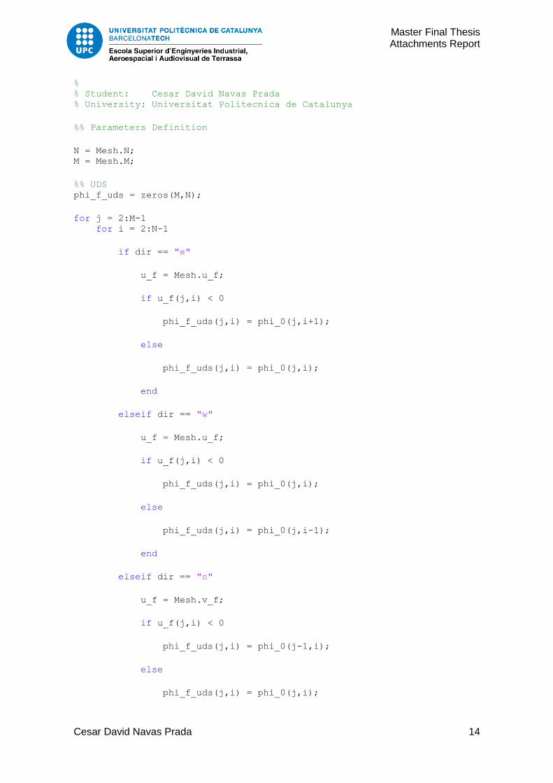
function [phi_f_uds] = UDS(Mesh,phi_0,dir) % UDS: Finds phi at the desired horizontal face for low resolution

scheme (upwind) % % INPUTS: % - Mesh: N [#] Number of nodes in axis X % M [#] Number of nodes in axis Y % u_f [m/s] Face's velocity in direction X % v_f [m/s] Face's velocity in direction Y % - phi_0: Phi (Pressure) in the prior time-step % - dir: Face where the value of phi is desired % % OUTPUTS: % - phi_f_uds: Phi of low resolution scheme (upwind) at the evaluated

face



% % Student: Cesar David Navas Prada % University: Universitat Politecnica de Catalunya



%% UDS phi_f_uds = zeros(M,N);

for j = 2:M-1 for i = 2:N-1

if dir == "e"

u_f = Mesh.u_f;

if u_f(j,i) < 0

phi_f_uds(j,i) = phi_0(j,i+1);

else

phi_f_uds(j,i) = phi_0(j,i);

end

elseif dir == "w"

u_f = Mesh.u_f;

if u_f(j,i) < 0


else

phi_f_uds(j,i) = phi_0(j,i-1);

end

elseif dir == "n"

u_f = Mesh.v_f;

if u_f(j,i) < 0

phi_f_uds(j,i) = phi_0(j-1,i);

else




end

elseif dir == "s"

u_f = Mesh.v_f;

if u_f(j,i) < 0


else

phi_f_uds(j,i) = phi_0(j+1,i);

end

else

error("Choose the correct direction")

end end end

2.1.2. Numerical Solvers

2.1.2.1. Point-by-Point

function [phi]=solvphi_pbp(Mesh,Coeff,phi_0) % solvphi_pbp: Solves the set of equations to find phi using % point-by-point method % % INPUTS: % - Mesh: N [#] Total nodes in axis X % M [#] Total nodes in axis Y % - Coeff: A_e Coefficient east node % A_w Coefficient west node % A_n Coefficient north node % A_s Coefficient south node % A_p Coefficient center node % b Resultant coefficient % - phi_0: Phi in the prior time-step % % OUTPUTS: % - phi [Pa]: Variable % % Student: Cesar David Navas Prada % University: Universitat Politecnica de Catalunya

%% Parameter Definiton




A_e = Coeff.A_e; A_w = Coeff.A_w; A_n = Coeff.A_n; A_s = Coeff.A_s; A_p = Coeff.A_p; b = Coeff.b;

%% Solver phi = zeros(M,N);

% Middle Nodes

phi(2:M-1,2:N-1) = (A_e(2:M-1,2:N-1).*phi_0(2:M-1,(2:N-1)+1) + A_w(2:M-

1,2:N-1).*phi_0(2:M-1,(2:N-1)-1)... + A_n(2:M-1,2:N-1).*phi_0((2:M-1)-1,2:N-1) + A_s(2:M-

1,2:N-1).*phi_0((2:M-1)+1,2:N-1)... + b(2:M-1,2:N-1))./(A_p(2:M-1,2:N-1));

% West Nodes

phi(1,1) = (A_e(1,1)*phi_0(1,2) + A_s(1,1).*phi_0(2,1) +

b(1,1))./(A_p(1,1)); phi(M,1) = (A_e(M,1)*phi_0(M,2) + A_n(M,1).*phi_0(M-1,1) +

b(M,1))./(A_p(M,1)); phi(2:M-1,1) = (A_e(2:M-1,1).*phi_0(2:M-1,2) + A_n(2:M-1,1).*phi_0((2:M-

1)-1,1)... + A_s(2:M-1,1).*phi_0((2:M-1)+1,1) + b(2:M-

1,1))./(A_p(2:M-1,1));

% East Nodes

phi(1,N) = (A_w(1,N).*phi_0(1,N-1) + A_s(1,N).*phi_0(2,N) +

b(1,N))./(A_p(1,N)); phi(M,N) = (A_w(M,N).*phi_0(M,N-1) + A_n(M,N).*phi_0(M-1,N) +

b(M,N))./(A_p(M,N)); phi(2:M-1,N) = (A_w(2:M-1,N).*phi_0(2:M-1,N-1) + A_n(2:M-

1,N).*phi_0((2:M-1)-1,N)... + A_s(2:M-1,N).*phi_0((2:M-1)+1,N) + b(2:M-

1,N))./(A_p(2:M-1,N));

% North Nodes

phi(1,2:N-1) = (A_e(1,2:N-1).*phi_0(1,(2:N-1)+1) + A_w(1,2:N-

1).*phi_0(1,(2:N-1)+1)... + A_s(1,2:N-1).*phi_0(2,2:N-1) + b(1,2:N-1))./(A_p(1,2:N-

1));

% South Nodes

phi(M,2:N-1) = (A_e(M,2:N-1).*phi_0(M,(2:N-1)+1) + A_w(M,2:N-

1).*phi_0(M,(2:N-1)+1)... + A_n(M,2:N-1).*phi_0(M-1,2:N-1) + b(M,2:N-

1))./(A_p(M,2:N-1));

2.1.2.2. Line-by-line



function [phi]=solvphi_lbl(Mesh,Coeff,phi_0) % solvphi_lbl: Solves the set of equations to find phi using % line-by-line method with a combination of rows and

columns % directions % % INPUTS: % - Mesh: N [#] Total nodes in axis X % M [#] Total nodes in axis Y % - Coeff: A_e Coefficient east node % A_w Coefficient west node % A_n Coefficient north node % A_s Coefficient south node % A_p Coefficient center node % b Resultant coefficient % - phi_0: Phi in the prior time-step % % OUTPUTS: % - phi: Variable % % Student: Cesar David Navas Prada % University: Universitat Politecnica de Catalunya



A_e = Coeff.A_e; A_w = Coeff.A_w; A_n = Coeff.A_n; A_s = Coeff.A_s; A_p = Coeff.A_p; b = Coeff.b;

%% ROWS (Left to Right) bs = zeros(M,N); P = zeros(M,N); Q = zeros(M,N); phi = zeros(M,N);

% West Nodes

bs(1,1) = A_s(1,1).*phi_0(2,1) + b(1,1); bs(M,1) = A_n(M,1).*phi_0(M-1,1) + b(M,1); bs(2:M-1,1) = A_n(2:M-1,1).*phi_0((2:M-1)-1,1)... + A_s(2:M-1,1).*phi_0((2:M-1)+1,1) + b(2:M-1,1);

P(1:M,1) = A_e(1:M,1)./A_p(1:M,1);

Q(1:M,1) = bs(1:M,1)./A_p(1:M,1);

phi(1:M,1) = P(1:M,1).*phi_0(1:M,2) + Q(1:M,1);

% Middle Nodes

bs(1,2:N-1) = A_s(1,2:N-1).*phi_0(2,2:N-1) + b(1,2:N-1); bs(M,2:N-1) = A_n(M,2:N-1).*phi_0(M-1,2:N-1) + b(M,2:N-1);



bs(2:M-1,2:N-1) = A_n(2:M-1,2:N-1).*phi_0((2:M-1)-1,2:N-1)... + A_s(2:M-1,2:N-1).*phi_0((2:M-1)+1,2:N-1) + b(2:M-

1,2:N-1);

for j = 1:M for i = 2:N-1

P(j,i) = A_e(j,i)/(A_p(j,i) - A_w(j,i)*P(j,i-1));

Q(j,i) = (bs(j,i) + A_w(j,i)*Q(j,i-1))/(A_p(j,i) -

A_w(j,i)*P(j,i-1));

end end

phi(1:M,2:N-1) = P(1:M,2:N-1).*phi_0(1:M,(2:N-1)+1) + Q(1:M,2:N-1);

% East Nodes

bs(1,N) = A_s(1,N).*phi_0(2,N) + b(1,N); bs(M,N) = A_n(M,N).*phi_0(M-1,N) + b(M,N); bs(2:M-1,N) = A_n(2:M-1,N).*phi_0((2:M-1)-1,N)... + A_s(2:M-1,N).*phi_0((2:M-1)+1,N) + b(2:M-1,N);

P(1:M,N) = 0;

Q(1:M,N) = (bs(1:M,N) + A_w(1:M,N).*Q(1:M,N-1))./(A_p(1:M,N)... - A_w(1:M,N).*P(1:M,N-

1));

phi(1:M,N) = Q(1:M,N);

%% COLUMNS (Up to Down) phi_0 = phi;

% North Nodes

bs(1,1) = A_e(1,1).*phi_0(1,2) + b(1,1); bs(1,N) = A_w(1,N).*phi_0(1,N-1) + b(1,N); bs(1,2:N-1) = A_e(1,2:N-1).*phi_0(1,(2:N-1)+1)... + A_w(1,2:N-1).*phi_0(1,(2:N-1)-1) + b(1,2:N-1);

P(1,1:N) = A_s(1,1:N)./A_p(1,1:N);

Q(1,1:N) = bs(1,1:N)./A_p(1,1:N);

phi(1,1:N) = P(1,1:N).*phi_0(2,1:N) + Q(1,1:N);

% Middle Nodes

bs(2:M-1,1) = A_e(2:M-1,1).*phi_0(2:M-1,2) + b(2:M-1,1); bs(2:M-1,N) = A_w(2:M-1,N).*phi_0(2:M-1,N-1) + b(2:M-1,N); bs(2:M-1,2:N-1) = A_e(2:M-1,2:N-1).*phi_0(2:M-1,(2:N-1)+1)... + A_w(2:M-1,2:N-1).*phi_0(2:M-1,(2:N-1)-1) + b(2:M-

1,2:N-1);



for i = 1:N for j = 2:M-1

P(j,i) = A_s(j,i)/(A_p(j,i) - A_n(j,i)*P(j-1,i));

Q(j,i) = (bs(j,i) + A_n(j,i)*Q(j-1,i))/(A_p(j,i) - A_n(j,i)*P(j-

1,i));

end end

phi(2:M-1,1:N) = P(2:M-1,1:N).*phi_0((2:M-1)+1,1:N) + Q(2:M-1,1:N);

% South Nodes

bs(M,1) = A_e(M,1).*phi_0(M,2) + b(M,1); bs(M,N) = A_w(M,N).*phi_0(M,N-1) + b(M,N); bs(M,2:N-1) = A_e(M,2:N-1).*phi_0(M,(2:N-1)+1)... + A_w(M,2:N-1).*phi_0(M,(2:N-1)-1) + b(M,2:N-1);

P(M,1:N) = 0;

Q(M,1:N) = (bs(M,1:N) + A_n(M,1:N).*Q(M-1,1:N))./(A_p(M,1:N)... - A_n(M,1:N).*P(M-

1,1:N));

phi(M,1:N) = Q(M,1:N);

2.1.3. Diagonal Flow

2.1.3.1. Main Code

clear close all

%%%%%%%%%%%%%%%%%%%%%%%%%%%%%%%%%%%%%%%%%%%%%%% %%%%%%%%%%%%%%% DIAGONAL FLOW %%%%%%%%%%%%%%% %%%%%%%%%% Cesar David Navas Prada %%%%%%%%%% %%%%%%%%%%%%%%%% MAIN SCRIPT %%%%%%%%%%%%%%%% %%%%%%%%%%%%%%%%%%%%%%%%%%%%%%%%%%%%%%%%%%%%%%%

%% Input Parameters

Data.L = 1; % [m] length in axis X Data.H = 1; % [m] Hight in axis Y Data.d_t = 0.01; % [s] Time Step Data.V0 = 1; % [m/s] Initial velocity Data.alpha = 45*pi/180; % [Radian] Angle for wall conditions rho_gamma = [10 1e3 1e6]; % Ratio density/diffusive coefficient gamma = 1; % Diffusive coefficient rho = rho_gamma*gamma; % [Kg/m^3] Density Data.sc = "upwind"; % Numerical Scheme ( upwind, upwind2, quick,

fromm, smart)



%% Mesh

Mesh = mesh(Data,50,50);

%% Iteration

error = 1e-3; % Convergence Criteria

phi_ds = zeros(length(rho_gamma),Mesh.M); T_time = zeros(1,length(rho_gamma));

for i = 1:length(rho_gamma)

tic phi_0 = zeros(Mesh.M,Mesh.N); Error = zeros; Time = zeros; phi_1 = phi_0; diff_0 = inf; z = 0;

% Function to find constant coefficients C_Coeff = C_coeff(Mesh,Data,gamma,rho(i));

% Solver while diff_0 > error

% Function to find time-dependent coefficients Coeff = T_coeff(Mesh,Data,C_Coeff,gamma,rho(i),phi_0,z);

z = z + 1; diff_1 = inf;

while diff_1 > error

% Solver function (p-b-p or l-b-l) phi = solvphi_pbp(Mesh,Coeff,phi_1);

sub_1 = abs(phi_1 - phi); diff_1 = max(sub_1(:)); phi_1 = phi;

end

sub_0 = abs(phi_0 - phi); diff_0 = max(sub_0(:)/Data.d_t); Time(z) = floor(toc); phi_0 = phi; fprintf('Rho/gamma %d ; Error = %d ; Iteration

%d\n',rho(i),diff_0,z) Error(z) = diff_0;

end

X = Mesh.X; Y = Mesh.Y; M = Mesh.M;



% Error and iterations figure subplot(2,1,1) plot(1:z,Error) xlabel('Iteration n°','Fontsize',12) ylabel('Error |\phi - \phi^*|/\Deltat','Fontsize',16) axis([0 inf 0 20])

if i == 1 title('\rho/\Gamma=10','Fontsize',18) elseif i == 2 title('\rho/\Gamma=10^3','Fontsize',18) else title('\rho/\Gamma=10^6','Fontsize',18) end

subplot(2,1,2) plot(Time,Error) xlabel('Time [s]','Fontsize',12) ylabel('Error |\phi - \phi^*|/\Deltat','Fontsize',16) axis([0 inf 0 20])

%Position desired for j = 1:M

phi_ds(i,j) = phi(j,j); % Vector to evaluate phi

end

% Graphic of phi in the domain figure; contourf(X(1,:),Y(:,1),phi,'LineStyle','none','LevelStep',0.01); xlabel('x [m]','Fontsize',18) ylabel('y [m]','Fontsize',18)


colorbar

T_time(i) = max(Time);

end

%% Plotting

% Plot graphic for x desired at different rho/gamma figure; color = {'b' 'r' 'g'};




plot(X(M,:),phi_ds(i,:),color{i}) hold on

end

xlabel('X','Fontsize',18) ylabel('\phi','Fontsize',18) legend('\rho/\Gamma=10','\rho/\Gamma=10^3','\rho/\Gamma=10^6','Location'

,'Best') axis([0 1 0 1])

%% Time of convergence

fprintf('Time of convergence rho/gamma = 10 is %d [s]\n',T_time(1)) fprintf('Time of convergence rho/gamma = 10^3 is %d [s]\n',T_time(2)) fprintf('Time of convergence rho/gamma = 10^6 is %d [s]\n',T_time(3)) fprintf('Total time is %d [s]\n',sum(T_time))

2.1.3.2. Mesh Code

function [Mesh] = mesh(Data,n,m) % mesh: Creates a node-centered and structured mesh for a % 2D case with dimensions (L by H) and (n by m) number of control % volumes % % INPUTS: % - Data: L [m] Length in Axis X % H [m] Height in Axis Y % V0 [m/s] Initial velocity % alpha [degree] Angle for wall conditions % - n [#] Control volumes in axis X % - m [#] Control volumes in axis Y % % OUTPUTS: % - Mesh: N [#] Number of nodes in axis X % M [#] Number of nodes in axis Y % n [#] Control volumes in axis X % m [#] Control volumes in axis Y % dx [m] Control volume's Lenght (X) % dy [m] Control volume's Height (Y) % X [m] Nodes' position in axis X % Y [m] Nodes' position in axis Y % X_f [m] Faces' position in axis X % Y_f [m] Faces' position in axis Y % u [m/s] Node's velocity in direction X % v [m/s] Node's velocity in direction Y % u_f [m/s] Face's velocity in direction X % v_f [m/s] Face's velocity in direction Y % DeltaX [m] Control volume's length (X) % DeltaY [m] Control volume's Height (Y) % deltaX [m] Central node's distances (X) % deltaY [m] Central node's distances (Y) % % Case: DIAGONAL FLOW % Student: Cesar David Navas Prada



% University: Universitat Politecnica de Catalunya


L = Data.L; H = Data.H; V0 = Data.V0; alpha = Data.alpha;

%% Geometry of the mesh

dx = L/n; % Control volume's Lenght (X) dy = H/m; % Control volume's Height (Y)

%% Number of nodes

N = n + 2; % Number of nodes in axis X M = m + 2; % Number of nodes in axis Y

%% Node's position X = zeros(M,N); Y = zeros(M,N);

% Axis X X(1:M,1) = 0; X(1:M,2) = X(1:M,1) + dx/2;


X(j,i) = X(j,i-1) + dx;

end end

X(1:M,N) = X(1:M,N-1) + dx/2;

% Axis Y Y(1,1:N) = H; Y(2,1:N) = Y(1,1:N) - dy/2;


Y(j,i) = Y(j-1,i) - dy;

end end

Y(M,1:N) = Y(M-1,1:N) - dy/2;

%% Face's position X_f = zeros(M+1,N+1); Y_f = zeros(M+1,N+1);

% Axis X



X_f(1:M+1,1) = 0; X_f(1:M+1,2) = X_f(1:M+1,1) + dx/2; X_f(1:M+1,3) = X_f(1:M+1,2) + dx/2;

for j = 1:M+1 for i = 4:N-1

X_f(j,i) = X_f(j,i-1) + dx;

end end

X_f(1:M+1,N) = X_f(1:M+1,N-1) + dx/2; X_f(1:M+1,N+1) = X_f(1:M+1,N) + dx/2;

% Axis Y Y_f(1,1:N+1) = H; Y_f(2,1:N+1) = Y_f(1,1:N+1) - dy/2; Y_f(3,1:N+1) = Y_f(2,1:N+1) - dy/2;

for i = 1:N+1 for j = 4:M-1

Y_f(j,i) = Y_f(j-1,i) - dy;

end end

Y_f(M,1:N+1) = Y_f(M-1,1:N+1) - dy/2; Y_f(M+1,1:N+1) = Y_f(M,1:N+1) - dy/2;

%% Control Volume's length DeltaX = zeros(M,N); DeltaY = zeros(M,N);

% Delta X for j = 1:M for i = 1:N

if i == 2

DeltaX(j,i) = X_f(j,i+1) - X_f(j,i-1);

elseif i == N-1

DeltaX(j,i) = X_f(j,i+2) - X_f(j,i);

else


end

end end



% Delta Y for i = 1:N for j = 1:M

if j == 2

DeltaY(j,i) = Y_f(j-1,i) - Y_f(j+1,i);

elseif j == M-1

DeltaY(j,i) = Y_f(j,i) - Y_f(j+2,i);

else


end

end end

%% Node's distance deltaX = zeros(M,N,2); deltaY = zeros(M,N,2);

% delta X for j = 1:M for i = 1:N

if i == 1

deltaX(j,i,1) = X(j,i+1) - X(j,i); % East deltaX(j,i,2) = 0; % West

elseif i == N

deltaX(j,i,1) = 0; % East deltaX(j,i,2) = X(j,i) - X(j,i-1); % West

else

deltaX(j,i,1) = X(j,i+1) - X(j,i); % East deltaX(j,i,2) = X(j,i) - X(j,i-1); % West

end

end end

% delta Y for i = 1:N for j = 1:M

if j == 1

deltaY(j,i,1) = 0; % North



deltaY(j,i,2) = Y(j,i) - Y(j+1,i); % South

elseif j == M

deltaY(j,i,1) = Y(j-1,i) - Y(j,i); % North deltaY(j,i,2) = 0; % South

else

deltaY(j,i,1) = Y(j-1,i) - Y(j,i); % North deltaY(j,i,2) = Y(j,i) - Y(j+1,i); % South

end

end end

%% Node's velocity u = zeros(M,N); v = zeros(M,N);

u(1:M,1:N) = vel_Diagonal(V0,alpha,"x"); v(1:M,1:N) = vel_Diagonal(V0,alpha,"y");

%% Face's velocity u_f = zeros(M,N); v_f = zeros(M,N);

u_f(1:M,1:N) = vel_Diagonal(V0,alpha,"x"); v_f(1:M,1:N) = vel_Diagonal(V0,alpha,"y");

%% Mesh Structure setup

Mesh.N = N; Mesh.M = M; Mesh.n = n; Mesh.m = m; Mesh.dx = dx; Mesh.dy = dy; Mesh.X = X; Mesh.Y = Y; Mesh.X_f = X_f; Mesh.Y_f = Y_f; Mesh.u = u; Mesh.v = v; Mesh.u_f = u_f; Mesh.v_f = v_f; Mesh.DeltaX = DeltaX; Mesh.DeltaY = DeltaY; Mesh.deltaX = deltaX; Mesh.deltaY = deltaY;



2.1.3.3. Velocity Field Code

function [vel] = vel_Diagonal(V0,alpha,dir) %vel_Diagonal: Finds the velocity field at each node and face

exclusively % for the Diagonal Flow case % % INPUTS: % - V0 [m/s]: Initial velocity % - alpha [Radian]: Wall condition's angle % - dir: Face where the value of phi is desired % % OUTPUTS: % - vel : Velocity at node or face % % Case: DIAGONAL FLOW % Student: Cesar David Navas Prada % University: Universitat Politecnica de Catalunya

%% Velocity

if dir == "x"

vel = V0*cos(alpha);

elseif dir == "y"

vel = V0*sin(alpha);

else

error("choose the correct direction")

end

2.1.3.4. Coefficients Code

function [C_Coeff] = C_coeff(Mesh,Data,gamma,rho) % C_coeff: Finds the non time-dependent (Constant) coefficients for the % given parameters at each node in the main mesh % % INPUTS: % - Mesh: N [#] Number of nodes in axis X % M [#] Number of nodes in axis Y % DeltaX [m] Control volume's length (X) % DeltaY [m] Control volume's Height (Y) % deltaX [m] Central node's distances (X) % deltaY [m] Central node's distances (Y) % - Data: alpha [Radian] Wall condition's angle % V0 [m/s] Initial velocity % - gamma : Diffusion coefficient % - rho : [Kg/m^3] Fluid's Density %



% OUTPUTS: % - C_Coeff: A_e Coefficient east node % A_w Coefficient west node % A_n Coefficient north node % A_s Coefficient south node % A_p Coefficient center node % A_p0 Coefficient time-step % b Resultant coefficient % b_dc Coefficient deferred correction % Fe Flow rate east face % Fw Flow rate west face % Fn Flow rate north face % Fs Flow rate south face % % Case: DIAGONAL FLOW % Student: Cesar David Navas Prada % University: Universitat Politecnica de Catalunya

%% Paremeters Definition

N = Mesh.N; M = Mesh.M; DeltaX = Mesh.DeltaX; DeltaY = Mesh.DeltaY; deltaX = Mesh.deltaX; deltaY = Mesh.deltaY;

alpha = Data.alpha; V0 = Data.V0;

%% Wall coefficients A_e = zeros(M,N); A_w = zeros(M,N); A_n = zeros(M,N); A_s = zeros(M,N); A_p = zeros(M,N); A_p0 = zeros(M,N); b = zeros(M,N); b_dc = zeros(M,N);

% West Nodes A_e(2:M-1,1) = 0; A_w(2:M-1,1) = 0; A_n(2:M-1,1) = 0; A_s(2:M-1,1) = 0; A_p(2:M-1,1) = 1; b(2:M-1,1) = 1;

% East Nodes A_e(2:M-1,N) = 0; A_w(2:M-1,N) = 1; A_n(2:M-1,N) = 0; A_s(2:M-1,N) = 0; A_p(2:M-1,N) = 1; b(2:M-1,N) = 0;

% North Nodes A_e(1,2:N-1) = 0; A_w(1,2:N-1) = 0;



A_n(1,2:N-1) = 0; A_s(1,2:N-1) = 1; A_p(1,2:N-1) = 1; b(1,2:N-1) = 0;

% South Nodes A_e(M,2:N-1) = 0; A_w(M,2:N-1) = 0; A_n(M,2:N-1) = 0; A_s(M,2:N-1) = 0; A_p(M,2:N-1) = 1; b(M,2:N-1) = 0;

%% Middle Nodes De = zeros(M,N); Dw = zeros(M,N); Dn = zeros(M,N); Ds = zeros(M,N); Fe = zeros(M,N); Fw = zeros(M,N); Fn = zeros(M,N); Fs = zeros(M,N);

De(2:M-1,2:N-1) = (DeltaY(2:M-1,2:N-1))./(deltaX(2:M-1,2:N-1,1));

% Conductance east nodes Fe(2:M-1,2:N-1) = (rho/gamma)*(vel_Diagonal(V0,alpha,"x"))*(DeltaY(2:M-

1,2:N-1)); % Flow rate east nodes

Dw(2:M-1,2:N-1) = (DeltaY(2:M-1,2:N-1))./(deltaX(2:M-1,2:N-1,2));

% Conductance west nodes Fw(2:M-1,2:N-1) = (rho/gamma)*(vel_Diagonal(V0,alpha,"x"))*(DeltaY(2:M-

1,2:N-1)); % Flow rate west nodes

Dn(2:M-1,2:N-1) = (DeltaX(2:M-1,2:N-1))./(deltaY(2:M-1,2:N-1,1));

% Conductance north nodes Fn(2:M-1,2:N-1) = (rho/gamma)*(vel_Diagonal(V0,alpha,"y"))*(DeltaX(2:M-

1,2:N-1)); % Flow rate north nodes

Ds(2:M-1,2:N-1) = (DeltaX(2:M-1,2:N-1))./(deltaY(2:M-1,2:N-1,2));

% Conductance south nodes Fs(2:M-1,2:N-1) = (rho/gamma)*(vel_Diagonal(V0,alpha,"y"))*(DeltaX(2:M-

1,2:N-1)); % Flow rate south nodes

for j = 2:M-1 for i = 2:N-1

A_e(j,i) = De(j,i) + max(-Fe(j,i), 0); A_w(j,i) = Dw(j,i) + max(Fw(j,i), 0); A_n(j,i) = Dn(j,i) + max(-Fn(j,i), 0); A_s(j,i) = Ds(j,i) + max(Fs(j,i), 0);

end end

%% Corner nodes

% West - Top A_e(1,1) = 0.5;



A_w(1,1) = 0; A_n(1,1) = 0; A_s(1,1) = 0.5; A_p(1,1) = 1; b(1,1) = 0;

% East - Top A_e(1,N) = 0; A_w(1,N) = 0.5; A_n(1,N) = 0; A_s(1,N) = 0.5; A_p(1,N) = 1; b(1,N) = 0;

% West - Bottom A_e(M,1) = 0.5; A_w(M,1) = 0; A_n(M,1) = 0.5; A_s(M,1) = 0; A_p(M,1) = 1; b(M,1) = 0;

% East - Bottom A_e(M,N) = 0; A_w(M,N) = 0.5; A_n(M,N) = 0.5; A_s(M,N) = 0; A_p(M,N) = 1; b(M,N) = 0;

%% C_Coeff structure setup

C_Coeff.A_e = A_e; C_Coeff.A_w = A_w; C_Coeff.A_n = A_n; C_Coeff.A_s = A_s; C_Coeff.A_p = A_p; C_Coeff.A_p0 = A_p0; C_Coeff.b = b; C_Coeff.b_dc = b_dc; C_Coeff.Fe = Fe; C_Coeff.Fw = Fw; C_Coeff.Fn = Fn; C_Coeff.Fs = Fs;

function [Coeff] = T_coeff(Mesh,Data,C_Coeff,gamma,rho,phi_0,z) % T_coeff: Finds the time-dependent coefficients for the % given parameters at each node in the main mesh % % INPUTS: % - Mesh: N [#] Number of nodes in axis X % M [#] Number of nodes in axis Y % DeltaX [m] Control volume's length (X) % DeltaY [m] Control volume's Height (Y) % - Data: d_t [s] Time Step % sc Numerical Scheme (upwind, upwind2, quick, fromm, smart)



% - C_Coeff: A_e Coefficient east node % A_w Coefficient west node % A_n Coefficient north node % A_s Coefficient south node % A_p Coefficient center node % A_p0 Coefficient time-step % b Resultant coefficient % b_dc Coefficient deferred correction % Fe Flow rate east face % Fw Flow rate west face % Fn Flow rate north face % Fs Flow rate south face % - gamma : Diffusion coefficient % - rho : [Kg/m^3] Fluid's Density % - phi_0: Phi in a prior time-step % - z: Countant parameter % % OUTPUTS: % - Coeff: A_e Coefficient east node % A_w Coefficient west node % A_n Coefficient north node % A_s Coefficient south node % A_p Coefficient center node % A_p0 Coefficient time-step % b Resultant coefficient % % Case: DIAGONAL FLOW % Student: Cesar David Navas Prada % University: Universitat Politecnica de Catalunya


N = Mesh.N; M = Mesh.M; DeltaX = Mesh.DeltaX; DeltaY = Mesh.DeltaY;

d_t = Data.d_t; sc = Data.sc;

A_e = C_Coeff.A_e; A_w = C_Coeff.A_w; A_n = C_Coeff.A_n; A_s = C_Coeff.A_s; A_p = C_Coeff.A_p; A_p0 = C_Coeff.A_p0; b = C_Coeff.b; b_dc = C_Coeff.b_dc;

Fe = C_Coeff.Fe; Fw = C_Coeff.Fw; Fn = C_Coeff.Fn; Fs = C_Coeff.Fs;

%% Middle Nodes

if z == 0



phi_e_hrs = zeros(M-1,N-1); phi_e_uds = zeros(M-1,N-1);

phi_w_hrs = zeros(M-1,N-1); phi_w_uds = zeros(M-1,N-1);

phi_n_hrs = zeros(M-1,N-1); phi_n_uds = zeros(M-1,N-1);

phi_s_hrs = zeros(M-1,N-1); phi_s_uds = zeros(M-1,N-1);

else

phi_e_hrs = HRS(Mesh,phi_0,sc,"e"); phi_e_uds = UDS(Mesh,phi_0,"e");

phi_w_hrs = HRS(Mesh,phi_0,sc,"w"); phi_w_uds = UDS(Mesh,phi_0,"w");

phi_n_hrs = HRS(Mesh,phi_0,sc,"n"); phi_n_uds = UDS(Mesh,phi_0,"n");

phi_s_hrs = HRS(Mesh,phi_0,sc,"s"); phi_s_uds = UDS(Mesh,phi_0,"s");

end

A_p0(2:M-1,2:N-1) = ((rho/gamma)*(DeltaX(2:M-1,2:N-1)).*(DeltaY(2:M-

1,2:N-1)))/(d_t); A_p(2:M-1,2:N-1) = A_e(2:M-1,2:N-1) + A_w(2:M-1,2:N-1) + A_n(2:M-1,2:N-

1) + A_s(2:M-1,2:N-1) + A_p0(2:M-1,2:N-1);

b_dc(3:M-2,3:N-2) = -Fe(3:M-2,3:N-2).*(phi_e_hrs(3:M-2,3:N-2) -

phi_e_uds(3:M-2,3:N-2))... + Fw(3:M-2,3:N-2).*(phi_w_hrs(3:M-2,3:N-2) -

phi_w_uds(3:M-2,3:N-2))... - Fn(3:M-2,3:N-2).*(phi_n_hrs(3:M-2,3:N-2) -

phi_n_uds(3:M-2,3:N-2))... + Fs(3:M-2,3:N-2).*(phi_s_hrs(3:M-2,3:N-2) -

phi_s_uds(3:M-2,3:N-2));

b(2:M-1,2:N-1)= b_dc(2:M-1,2:N-1) + A_p0(2:M-1,2:N-1).*phi_0(2:M-1,2:N-

1);

%% Coeff structure setup

Coeff.A_e = A_e; Coeff.A_w = A_w; Coeff.A_n = A_n; Coeff.A_s = A_s; Coeff.A_p = A_p; Coeff.A_p0 = A_p0; Coeff.b = b;



2.1.4. Smith-Hutton Problem

2.1.4.1. Main Code

clear close all

%%%%%%%%%%%%%%%%%%%%%%%%%%%%%%%%%%%%%%%%%%%%%%% %%%%%%%%%%%%%%% SMITH-HUTTON %%%%%%%%%%%%%%% %%%%%%%%%% Cesar David Navas Prada %%%%%%%%%% %%%%%%%%%%%%%%%% MAIN SCRIPT %%%%%%%%%%%%%%%% %%%%%%%%%%%%%%%%%%%%%%%%%%%%%%%%%%%%%%%%%%%%%%%

%% Input Parameters

Data.L = 2; % [m] length in axis X Data.H = 1; % [m] Hight in axis Y Data.d_t = 0.1; % [s] Time Step Data.alpha = 10; % [degree] Angle for wall conditions rho_gamma = [10 1e3 1e6]; % Ratio density/diffusive coefficient gamma = 1; % Diffusive coefficient rho = rho_gamma*gamma; % [Kg/m^3] Density Data.sc = "upwind"; % Numerical Scheme ( upwind, upwind2,

quick, fromm, smart)

%% Mesh

Mesh = mesh(Data,100,50);

%% Iteration

error = 1e-5; % Convergence Criteria

phi_ds {length(rho_gamma)} = zeros; T_time = zeros(1,length(rho_gamma));


tic phi_0 = zeros(Mesh.M,Mesh.N); Error = zeros; Time = zeros; phi_1 = phi_0; diff_0 = inf; z = 0;

% Function to find constant coefficients C_Coeff = C_coeff(Mesh,Data,gamma,rho(i));

% Solver while diff_0 > error

% Function to find time-dependent coefficients Coeff = T_coeff(Mesh,Data,C_Coeff,gamma,rho(i),phi_0,z);



z = z + 1; diff_1 = inf;

while diff_1 > error

% Solver function (p-b-p or l-b-l) phi = solvphi_lbl(Mesh,Coeff,phi_1);

sub_1 = abs(phi_1 - phi); diff_1 = max(sub_1(:)); phi_1 = phi;

end

sub_0 = abs(phi_0 - phi); diff_0 = max(sub_0(:)/Data.d_t); Time(z) = floor(toc); phi_0 = phi; fprintf('Rho/gamma %d ; Error = %d ; Iteration

%d\n',rho(i),diff_0,z) Error(z) = diff_0;

end

X = Mesh.X; Y = Mesh.Y; M = Mesh.M;

% Position desired x_ds = 0:0.01:Data.L/2; % Vector to evaluate phi phi_ds{i} = interp1(X(M,:),phi(M,:),x_ds); % Interpolation at X desired

% Error and iterations figure subplot(2,1,1) plot(1:z,Error) xlabel('Iteration n°','Fontsize',12) ylabel('Error |\phi - \phi^*|/\Deltat','Fontsize',16) axis([0 inf 0 20])


subplot(2,1,2) plot(Time,Error) xlabel('Time [s]','Fontsize',12) ylabel('Error |\phi - \phi^*|/\Deltat','Fontsize',16) axis([0 inf 0 20])

%Graphic of phi in the domain figure; contourf(X(1,:),Y(:,1),phi,'LineStyle','none','LevelStep',0.01); xlabel('x [m]','Fontsize',18)



ylabel('y [m]','Fontsize',18)


colorbar

T_time(i) = max(Time);

end

%% Plotting

% Plot graphic for x desired at different rho/gamma figure; color = {'b' 'r' 'g'}; for i = 1:length(rho_gamma)

plot(x_ds,phi_ds{i},color{i}) hold on

end xlabel('X','Fontsize',18) ylabel('\phi','Fontsize',18) legend('\rho/\Gamma=10','\rho/\Gamma=10^3','\rho/\Gamma=10^6','Location'

,'Best')

%% Saving file

fileID = fopen('Smith-Hutton_CDNP.txt','w'); %Save the file with

the required data fprintf(fileID,'%s %s %s %s\n',' X ',' rho/gamma=10','

rho/gamma=10^3',' rho/gamma=10^6'); fprintf(fileID,'%.6f\t %.6f\t\t %.6f\t\t

%.6f\n',[x_ds;phi_ds{1};phi_ds{2};phi_ds{3}]); fclose(fileID);

%% Time of convergence

fprintf('Time of convergence rho/gamma = 10 is %d [s]\n',T_time(1)) fprintf('Time of convergence rho/gamma = 10^3 is %d [s]\n',T_time(2)) fprintf('Time of convergence rho/gamma = 10^6 is %d [s]\n',T_time(3)) fprintf('Total time is %d [s]\n',sum(T_time))

2.1.4.2. Mesh Code

function [Mesh] = mesh(Data,n,m) % mesh: Creates a node-centered and structured mesh for a % 2D case with dimensions (L by H) and (n by m) number of control



% volumes % % INPUTS: % - Data: L [m] Length in Axis X % H [m] Height in Axis Y % - n [#] Control volumes in axis X % - m [#] Control volumes in axis Y % % OUTPUTS: % - Mesh: N [#] Number of nodes in axis X % M [#] Number of nodes in axis Y % n [#] Control volumes in axis X % m [#] Control volumes in axis Y % dx [m] Control volume's Lenght (X) % dy [m] Control volume's Height (Y) % X [m] Nodes' position in axis X % Y [m] Nodes' position in axis Y % X_f [m] Faces' position in axis X % Y_f [m] Faces' position in axis Y % u [m/s] Node's velocity in direction X % v [m/s] Node's velocity in direction Y % u_f [m/s] Face's velocity in direction X % v_f [m/s] Face's velocity in direction Y % DeltaX [m] Control volume's length (X) % DeltaY [m] Control volume's Height (Y) % deltaX [m] Central node's distances (X) % deltaY [m] Central node's distances (Y) % % Case: SMITH-HUTTON % Student: Cesar David Navas Prada % University: Universitat Politecnica de Catalunya


L = Data.L; H = Data.H;


dx = L/n; % Control volume's Lenght (X) dy = H/m; % Control volume's Height (Y)

%% Number of nodes

N = n + 2; %Number of nodes in axis X M = m + 2; %Number of nodes in axis Y


% Axis X X(1:M,1) = -L/2; X(1:M,2) = X(1:M,1) + dx/2;




X(j,i) = X(j,i-1) + dx;

end end

X(1:M,N) = X(1:M,N-1) + dx/2;

% Axis Y Y(1,1:N) = H; Y(2,1:N) = Y(1,1:N) - dy/2;


Y(j,i) = Y(j-1,i) - dy;

end end

Y(M,1:N) = Y(M-1,1:N) - dy/2;

%% Face's position X_f = zeros(M+1,N+1); Y_f = zeros(M+1,N+1);

% Axis X

X_f(1:M+1,1) = -L/2; X_f(1:M+1,2) = X_f(1:M+1,1) + dx/2; X_f(1:M+1,3) = X_f(1:M+1,2) + dx/2;

for j = 1:M+1 for i = 4:N-1

X_f(j,i) = X_f(j,i-1) + dx;

end end

X_f(1:M+1,N) = X_f(1:M+1,N-1) + dx/2; X_f(1:M+1,N+1) = X_f(1:M+1,N) + dx/2;

% Axis Y Y_f(1,1:N+1) = H; Y_f(2,1:N+1) = Y_f(1,1:N+1) - dy/2; Y_f(3,1:N+1) = Y_f(2,1:N+1) - dy/2;

for i = 1:N+1 for j = 4:M-1

Y_f(j,i) = Y_f(j-1,i) - dy;

end end

Y_f(M,1:N+1) = Y_f(M-1,1:N+1) - dy/2;



Y_f(M+1,1:N+1) = Y_f(M,1:N+1) - dy/2;



if i == 2

DeltaX(j,i) = X_f(j,i+1) - X_f(j,i-1);

elseif i == N-1


else


end

end end


if j == 2

DeltaY(j,i) = Y_f(j-1,i) - Y_f(j+1,i);

elseif j == M-1


else


end

end end





if i == 1

deltaX(j,i,1) = X(j,i+1) - X(j,i); % East deltaX(j,i,2) = 0; % West

elseif i == N

deltaX(j,i,1) = 0; % East deltaX(j,i,2) = X(j,i) - X(j,i-1); % West

else

deltaX(j,i,1) = X(j,i+1) - X(j,i); % East deltaX(j,i,2) = X(j,i) - X(j,i-1); % West

end

end end


if j == 1

deltaY(j,i,1) = 0; % North deltaY(j,i,2) = Y(j,i) - Y(j+1,i); % South

elseif j == M

deltaY(j,i,1) = Y(j-1,i) - Y(j,i); % North deltaY(j,i,2) = 0; % South

else

deltaY(j,i,1) = Y(j-1,i) - Y(j,i); % North deltaY(j,i,2) = Y(j,i) - Y(j+1,i); % South

end

end end

%% Node's velocity u = zeros(M,N); v = zeros(M,N);

u(1:M,1:N) = vel_SH(Y(1:M,1:N),X(1:M,1:N)); v(1:M,1:N) = vel_SH(-X(1:M,1:N),Y(1:M,1:N));

%% Face's velocity u_f = zeros(M,N); v_f = zeros(M,N);

u_f(1:M,1:N) = vel_SH(Y_f(1:M,1:N),X_f(1:M,1:N));



v_f(1:M,1:N) = vel_SH(-X_f(1:M,1:N),Y_f(1:M,1:N));

%% Mesh Structure setup

Mesh.N = N; Mesh.M = M; Mesh.n = n; Mesh.m = m; Mesh.dx = dx; Mesh.dy = dy; Mesh.X = X; Mesh.Y = Y; Mesh.X_f = X_f; Mesh.Y_f = Y_f; Mesh.u = u; Mesh.v = v; Mesh.u_f = u_f; Mesh.v_f = v_f; Mesh.DeltaX = DeltaX; Mesh.DeltaY = DeltaY; Mesh.deltaX = deltaX; Mesh.deltaY = deltaY;

2.1.4.3. Velocity Field Code

function [vel] = vel_SH(A,B) %vel_SH: Finds the velocity field at each node and face exclusively % for the Smith-Hutton case % % INPUTS: % - A: Single component A of the velocity field % - B: Squared component B of the velocity field % % OUTPUTS: % - vel : Velocity field % % Case: SMITH-HUTTON % Student: Cesar David Navas Prada % University: Universitat Politecnica de Catalunya

%% Velocity

vel = 2*A.*(1 - B.^2);


function [C_Coeff] = C_coeff(Mesh,Data,gamma,rho) % C_coeff: Finds the non time-dependent (Constant) coefficients for the % given parameters at each node in the main mesh % % INPUTS: % - Mesh: N [#] Number of nodes in axis X



% M [#] Number of nodes in axis Y % DeltaX [m] Control volume's length (X) % DeltaY [m] Control volume's Height (Y) % deltaX [m] Central node's distances (X) % deltaY [m] Central node's distances (Y) % u_f [m/s] Face's velocity in direction X % v_f [m/s] Face's velocity in direction Y % - Data: alpha [Radian] Wall condition's angle % - gamma : Diffusion coefficient % - rho : [Kg/m^3] Fluid's Density % % OUTPUTS: % - C_Coeff: A_e Coefficient east node % A_w Coefficient west node % A_n Coefficient north node % A_s Coefficient south node % A_p Coefficient center node % A_p0 Coefficient time-step % b Resultant coefficient % b_dc Coefficient deferred correction % Fe Flow rate east face % Fw Flow rate west face % Fn Flow rate north face % Fs Flow rate south face % % Case: SMITH-HUTTON % Student: Cesar David Navas Prada % University: Universitat Politecnica de Catalunya


N = Mesh.N; M = Mesh.M; X = Mesh.X; DeltaX = Mesh.DeltaX; DeltaY = Mesh.DeltaY; deltaX = Mesh.deltaX; deltaY = Mesh.deltaY; u_f = Mesh.u_f; v_f = Mesh.v_f;

alpha = Data.alpha;

%% Wall coefficients A_e = zeros(M,N); A_w = zeros(M,N); A_n = zeros(M,N); A_s = zeros(M,N); A_p = zeros(M,N); A_p0 = zeros(M,N); b = zeros(M,N); b_dc = zeros(M,N);

% West Nodes A_e(2:M-1,1) = 0; A_w(2:M-1,1) = 0; A_n(2:M-1,1) = 0; A_s(2:M-1,1) = 0; A_p(2:M-1,1) = 1;



b(2:M-1,1) = 1 - tanh(alpha);

% East Nodes A_e(2:M-1,N) = 0; A_w(2:M-1,N) = 0; A_n(2:M-1,N) = 0; A_s(2:M-1,N) = 0; A_p(2:M-1,N) = 1; b(2:M-1,N) = 1 - tanh(alpha);

% North Nodes A_e(1,2:N-1) = 0; A_w(1,2:N-1) = 0; A_n(1,2:N-1) = 0; A_s(1,2:N-1) = 0; A_p(1,2:N-1) = 1; b(1,2:N-1) = 1 - tanh(alpha);

% South Nodes

% INLET A_e(M,2:N/2) = 0; A_w(M,2:N/2) = 0; A_n(M,2:N/2) = 0; A_s(M,2:N/2) = 0; A_p(M,2:N/2) = 1; b(M,2:N/2) = 1 + tanh(alpha*(2*X(M,2:N/2) + 1));

% OUTLET A_e(M,(N/2)+1:N-1) = 0; A_w(M,(N/2)+1:N-1) = 0; A_n(M,(N/2)+1:N-1) = 1; A_s(M,(N/2)+1:N-1) = 0; A_p(M,(N/2)+1:N-1) = 1; b(M,(N/2)+1:N-1) = 0;

%% Middle nodes

De = zeros(M,N); Dw = zeros(M,N); Dn = zeros(M,N); Ds = zeros(M,N); Fe = zeros(M,N); Fw = zeros(M,N); Fn = zeros(M,N); Fs = zeros(M,N);

De(2:M-1,2:N-1) = (DeltaY(2:M-1,2:N-1))./(deltaX(2:M-1,2:N-1,1));

% Conductance east nodes Fe(2:M-1,2:N-1) = (rho/gamma)*(u_f(2:M-1,(2:N-1)+1)).*(DeltaY(2:M-1,2:N-

1)); % Flow rate east nodes

Dw(2:M-1,2:N-1) = (DeltaY(2:M-1,2:N-1))./(deltaX(2:M-1,2:N-1,2));

%Conductance west nodes Fw(2:M-1,2:N-1) = (rho/gamma)*(u_f(2:M-1,2:N-1)).*(DeltaY(2:M-1,2:N-1));

%Flow rate west nodes



Dn(2:M-1,2:N-1) = (DeltaX(2:M-1,2:N-1))./(deltaY(2:M-1,2:N-1,1));

%Conductance north nodes Fn(2:M-1,2:N-1) = (rho/gamma)*(v_f(2:M-1,2:N-1)).*(DeltaX(2:M-1,2:N-1));

%Flow rate north nodes

Ds(2:M-1,2:N-1) = (DeltaX(2:M-1,2:N-1))./(deltaY(2:M-1,2:N-1,2));

%Conductance south nodes Fs(2:M-1,2:N-1) = (rho/gamma)*(v_f((2:M-1)+1,2:N-1)).*(DeltaX(2:M-1,2:N-

1)); %Flow rate south nodes

for j = 2:M-1 for i = 2:N-1

A_e(j,i) = De(j,i) + max(-Fe(j,i), 0); A_w(j,i) = Dw(j,i) + max(Fw(j,i), 0); A_n(j,i) = Dn(j,i) + max(-Fn(j,i), 0); A_s(j,i) = Ds(j,i) + max(Fs(j,i), 0);

end end

%% Corner nodes

% West - Top A_e(1,1) = 0.5; A_w(1,1) = 0; A_n(1,1) = 0; A_s(1,1) = 0.5; A_p(1,1) = 1; b(1,1) = 0;





C_Coeff.A_e = A_e;



C_Coeff.A_w = A_w; C_Coeff.A_n = A_n; C_Coeff.A_s = A_s; C_Coeff.A_p = A_p; C_Coeff.A_p0 = A_p0; C_Coeff.b = b; C_Coeff.b_dc = b_dc; C_Coeff.Fe = Fe; C_Coeff.Fw = Fw; C_Coeff.Fn = Fn; C_Coeff.Fs = Fs;

function [Coeff] = T_coeff(Mesh,Data,C_Coeff,gamma,rho,phi_0,z) % T_coeff: Finds the time-dependent coefficients for the % given parameters at each node in the main mesh % % INPUTS: % - Mesh: N [#] Number of nodes in axis X % M [#] Number of nodes in axis Y % DeltaX [m] Control volume's length (X) % DeltaY [m] Control volume's Height (Y) % - Data: d_t [s] Time Step % sc Numerical Scheme (upwind, upwind2, quick, fromm, smart) % - C_Coeff: A_e Coefficient east node % A_w Coefficient west node % A_n Coefficient north node % A_s Coefficient south node % A_p Coefficient center node % A_p0 Coefficient time-step % b Resultant coefficient % b_dc Coefficient deferred correction % Fe Flow rate east face % Fw Flow rate west face % Fn Flow rate north face % Fs Flow rate south face % - gamma : Diffusion coefficient % - rho : [Kg/m^3] Fluid's Density % - phi_0: Phi in a prior time-step % - z: Countant parameter % % OUTPUTS: % - Coeff: A_e Coefficient east node % A_w Coefficient west node % A_n Coefficient north node % A_s Coefficient south node % A_p Coefficient center node % A_p0 Coefficient time-step % b Resultant coefficient % % Case: SMITH-HUTTON % Student: Cesar David Navas Prada % University: Universitat Politecnica de Catalunya





DeltaX = Mesh.DeltaX; DeltaY = Mesh.DeltaY;

d_t = Data.d_t; sc = Data.sc;

A_e = C_Coeff.A_e; A_w = C_Coeff.A_w; A_n = C_Coeff.A_n; A_s = C_Coeff.A_s; A_p = C_Coeff.A_p; A_p0 = C_Coeff.A_p0; b = C_Coeff.b; b_dc = C_Coeff.b_dc;

Fe = C_Coeff.Fe; Fw = C_Coeff.Fw; Fn = C_Coeff.Fn; Fs = C_Coeff.Fs;

%% Middle Nodes

if z == 0

phi_e_hrs = zeros(M-1,N-1); phi_e_uds = zeros(M-1,N-1);

phi_w_hrs = zeros(M-1,N-1); phi_w_uds = zeros(M-1,N-1);

phi_n_hrs = zeros(M-1,N-1); phi_n_uds = zeros(M-1,N-1);

phi_s_hrs = zeros(M-1,N-1); phi_s_uds = zeros(M-1,N-1);

else

phi_e_hrs = HRS(Mesh,phi_0,sc,"e"); phi_e_uds = UDS(Mesh,phi_0,"e");

phi_w_hrs = HRS(Mesh,phi_0,sc,"w"); phi_w_uds = UDS(Mesh,phi_0,"w");

phi_n_hrs = HRS(Mesh,phi_0,sc,"n"); phi_n_uds = UDS(Mesh,phi_0,"n");

phi_s_hrs = HRS(Mesh,phi_0,sc,"s"); phi_s_uds = UDS(Mesh,phi_0,"s");

end

A_p0(2:M-1,2:N-1) = ((rho/gamma)*(DeltaX(2:M-1,2:N-1)).*(DeltaY(2:M-

1,2:N-1)))/(d_t); A_p(2:M-1,2:N-1) = A_e(2:M-1,2:N-1) + A_w(2:M-1,2:N-1) + A_n(2:M-1,2:N-

1) + A_s(2:M-1,2:N-1) + A_p0(2:M-1,2:N-1);



b_dc(3:M-2,3:N-2) = -Fe(3:M-2,3:N-2).*(phi_e_hrs(3:M-2,3:N-2) -

phi_e_uds(3:M-2,3:N-2))... + Fw(3:M-2,3:N-2).*(phi_w_hrs(3:M-2,3:N-2) -

phi_w_uds(3:M-2,3:N-2))... - Fn(3:M-2,3:N-2).*(phi_n_hrs(3:M-2,3:N-2) -

phi_n_uds(3:M-2,3:N-2))... + Fs(3:M-2,3:N-2).*(phi_s_hrs(3:M-2,3:N-2) -

phi_s_uds(3:M-2,3:N-2));

b(2:M-1,2:N-1)= b_dc(2:M-1,2:N-1) + A_p0(2:M-1,2:N-1).*phi_0(2:M-1,2:N-

1);



2.1.5. 2D Heat Transfer

2.1.5.1. Main Code

clear close all tic

%%%%%%%%%%%%%%%%%%%%%%%%%%%%%%%%%%%%%%%%%%%%%%% %%%%%%%%%% HEAT CONDUCTION TRANSFER %%%%%%%%% %%%%%%%%%% Cesar David Navas Prada %%%%%%%%%% %%%%%%%%%%%%%%%% MAIN SCRIPT %%%%%%%%%%%%%%%% %%%%%%%%%%%%%%%%%%%%%%%%%%%%%%%%%%%%%%%%%%%%%%%

%% Input Parameters

Data.tf = 10000; % [s] Total time for the study Data.beta = 1; % Explicit(1) or semi-explicit(0.5) coefficient Data.d_t = 1; % [s] Time Step P_A = [0.65 0.56]; % [m] Point A to be analized P_B = [0.74 0.72]; % [m] Point B to be analized

%% Material Properties

% Lenght and Hight Material.P1 = [0.5 0.40]; % [m] Location one Material.P2 = [0.5 0.70]; % [m] Location two Material.P3 = [1.1 0.80]; % [m] Location three

% Density Material.rho = [1500 1600 1900 2500]; % [Kg/m^3] Density

% Specific Heat Capacity



Material.Cp = [750 770 810 930]; % [J/Kg°K] Specific heat capacity

% Thermal Conductivity Material.lambda = [170 140 200 140]; % [W/m°K] Thermal conductivity

%% Mesh

Mesh = mesh(Material,2e-2,2e-2);

%% Wall and initial conditions

Wall.T_base = 23; % [°C] Temperature at the bottom of the control

volume Wall.Q_top = 60; % [W/m] Heat flow rate at the top of the control

volume Wall.T_g = 33; % [°C] Temperature of the gas at the right side of

the control volume Wall.K_g = 9; % [W/m°K] Heat transfer coefficient between gas and

right side of the control volume Wall.T0 = 8; % [°C] Initial Temperature at the whole control

volume Wall.T_0 = repmat(Wall.T0,Mesh.M,Mesh.N);

%% Iteration

error = 1e-3; % Convergence criteria

TPA = zeros(1,Data.tf+1); TPB = zeros(1,Data.tf+1); Tp_n = Wall.T_0; T_0 = Wall.T_0;

% Function to find constant coefficients C_Coeff = C_coeff(Mesh,Data,Wall);

% Solver for t = 0:Data.tf

diff = inf;

% Function to find time-dependent coefficients Coeff = T_coeff(Mesh,Data,Wall,C_Coeff,Tp_n,t);

while diff > error

% Solver function (p-b-p or l-b-l) T = solvT_pbp(Mesh,Coeff,T_0); sub = abs(T_0 - T); diff = max(sub(:)); T_0 = T;

end

TPA(t+1) = T_point(Mesh,Material,T,P_A); % Finding temperature at

point A TPB(t+1) = T_point(Mesh,Material,T,P_B); % Finding temperature at

point B



if t == 500 || t == 5000 || t == 10000

X = Mesh.X; Y = Mesh.Y;

P1 = Material.P1; P2 = Material.P2; P3 = Material.P3;

figure;

% Temperatures contourf(X(1,:),Y(:,1),T,'LineStyle','none','LevelStep',0.1);

%Isotherms hold on

% Lines of material division plot([0 P1(1)],[P1(2) P1(2)],'k','Linewidth',1) plot([P2(1) P3(1)],[P2(2) P2(2)],'k','Linewidth',1) plot([P1(1) P1(1)],[0 P3(2)],'k','Linewidth',1)

% Point A plot(P_A(1),P_A(2),'or','Linewidth',1) T_A = TPA(t+1); str = ['T_A = ' num2str(T_A)]; text(P_A(1)+0.02,P_A(2),str,'HorizontalAlignment','left')

% Point B plot(P_B(1),P_B(2),'or','Linewidth',1) T_B = TPB(t+1); str = ['T_B= ' num2str(T_B)]; text(P_B(1)+0.02,P_B(2),str,'HorizontalAlignment','left')

xlabel('x [m]','Fontsize',18) ylabel('y [m]','Fontsize',18) title(['Temperature at ' num2str(t) ' [s]'],'Fontsize',16) colorbar

end

Tp_n = T;

fprintf('Time Progression: %d [s]\n',t)

end

X = Mesh.X; Y = Mesh.Y;

%% Plotting

% Evolution of Point A and B temperature figure plot(0:1:Data.tf, TPA) hold on



plot(0:1:Data.tf, TPB) xlabel('Time [s]') ylabel('Temperature [°C]') legend('Point A [0.65 0.56]','Point B [0.74 0.72]','Location','Best')

%% Saving file

fileID = fopen('2DHeatTrans_CDNP.txt','w'); fprintf(fileID,'%s %s %s\n','Time',' Point A',' Point B'); fprintf(fileID,'%.2f\t %.2f\t\t %.2f\n',[0:1:Data.tf;TPA;TPB]); fclose(fileID); toc

2.1.5.2. Mesh Code

function [Mesh] = mesh(Material,dx,dy) % mesh: Creates a node-centered and structured mesh for a % 2D case with dimensions (L by H) and (n by m) number of control % volumes % % INPUTS: % - Material: P1 [m] Location of point 1 % P2 [m] Location of point 2 % P3 [m] Location of point 3 % rho [Kg/m^3] Density % Cp [J/Kg°K] Specific heat capacity % Lambda [W/m°K] Thermal conductivity % - dx [m] Control volume's Lenght (X) % - dy [m] Control volume's Height (Y) % % OUTPUTS: % - Mesh: N [#] Number of nodes in axis X % M [#] Number of nodes in axis Y % n [#] Control volumes in axis X % m [#] Control volumes in axis Y % dx [m] Control volume's Lenght (X) % dy [m] Control volume's Height (Y) % X [m] Nodes' position in axis X % Y [m] Nodes' position in axis Y % X_f [m] Faces' position in axis X % Y_f [m] Faces' position in axis Y % DeltaX [m] Control volume's length (X) % DeltaY [m] Control volume's Height (Y) % deltaX [m] Central node's distances (X) % deltaY [m] Central node's distances (Y) % rho_n [Kg/m^3] Density at each node % Cp_n [J/Kg°K] Specific heat capacity at each node % lambda_n [W/m°K] Thermal conductivity at each node % % Case: HEAT CONDUCTION TRANSFER % Student: Cesar David Navas Prada % University: Universitat Politecnica de Catalunya


P1 = Material.P1;



P2 = Material.P2; P3 = Material.P3;

rho = Material.rho; Cp = Material.Cp; lambda = Material.lambda;


L = P3(1); % [m] length in axis X H = P3(2); % [m] Hight in axis Y

n = L/dx; % Control volumes in axis X m = H/dy; % Control volumes in axis Y

%% Number of nodes



% Axis X X(1:M,1) = 0; X(1:M,2) = X(1:M,1) + dx/2;


X(j,i) = X(j,i-1) + dx;

end end

X(1:M,N) = X(1:M,N-1) + dx/2;

% Axis Y Y(1,1:N) = H; Y(2,1:N) = Y(1,1:N) - dy/2;


Y(j,i) = Y(j-1,i) - dy;

end end

Y(M,1:N) = Y(M-1,1:N) - dy/2;

%% Face's position X_f = zeros(M-1,N-1); Y_f = zeros(M-1,N-1);



% Axis X X_f(1:M-1,1) = 0;

for j = 1:M-1 for i = 2:N-1

X_f(j,i) = X_f(j,i-1) + dx;

end end

% Axis Y Y_f(1,1:N-1) = H;

for i = 1:N-1 for j = 2:M-1

Y_f(j,i) = Y_f(j-1,i) - dy;

end end



if i == 1 || i == N

DeltaX(j,i) = 0;

elseif j == M

DeltaX(j,i) = X_f(j-1,i) - X_f(j-1,i-1);

else

DeltaX(j,i) = X_f(j,i) - X_f(j,i-1);

end

end end


if j == 1 || j == M

DeltaY(j,i) = 0;

elseif i == N



DeltaY(j,i) = Y_f(j-1,i-1) - Y_f(j,i-1);

else

DeltaY(j,i) = Y_f(j-1,i) - Y_f(j,i);

end

end end



if i == 1

deltaX(j,i,1) = X(j,i+1) - X(j,i); %East deltaX(j,i,2) = 0; %West

elseif i == N

deltaX(j,i,1) = 0; %East deltaX(j,i,2) = X(j,i) - X(j,i-1); %West

else

deltaX(j,i,1) = X(j,i+1) - X(j,i); %East deltaX(j,i,2) = X(j,i) - X(j,i-1); %West

end

end end


if j == 1

deltaY(j,i,1) = 0; %North deltaY(j,i,2) = Y(j,i) - Y(j+1,i); %South

elseif j == M

deltaY(j,i,1) = Y(j-1,i) - Y(j,i); %North deltaY(j,i,2) = 0; %South

else



deltaY(j,i,1) = Y(j-1,i) - Y(j,i); %North deltaY(j,i,2) = Y(j,i) - Y(j+1,i); %South

end

end end

%% Node's properties rho_n = zeros(M,N); Cp_n = zeros(M,N); lambda_n = zeros(M,N);

for i = 1:N for j = 1:M

if X(j,i) < P1(1) && Y(j,i) < P1(2) % Material 1

rho_n(j,i) = rho(1); Cp_n(j,i) = Cp(1); lambda_n(j,i) = lambda(1);

elseif P1(1) < X(j,i) && Y(j,i) < P2(2) % Material 2


elseif X(j,i) < P1(1) && Y(j,i) > P1(2) % Material 3


elseif X(j,i) > P2(1) && Y(j,i) > P2(2) % Material 4


end

end end

%% Mesh structure setup

Mesh.N = N; Mesh.M = M; Mesh.n = n; Mesh.m = m; Mesh.X = X; Mesh.Y = Y; Mesh.X_f = X_f; Mesh.Y_f = Y_f; Mesh.dx = dx; Mesh.dy = dy;



Mesh.DeltaX = DeltaX; Mesh.DeltaY = DeltaY; Mesh.deltaX = deltaX; Mesh.deltaY = deltaY; Mesh.rho_n = rho_n; Mesh.Cp_n = Cp_n; Mesh.lambda_n = lambda_n;


function [C_Coeff] = C_coeff(Mesh,Data,Wall) % C_coeff: Finds the non time-dependent (Constant) coefficients for the % given parameters at each node in the main mesh % % INPUTS: % - Mesh: N [#] Number of nodes in axis X % M [#] Number of nodes in axis Y % DeltaX [m] Control volume's length (X) % DeltaY [m] Control volume's Height (Y) % deltaX [m] Central node's distances (X) % deltaY [m] Central node's distances (Y) % rho_n [Kg/m^3] Density at each node % Cp_n [J/Kg°K] Specific heat capacity at each node % - Data: beta Explicit(1) or semi-explicit(0.5) coefficient % d_t [s] Time Step % - Wall: T_base [°C] Temperature at the bottom of the control volume % % OUTPUTS: % - C_Coeff: A_e Coefficient east node % A_w Coefficient west node % A_n Coefficient north node % A_s Coefficient south node % A_p Coefficient center node % A_p0 Coefficient time-step % b Resultant coefficient % % Case: HEAT CONDUCTION TRANSFER % Student: Cesar David Navas Prada % University: Universitat Politecnica de Catalunya



Cp_n = Mesh.Cp_n; rho_n = Mesh.rho_n;

beta = Data.beta; d_t = Data.d_t;



%% Wall coefficients A_e = zeros(M,N); A_w = zeros(M,N); A_n = zeros(M,N); A_s = zeros(M,N); A_p = zeros(M,N); A_p0 = zeros(M,N); b = zeros(M,N);

% South Nodes A_e(M,2:N-1) = 0; A_w(M,2:N-1) = 0; A_n(M,2:N-1) = 0; A_s(M,2:N-1) = 0; A_p(M,2:N-1) = 1; b(M,2:N-1) = Wall.T_base;

%% Middle Nodes

A_e(2:M-1,2:N-1) = (beta*DeltaY(2:M-1,2:N-1).*lambdaf(Mesh,2:M-1,2:N-

1,"e"))./(deltaX(2:M-1,2:N-1,1));

A_w(2:M-1,2:N-1) = (beta*DeltaY(2:M-1,2:N-1).*lambdaf(Mesh,2:M-1,2:N-

1,"w"))./(deltaX(2:M-1,2:N-1,2));

A_n(2:M-1,2:N-1) = (beta*DeltaX(2:M-1,2:N-1).*lambdaf(Mesh,2:M-1,2:N-

1,"n"))./(deltaY(2:M-1,2:N-1,1));

A_s(2:M-1,2:N-1) = (beta*DeltaX(2:M-1,2:N-1).*lambdaf(Mesh,2:M-1,2:N-

1,"s"))./(deltaY(2:M-1,2:N-1,2));

A_p0(2:M-1,2:N-1) = (rho_n(2:M-1,2:N-1).*Cp_n(2:M-1,2:N-1).*(DeltaX(2:M-

1,2:N-1)).*(DeltaY(2:M-1,2:N-1)))/(d_t);

A_p(2:M-1,2:N-1) = A_e(2:M-1,2:N-1) + A_w(2:M-1,2:N-1) + A_n(2:M-1,2:N-

1)... + A_s(2:M-1,2:N-1) + A_p0(2:M-1,2:N-1);

%% Corner nodes

% West - Top A_e(1,1) = 0.5; A_w(1,1) = 0; A_n(1,1) = 0; A_s(1,1) = 0.5; A_p(1,1) = 1; b(1,1) = 0;







C_Coeff.A_e = A_e; C_Coeff.A_w = A_w; C_Coeff.A_n = A_n; C_Coeff.A_s = A_s; C_Coeff.A_p = A_p; C_Coeff.A_p0 = A_p0; C_Coeff.b = b;

function [Coeff] = T_coeff(Mesh,Data,Wall,C_Coeff,Tp_n,t) % T_coeff: Finds the time-dependent coefficients for the % given parameters at each node in the main mesh % % INPUTS: % - Mesh: N [#] Number of nodes in axis X % M [#] Number of nodes in axis Y % DeltaX [m] Control volume's length (X) % DeltaY [m] Control volume's Height (Y) % deltaX [m] Central node's distances (X) % deltaY [m] Central node's distances (Y) % - Data: beta Explicit(1) or semi-explicit(0.5) coefficient % - Wall: K_g [W/m°K] Heat transfer coefficient between gas and right

side of the control volume % T_g [°C] Temperature of the gas at the right side of the

control volume % - C_Coeff: A_e Coefficient east node % A_w Coefficient west node % A_n Coefficient north node % A_s Coefficient south node % A_p Coefficient center node % A_p0 Coefficient time-step % b Resultant coefficient % - Tp_n: [°C] Temperature at prior time-step % - t: [s] Current time % % OUTPUTS: % - Coeff: A_e Coefficient east node % A_w Coefficient west node % A_n Coefficient north node % A_s Coefficient south node



% A_p Coefficient center node % A_p0 Coefficient time-step % b Resultant coefficient % % Case: HEAT CONDUCTION TRANSFER % Student: Cesar David Navas Prada % University: Universitat Politecnica de Catalunya



beta = Data.beta;

K_g = Wall.K_g; T_g = Wall.T_g;

A_e = C_Coeff.A_e; A_w = C_Coeff.A_w; A_n = C_Coeff.A_n; A_s = C_Coeff.A_s; A_p = C_Coeff.A_p; A_p0 = C_Coeff.A_p0; b = C_Coeff.b;

%% Wall coefficients

% West Nodes A_e(2:M-1,1) = (beta*lambdaf(Mesh,2:M-1,1,"e").*DeltaY(2:M-

1,1))./(deltaX(2:M-1,1,1)); A_w(2:M-1,1) = 0; A_n(2:M-1,1) = 0; A_s(2:M-1,1) = 0; A_p(2:M-1,1) = A_e(2:M-1,1) + beta*K_g*DeltaY(2:M-1,1); b(2:M-1,1) = K_g*T_g*DeltaY(2:M-1,1) + (1-beta)*(-K_g*DeltaY(2:M-1,1)... -lambdaf(Mesh,2:M-1,1,"e").*DeltaY(2:M-1,1)./(deltaX(2:M-

1,1,1))).*Tp_n(2:M-1,1)... + (1-beta)*(lambdaf(Mesh,2:M-1,1,"e").*DeltaY(2:M-

1,1)./(deltaX(2:M-1,1,1))).*Tp_n(2:M-1,2);

% East Nodes A_e(2:M-1,N) = 0; A_w(2:M-1,N) = 0; A_n(2:M-1,N) = 0; A_s(2:M-1,N) = 0; A_p(2:M-1,N) = 1; b(2:M-1,N) = Wall.T0 + 0.005*t;

% North Nodes A_e(1,2:N-1) = 0; A_w(1,2:N-1) = 0; A_n(1,2:N-1) = 0;



A_s(1,2:N-1) = beta*lambdaf(Mesh,1,2:N-1,"s").*DeltaX(1,2:N-

1)./deltaY(1,2:N-1,2); A_p(1,2:N-1) = A_s(1,2:N-1); b(1,2:N-1) = Wall.Q_top*DeltaX(1,2:N-1)... + (1-beta)*(-lambdaf(Mesh,1,2:N-1,"s").*DeltaX(1,2:N-

1)./deltaY(1,2:N-1,2)).*Tp_n(1,2:N-1)... + (1-beta)*(lambdaf(Mesh,1,2:N-1,"s").*DeltaX(1,2:N-

1)./deltaY(1,2:N-1,2)).*Tp_n(2,2:N-1);

%% Middle Nodes

b(2:M-1,2:N-1) = (A_p0(2:M-1,2:N-1) + (1-beta)*(-(lambdaf(Mesh,2:M-

1,2:N-1,"e").*DeltaY(2:M-1,2:N-1)./deltaX(2:M-1,2:N-1,1))... -(lambdaf(Mesh,2:M-1,2:N-1,"w").*DeltaY(2:M-1,2:N-

1)./deltaX(2:M-1,2:N-1,2))... -(lambdaf(Mesh,2:M-1,2:N-1,"n").*DeltaX(2:M-1,2:N-

1)./deltaY(2:M-1,2:N-1,1))... -(lambdaf(Mesh,2:M-1,2:N-1,"s").*DeltaX(2:M-1,2:N-

1)./deltaY(2:M-1,2:N-1,2)))).*Tp_n(2:M-1,2:N-1)... + (1-beta)*(lambdaf(Mesh,2:M-1,2:N-1,"e").*DeltaY(2:M-1,2:N-

1)./deltaX(2:M-1,2:N-1,1)).*Tp_n(2:M-1,(2:N-1)+1)... + (1-beta)*(lambdaf(Mesh,2:M-1,2:N-1,"w").*DeltaY(2:M-1,2:N-

1)./deltaX(2:M-1,2:N-1,2)).*Tp_n(2:M-1,(2:N-1)-1)... + (1-beta)*(lambdaf(Mesh,2:M-1,2:N-1,"s").*DeltaX(2:M-1,2:N-

1)./deltaY(2:M-1,2:N-1,2)).*Tp_n((2:M-1)+1,2:N-1)... + (1-beta)*(lambdaf(Mesh,2:M-1,2:N-1,"n").*DeltaX(2:M-1,2:N-

1)./deltaY(2:M-1,2:N-1,1)).*Tp_n((2:M-1)-1,2:N-1);



2.1.5.4. Harmonic Mean

function [lambda_f] = lambdaf(Mesh,j,i,dir) %lambdaf: Finds the harmonic mean of thermal conductivity at each face % % INPUTS: % - Mesh: lambda_n [W/m°K] Thermal conductivity at each node % - j: Row variable (Y) % - i: Column variable(X) % - dir: Face where the harmonic mean is wanted % % OUTPUTS: % - lambda_f: [W/m°K] Harmonic mean at each face % % Case: HEAT CONDUCTION TRANSFER



% Student: Cesar David Navas Prada % University: Universitat Politecnica de Catalunya

%% Parameter Definiton

lambda_n = Mesh.lambda_n;

%% Harmonic Mean

lamA = lambda_n(j,i);

if dir == "e"

lamB = lambda_n(j,i+1);

elseif dir == "w"

lamB = lambda_n(j,i-1);

elseif dir == "n"

lamB = lambda_n(j-1,i);

elseif dir == "s"

lamB = lambda_n(j+1,i);

else

error( "choose the correct direction")

end

f = 0.5; % Location factor (0.5 for node-centered meshes)

lambda_f = 1./(((1 - f)./lamA) + (f./lamB));

2.1.5.5. Temperature at Points

function [TP] = T_point(Mesh,Material,T,P) % T_point: Finds the temperature at a specific point in the domain % by using linear interpolation within the neighbor grid points % % INPUTS: % - Mesh: X [m] Nodes' position in axis X % Y [m] Nodes' position in axis Y % dx [m] Control volume's Lenght (X) % dy [m] Control volume's Height (Y) % - Material: P3 [m] Location of point 3 % - T: [°C] Temperature field matrix % - P: [m] Point at which is wanted the temperature %



% OUTPUTS: % - TP: [°C] Temperature at the given point (P) % % Case: HEAT CONDUCTION TRANSFER % Student: Cesar David Navas Prada % University: Universitat Politecnica de Catalunya


X = Mesh.X; Y = Mesh.Y; dx = Mesh.dx; dy = Mesh.dy;

P3 = Material.P3;

%% Locations

% Finding the closer nodes to the desired point

if P(1)/dx - floor(P(1)/dx) > 0 % In axis X

x1 = floor(P(1)/dx) + 2; x2 = x1;

else

x1 = (P(1)/dx) + 1; x2 = (P(1)/dx) + 2;

end

if floor(((P3(2)-P(2))/dy) - (floor((P3(2)-P(2))/dy))) > 0 % In axis Y

y1 = floor((P3(2) - P(2))/dy) + 2; y2 = y1;

else

y1 = floor((P3(2) - P(2))/dy) + 1; y2 = floor((P3(2) - P(2))/dy) + 2;

end

%% Interpolation

% Interpolation in the horizontal neighbor grid points Axis X Tx1 = interp1(X(y1,:),T(y1,:),X(y1,x1)); Tx2 = interp1(X(y2,:),T(y2,:),X(y2,x2));

% Interpolation in the vertical neighbor grid points Axis Y TP = interp1([Y(y1,x1) Y(y2,x2)],[Tx1 Tx2], P(2));



2.2. Fractional Step Method Generic Algorithms

2.2.1. R(u) Vector

function [R_u] = Ru(Mesh,Re,u,v,rho,sc) % Ru: Finds the vector R(u) for horizontal velocities % % INPUTS: % - Mesh: N [#] Total nodes in axis X % M [#] Total nodes in axis Y % DeltaXu [m] Velocity Ux control volume's length (X) % DeltaYu [m] Velocity Ux control volume's Height (Y) % deltaXu [m] Velocity Ux central node's distances (X) % deltaYu [m] Velocity Ux central node's distances (Y) % - Re [~]: Reynolds Number % - u [m/s]: Velocity in axis X % - v [m/s]: Velocity in axis Y % - rho [Kg/m^3]: Fluid's Density % - sc: Numerical Scheme % % OUTPUTS: % - R_u: R(u) vector of horizontal velocity Ux % % Student: Cesar David Navas Prada % University: Universitat Politecnica de Catalunya

%% Parameters Definiton


DeltaX = Mesh.DeltaXu; DeltaY = Mesh.DeltaYu; deltaX = Mesh.deltaXu; deltaY = Mesh.deltaYu;

%% R(u) vector

% Set Matrix R_u = zeros(M,N-1);

Fe = zeros(M,N-1); Fw = zeros(M,N-1); Fn = zeros(M,N-1); Fs = zeros(M,N-1);

Rc_u = zeros(M,N-1); Rd_u = zeros(M,N-1); Rdc_u = zeros(M,N-1);

%% Convective Flow

% Mass flow Fe(2:M-1,2:N-2) = 0.5*rho*DeltaY(2:M-1,2:N-2)... .*(u(2:M-1,2:N-2) + u(2:M-1,(2:N-2)+1)); % uP + uE



Fw(2:M-1,2:N-2) = 0.5*rho*DeltaY(2:M-1,2:N-2)... .*(u(2:M-1,2:N-2) + u(2:M-1,(2:N-2)-1)); % uP + uW

Fn(2:M-1,2:N-2) = 0.5*rho*DeltaX(2:M-1,2:N-2)... .*(v((2:M-1)-1,2:N-2) + v((2:M-1)-1,(2:N-2)+1)); % vP

+ vE

Fs(2:M-1,2:N-2) = 0.5*rho*DeltaX(2:M-1,2:N-2)... .*(v(2:M-1,2:N-2) + v(2:M-1,(2:N-2)+1)); % vS + vES

% Face Velocity ue_UDS = UDS_u(Mesh,u,'e',Fe); uw_UDS = UDS_u(Mesh,u,'w',Fw); un_UDS = UDS_u(Mesh,u,'n',Fn); us_UDS = UDS_u(Mesh,u,'s',Fs);

% Convective Term Rc_u(2:M-1,2:N-2) = - Fe(2:M-1,2:N-2).*ue_UDS(2:M-1,2:N-2)... + Fw(2:M-1,2:N-2).*uw_UDS(2:M-1,2:N-2)... - Fn(2:M-1,2:N-2).*un_UDS(2:M-1,2:N-2)... + Fs(2:M-1,2:N-2).*us_UDS(2:M-1,2:N-2);

%% Diffusive Term

Rd_u(2:M-1,2:N-2) = (DeltaY(2:M-1,2:N-2)/Re).*(((u(2:M-1,(2:N-2)+1) -

u(2:M-1,2:N-2))./deltaX(2:M-1,2:N-2,1))... - ((u(2:M-1,2:N-2) - u(2:M-

1,(2:N-2)-1))./deltaX(2:M-1,2:N-2,2)))... + (DeltaX(2:M-1,2:N-2)/Re).*(((u((2:M-1)-1,2:N-2) -

u(2:M-1,2:N-2))./deltaY(2:M-1,2:N-2,1)) ... - ((u(2:M-1,2:N-2) -

u((2:M-1)+1,2:N-2))./deltaY(2:M-1,2:N-2,2)));

%% Deferred Correction (HRS)

if sc == "upwind"

else

ue_HRS = HRS_u(Mesh,u,sc,'e',Fe); uw_HRS = HRS_u(Mesh,u,sc,'w',Fw); un_HRS = HRS_u(Mesh,u,sc,'n',Fn); us_HRS = HRS_u(Mesh,u,sc,'s',Fs);

Rdc_u(2:M-1,2:N-2) = Fe(2:M-1,2:N-2).*(ue_UDS(2:M-1,2:N-2) -

ue_HRS(2:M-1,2:N-2))... - Fw(2:M-1,2:N-2).*(uw_UDS(2:M-1,2:N-2) -

uw_HRS(2:M-1,2:N-2))... + Fn(2:M-1,2:N-2).*(un_UDS(2:M-1,2:N-2) -

un_HRS(2:M-1,2:N-2))... - Fs(2:M-1,2:N-2).*(us_UDS(2:M-1,2:N-2) -

us_HRS(2:M-1,2:N-2));

end

%% Vector R(u) = Convective + Diffusive + Deferred correction



R_u(2:M-1,2:N-2) = (Rc_u(2:M-1,2:N-2) + Rd_u(2:M-1,2:N-2) + Rdc_u(2:M-

1,2:N-2))./DeltaX(2:M-1,2:N-2)./DeltaY(2:M-1,2:N-2);

2.2.2. R(v) Vector

function [R_v] = Rv(Mesh,Re,u,v,rho,sc) % Rv: Finds the vector R(v) for vertical velocities % % INPUTS: % - Mesh: N [#] Total nodes in axis X % M [#] Total nodes in axis Y % DeltaXv [m] Velocity Vy control volume's length (X) % DeltaYv [m] Velocity Vy control volume's Height (Y) % deltaXv [m] Velocity Vy central node's distances (X) % deltaYv [m] Velocity Vy central node's distances (Y) % - Re [~]: Reynolds Number % - u [m/s]: Velocity in axis X % - v [m/s]: Velocity in axis Y % - rho [Kg/m^3]: Fluid's Density % - sc: Numerical Scheme % % OUTPUTS: % - R_v: R(v) vector of vertical velocity Vy % % Student: Cesar David Navas Prada % University: Universitat Politecnica de Catalunya



DeltaX = Mesh.DeltaXv; DeltaY = Mesh.DeltaYv; deltaX = Mesh.deltaXv; deltaY = Mesh.deltaYv;

%% R(v) vector

% Set Matrix R_v = zeros(M-1,N);

Fe = zeros(M-1,N); Fw = zeros(M-1,N); Fn = zeros(M-1,N); Fs = zeros(M-1,N);

Rc_v = zeros(M-1,N); Rd_v = zeros(M-1,N); Rdc_v = zeros(M-1,N);

%% Convective Flow

% Mass flow Fe(2:M-2,2:N-1) = 0.5*rho*DeltaY(2:M-2,2:N-1)...



.*(u((2:M-2)+1,2:N-1) + u(2:M-2,2:N-1)); % uP + uN

Fw(2:M-2,2:N-1) = 0.5*rho*DeltaY(2:M-2,2:N-1)... .*(u((2:M-2)+1,(2:N-1)-1) + u(2:M-2,(2:N-1)-1)); % uW

+ uNW

Fn(2:M-2,2:N-1) = 0.5*rho*DeltaX(2:M-2,2:N-1)... .*(v(2:M-2,2:N-1) + v((2:M-2)-1,2:N-1)); % vP + vN

Fs(2:M-2,2:N-1) = 0.5*rho*DeltaX(2:M-2,2:N-1)... .*(v(2:M-2,2:N-1) + v((2:M-2)+1,2:N-1)); % vP + vS

% Face Velocity ve_UDS = UDS_v(Mesh,v,'e',Fe); vw_UDS = UDS_v(Mesh,v,'w',Fw); vn_UDS = UDS_v(Mesh,v,'n',Fn); vs_UDS = UDS_v(Mesh,v,'s',Fs);

% Convective Term Rc_v(2:M-2,2:N-1) = - Fe(2:M-2,2:N-1).*ve_UDS(2:M-2,2:N-1)... + Fw(2:M-2,2:N-1).*vw_UDS(2:M-2,2:N-1)... - Fn(2:M-2,2:N-1).*vn_UDS(2:M-2,2:N-1)... + Fs(2:M-2,2:N-1).*vs_UDS(2:M-2,2:N-1);

%% Diffusive Term

Rd_v(2:M-2,2:N-1) = (DeltaY(2:M-2,2:N-1)/Re).*(((v(2:M-2,(2:N-1)+1) -

v(2:M-2,2:N-1))./deltaX(2:M-2,2:N-1,1))... - ((v(2:M-2,2:N-1) - v(2:M-

2,(2:N-1)-1))./deltaX(2:M-2,2:N-1,2)))... + (DeltaX(2:M-2,2:N-1)/Re).*(((v((2:M-2)-1,2:N-1) -

v(2:M-2,2:N-1))./deltaY(2:M-2,2:N-1,1))... - ((v(2:M-2,2:N-1) -

v((2:M-2)+1,2:N-1))./deltaY(2:M-2,2:N-1,2)));

%% Deferred Correction (HRS)

if sc == 'upwind'

else

ve_HRS = HRS_v(Mesh,v,sc,'e',Fe); vw_HRS = HRS_v(Mesh,v,sc,'w',Fw); vn_HRS = HRS_v(Mesh,v,sc,'n',Fn); vs_HRS = HRS_v(Mesh,v,sc,'s',Fs);

Rdc_v(2:M-2,2:N-1) = Fe(2:M-2,2:N-1).*(ve_UDS(2:M-2,2:N-1) -

ve_HRS(2:M-2,2:N-1))... - Fw(2:M-2,2:N-1).*(vw_UDS(2:M-2,2:N-1) -

vw_HRS(2:M-2,2:N-1))... + Fn(2:M-2,2:N-1).*(vn_UDS(2:M-2,2:N-1) -

vn_HRS(2:M-2,2:N-1))... - Fs(2:M-2,2:N-1).*(vs_UDS(2:M-2,2:N-1) -

vs_HRS(2:M-2,2:N-1));

end



%% Vector R(v) = Convective + Diffusive + Deferred correction

R_v(2:M-2,2:N-1) = (Rc_v(2:M-2,2:N-1) + Rd_v(2:M-2,2:N-1) + Rdc_v(2:M-

2,2:N-1))./DeltaX(2:M-2,2:N-1)./DeltaY(2:M-2,2:N-1);

2.2.3. Poisson Equation

function [P,gradx_P,grady_P] =

Poisson(Mesh,coeff_P,d_t,u_star,v_star,errorP,rho,P_0) % Poisson: Solves the Poisson equation to find the pressure field % % INPUTS: % - Mesh: N [#] Total nodes in axis X % M [#] Total nodes in axis Y % DeltaXp [m] Pressure control volume's length (X) % DeltaYp [m] Pressure control volume's Height (Y) % - CoeffP: A_ep Pressure coefficient east node % A_wp Pressure coefficient west node % A_np Pressure coefficient north node % A_sp Pressure coefficient south node % A_pp Pressure coefficient center node % b_p Pressure resultant coefficient % - d_t [s]: Time-step % - u_star [m/s]: Intermediate Velocity in axis X % - v_star [m/s]: Intermediate Velocity in axis Y % - errorP: Convergence criteria for pressure iteration % - rho [Kg/m^3]: Fluid's Density % - P_0 [Pa]: Pressure field at prior time-step % % OUTPUTS: % - P [Pa]: Pressure Field % - gradx_P [Pa/m]: Pressure gradient at each node in axis X % - grady_P [Pa/m]: Pressure gradient at each node in axis Y % % Student: Cesar David Navas Prada % University: Universitat Politecnica de Catalunya


M = Mesh.M; N = Mesh.N; DeltaX = Mesh.DeltaXp; DeltaY = Mesh.DeltaYp;

%% Coefficient b_p (Time-dependent)

b_p = zeros(M,N);

b_p(2:M-1,2:N-1) = (-rho/d_t)*((DeltaY(2:M-1,2:N-1)).*(u_star(2:M-1,2:N-

1) - u_star(2:M-1,(2:N-1)-1))... + (DeltaX(2:M-1,2:N-1)).*(v_star((2:M-1)-

1,2:N-1) - v_star(2:M-1,2:N-1)));

coeff_P.b_p = b_p;



%% Solver

diffP = inf;

while diffP > errorP

P = solvP_lbl(Mesh,coeff_P,P_0); subP = abs(P - P_0); diffP = max(max(subP))/d_t; P_0 = P;

end

%% Gradients

% Horizontal Pressure Gradient gradx_P = zeros(M,N-1);

gradx_P(2:M-1,2:N-2) = (P(2:M-1,(2:N-2)+1) - P(2:M-1,2:N-

2))./DeltaX(2:M-1,2:N-2);

% Vertical Pressure Gradient grady_P = zeros(M-1,N);

grady_P(2:M-2,2:N-1) = (P(2:M-2,2:N-1) - P((2:M-2)+1,2:N-

1))./DeltaY(2:M-2,2:N-1);

2.2.4. Velocity to Main Nodes

function [velmod,up,vp,midup,midvp] = vel2P(Mesh,u,v) % vel2P: Finds the module of the velocity in each pressure node, % its components Ux and Vy, and the value Ux, Vy in the middle

line % % INPUTS: % - Mesh: N [#] Total nodes in axis X % M [#] Total nodes in axis Y % - u [m/s]: Velocity in axis X % - v [m/s]: Velocity in axis Y % % OUTPUTS: % - velmod [m/s]: Velocity Module at each node % - up [m/s]: Velocity in axis X at pressure nodes % - vp [m/s]: Velocity in axis Y at pressure nodes % - midup [m/s]: Ux Velocity in the middle vertical line % - midvp [m/s]: Vy Velocity in the middle horizontal line % % Student: Cesar David Navas Prada % University: Universitat Politecnica de Catalunya




M = Mesh.M; N = Mesh.N;

%% Velocity Module up = zeros(M,N); vp = zeros(M,N); midup = zeros(1,M); midvp = zeros(1,N); velmod = zeros(M,N);

for j = 1:M for i = 1:N

% Ux at main nodes if i == 1 up(j,i) = u(j,i); elseif i == N up(j,i) = u(j,i-1); else up(j,i) = (u(j,i) + u(j,i-1))/2; end

% Vy at main nodes if j == 1 vp(j,i) = v(j,i); elseif j == M vp(j,i) = v(j-1,i); else vp(j,i) = (v(j,i) + v(j-1,i))/2; end

% Ux at middle vertical line if i == floor(N/2)+1

midup(j) = up(j,i);

end

% Vy at middle horizontal line if j == floor(M/2)+1

midvp(i) = vp(j,i);

end

% Velocity module at main nodes velmod(j,i) = sqrt((up(j,i))^2+(vp(j,i))^2);

end end



2.2.5. Driven Cavity

2.2.5.1. Main Code

clear close all tic

%%%%%%%%%%%%%%%%%%%%%%%%%%%%%%%%%%%%%%%%%%%%%%% %%%%%%%%%%%%%%% DRIVEN CAVITY %%%%%%%%%%%%%%% %%%%%%%%%% Cesar David Navas Prada %%%%%%%%%% %%%%%%%%%%%%%%%% MAIN SCRIPT %%%%%%%%%%%%%%%% %%%%%%%%%%%%%%%%%%%%%%%%%%%%%%%%%%%%%%%%%%%%%%%

%% Input Parameters

Re = 1000; % [~] Reynolds Number rho = 1; % [Kg/m^3] Density L = 1; % [m] length in axis X H = 1; % [m] Hight in axis Y sc = "upwind"; % Numerical Scheme ( upwind, upwind2, quick, fromm,

smart)

%% Mesh

Mesh = mesh(L,H,11,11);

%% Wall and inital conditions

u_top = 1; % Horizontal velocity Ux at the top u_walls = 0; % Wall velocity condition (no-slip)

u_0 = zeros(Mesh.M,Mesh.N-1); v_0 = zeros(Mesh.M-1,Mesh.N); u_0(1,:) = u_top;

Ru_0 = zeros(Mesh.M,Mesh.N-1); Rv_0 = zeros(Mesh.M-1,Mesh.N);

P_0 = zeros(Mesh.M,Mesh.N);

%% CFL condition

Dx = min(min(Mesh.DeltaXp(Mesh.DeltaXp>0))); mu = rho*u_top*L/Re; % Viscocity dt_c = 0.35*Dx/u_top; % Convective CFL condition dt_d = 0.20*rho*(Dx^2)/mu; % Diffusive CFL condition d_t = min(dt_c,dt_d);

%% Constant Pressure Coefficients

coeff_P = coeffP(Mesh);

%% Iteration



error = 1e-5; % Velocity Convergence criteria errorP = 1e-4; % Pressure Convergence criteria diff = inf; z = 1;

while diff > error

u = u_0; v = v_0;

%% Velocity Fields (Vector R)

R_u = Ru(Mesh,Re,u,v,rho,sc);

R_v = Rv(Mesh,Re,u,v,rho,sc);

%% Intermedium Velocity

if z == 1 % Euler u_star = u + (d_t/rho).*R_u;

v_star = v + (d_t/rho).*R_v;

else % AdamB u_star = u + (d_t/rho).*((3/2).*R_u - (1/2).*Ru_0);

v_star = v + (d_t/rho).*((3/2).*R_v - (1/2).*Rv_0);

end

%% Pressure Field (Poisson Equation)

[P,gradx_P,grady_P] =

Poisson(Mesh,coeff_P,d_t,u_star,v_star,errorP,rho,P_0);

%% Velocity Correction

u = u_star - (d_t/rho)*(gradx_P);

v = v_star - (d_t/rho)*(grady_P);

%% Wall Conditions

u(end,:) = 0; u(:,end) = 0; u(:,1) = 0; u(1,:) = 1;

v(end,:) = 0; v(1,:) = 0; v(:,end) = 0; v(:,1) = 0;

%% Error Analysis



error_u = abs(u-u_0); error_v = abs(v-v_0); diff_u = max(max(error_u))/d_t; diff_v = max(max(error_v))/d_t; diff = max(diff_u,diff_v);

%% Resetting variables

P_0 = P; u_0 = u; v_0 = v; Ru_0 = R_u; Rv_0 = R_v; z = z + 1;

fprintf('Error = %d ; Iteration %d\n',diff,z)

end toc %% Velocities in Main Mesh

[velmod,up,vp,midu,midv] = vel2P(Mesh,u,v);

%% Plotting

Xp = Mesh.Xp; Yp = Mesh.Yp; Xu = Mesh.Xu; Yu = Mesh.Yu; Xv = Mesh.Xv; Yv = Mesh.Yv;

% Isobarics figure contourf(Xp(1,:),Yp(:,1),P,'LineStyle','none','LevelStep',1e-2); colormap('Jet') xlabel('x [m]','Fontsize',18) ylabel('y [m]','Fontsize',18) title(['Pressure[Pa] at Re = ' num2str(Re)],'Fontsize',16) colorbar

% Vy Vertical Velocity figure contourf(Xv(1,:),Yv(:,1),v,'LineStyle','none','LevelStep',1e-2); colormap('Jet') xlabel('x [m]','Fontsize',18) ylabel('y [m]','Fontsize',18) title(['Velocity Vy[m/s] at Re = ' num2str(Re)],'Fontsize',16) colorbar

% Ux Horizontal Velocity figure contourf(Xu(1,:),Yu(:,1),u,'LineStyle','none','LevelStep',1e-2); colormap('Jet') xlabel('x [m]','Fontsize',18) ylabel('y [m]','Fontsize',18) title(['Velocity Ux[m/s] at Re = ' num2str(Re)],'Fontsize',16)



colorbar

% Velocity Module figure contourf(Xp(1,:),Yp(:,1),velmod,'LineStyle','none','LevelStep',1e-2); colormap('Jet') xlabel('x [m]','Fontsize',18) ylabel('y [m]','Fontsize',18) title(['Velocity Field[m/s] at Re = ' num2str(Re)],'Fontsize',16) colorbar hold on quiver(Xp(2:end,2:end),Yp(2:end,2:end),up(2:end,2:end),vp(2:end,2:end),'

Color',[0,0,0],'AutoScaleFactor',1); %Isobrics axis([0 1 0 1])

%% Saving Data

% Pressure field data P2 = [Yp(:,1) P]; fileID = fopen('Pressure_CDNP.txt','w'); fprintf(fileID,' %s\t', 'y\x'); fmt = [repmat('%4.3e\t', 1, size(Xp(1,:),2)-1), '%4.3f\n']; fprintf(fileID,fmt, Xp(1,:).'); fmt = [repmat('%4.3e\t', 1, size(P2,2)-1), '%.4f\n']; fprintf(fileID,fmt,P2.'); fclose(fileID);

% Ux velocity field data u2 = [Yp(:,1) up]; fileID = fopen('Ux_CDNP.txt','w'); fprintf(fileID,' %s\t', 'y\x'); fmt = [repmat('%4.3f\t', 1, size(Xp(1,:),2)-1), '%4.3f\n']; fprintf(fileID,fmt, Xp(1,:).'); fmt = [repmat('%.4f\t', 1, size(u2,2)-1), '%.4f\n']; fprintf(fileID,fmt,u2.'); fclose(fileID);

% Vy velocity field data v2 = [Yp(:,1) vp]; fileID = fopen('Vy_CDNP.txt','w'); fprintf(fileID,' %s\t', 'y\x'); fmt = [repmat('%4.3f\t', 1, size(Xp(1,:),2)-1), '%4.3f\n']; fprintf(fileID,fmt, Xp(1,:).'); fmt = [repmat('%.4f\t', 1, size(v2,2)-1), '%.4f\n']; fprintf(fileID,fmt,v2.'); fclose(fileID);

% Velocity at middle line data fileID = fopen('midvel_CDNP.txt','w'); fprintf(fileID,'%s\t\t%s\t\t%s\n',' Y',' U',' V'); fprintf(fileID,'%.4f\t%.4f\t%.4f\n',

[fliplr(Xp(1,:));midu;fliplr(midv)]); fclose(fileID);



2.2.5.2. Mesh Code

function [Mesh] = mesh(L,H,n,m) % mesh: Creates a node-centered, structured, and staggered mesh for a % 2D case with dimensions (L by H) and (n by m) number of control % volumes % % INPUTS: % - Data: L [m] Length in Axis X % H [m] Height in Axis Y % n [#] Control volumes in axis X % m [#] Control volumes in axis Y % % OUTPUTS: % - Mesh: N [#] Number of nodes in axis X % M [#] Number of nodes in axis Y % n [#] Control volumes in axis X % m [#] Control volumes in axis Y % dx [m] delta X % dy [m] delta Y % Xp [m] Pressure nodes' position in axis X % Yp [m] Pressure nodes' position in axis Y % Xp_f [m] Pressure faces' position in axis X % Yp_f [m] Pressure faces' position in axis Y % DeltaXp [m] Pressure control volume's length (X) % DeltaYp [m] Pressure control volume's Height (Y) % deltaXp [m] Pressure central node's distances (X) % deltaYp [m] Pressure central node's distances (Y) % Xu [m] Velocity Ux nodes' position in axis X % Yu [m] Velocity Ux nodes' position in axis Y % Xu_f [m] Velocity Ux faces' position in axis X % Yu_f [m] Velocity Ux faces' position in axis Y % DeltaXu [m] Velocity Ux control volume's length (X) % DeltaYu [m] Velocity Ux control volume's Height (Y) % deltaXu [m] Velocity Ux central node's distances (X) % deltaYu [m] Velocity Ux central node's distances (Y) % Xv [m] Velocity Vy nodes' position in axis X % Yv [m] Velocity Vy nodes' position in axis Y % Xv_f [m] Velocity Vy faces' position in axis X % Yv_f [m] Velocity Vy faces' position in axis Y % DeltaXv [m] Velocity Vy control volume's length (X) % DeltaYv [m] Velocity Vy control volume's Height (Y) % deltaXv [m] Velocity Vy central node's distances (X) % deltaYv [m] Velocity Vy central node's distances (Y) % % Case: DRIVEN CAVITY % Student: Cesar David Navas Prada % University: Universitat Politecnica de Catalunya


dx = L/n; %Control volume's Lenght (X) dy = H/m; %Control volume's Height (Y)

%% Number of nodes

N = n + 2; %Number of nodes in axis X



M = m + 2; %Number of nodes in axis Y

%% Main Mesh (PRESSURE)

% Node's Position Xp = zeros(M,N); Yp = zeros(M,N);

% Axis X Xp(1:M,1) = 0; Xp(1:M,2) = Xp(1:M,1) + dx/2;


Xp(j,i) = Xp(j,i-1) + dx;

end end

Xp(1:M,N) = Xp(1:M,N-1) + dx/2;

% Axis Y Yp(1,1:N) = H; Yp(2,1:N) = Yp(1,1:N) - dy/2;


Yp(j,i) = Yp(j-1,i) - dy;

end end

Yp(M,1:N) = Yp(M-1,1:N) - dy/2;

% Face's position Xp_f = zeros(M,N-1); Yp_f = zeros(M-1,N);

% Axis X for j = 1:M for i = 1:N-1

if i == 1

Xp_f(j,i) = 0;

else

Xp_f(j,i) = Xp_f(j,i-1) + dx;

end

end end



% Axis Y for i = 1:N for j = 1:M-1

if j == 1

Yp_f(j,i) = H;

else

Yp_f(j,i) = Yp_f(j-1,i) - dy;

end

end end

% Control Volume's length DeltaXp = zeros(M,N); DeltaYp = zeros(M,N);


if i == 1 || i == N || j == 1 || j == M

DeltaXp(j,i) = 0;

else

DeltaXp(j,i) = Xp_f(j,i) - Xp_f(j,i-1);

end

end end


if j == 1 || j == M || i == 1 || i == N

DeltaYp(j,i) = 0;

else

DeltaYp(j,i) = Yp_f(j-1,i) - Yp_f(j,i);

end

end end



% Node's distance deltaXp = zeros(M,N); deltaYp = zeros(M,N);


if i == 1

deltaXp(j,i,1) = Xp(j,i+1) - Xp(j,i); %East deltaXp(j,i,2) = 0; %West

elseif i == N

deltaXp(j,i,1) = 0; %East deltaXp(j,i,2) = Xp(j,i) - Xp(j,i-1); %West

else

deltaXp(j,i,1) = Xp(j,i+1) - Xp(j,i); %East deltaXp(j,i,2) = Xp(j,i) - Xp(j,i-1); %West

end

end end


if j == 1

deltaYp(j,i,1) = 0; %North deltaYp(j,i,2) = Yp(j,i) - Yp(j+1,i); %South

elseif j == M

deltaYp(j,i,1) = Yp(j-1,i) - Yp(j,i); %North deltaYp(j,i,2) = 0; %South

else

deltaYp(j,i,1) = Yp(j-1,i) - Yp(j,i); %North deltaYp(j,i,2) = Yp(j,i) - Yp(j+1,i); %South

end

end end

%% Horizontal Staggered Mesh (X MOMENTUM - Ux)

% Node's Position



% Axis X Xu = Xp_f;

% Axis Y Yu = Yp(:,1:N-1);

% Face's position

% Axis X Xu_f = Xp;

% Axis Y Yu_f = Yp_f(:,1:N-1);

% Control Volume's length DeltaXu = zeros(M,N-1);

% Delta X for j = 1:M for i = 1:N-1

if i == 1 || i == N-1 || j == 1 || j == M

DeltaXu(j,i) = 0;

else

DeltaXu(j,i) = Xu_f(j,i+1) - Xu_f(j,i);

end

end end

% Delta Y DeltaYu = DeltaYp(:,1:N-1); DeltaYu(:,N-1) = zeros;

% Node's distance deltaXu = zeros(M,N-1);

% delta X for j = 1:M for i = 1:N-1

if i == 1

deltaXu(j,i,1) = Xu(j,i+1) - Xu(j,i); %East deltaXu(j,i,2) = 0; %West

elseif i == N-1

deltaXu(j,i,1) = 0; %East deltaXu(j,i,2) = Xu(j,i) - Xu(j,i-1); %West



else

deltaXu(j,i,1) = Xu(j,i+1) - Xu(j,i); %East deltaXu(j,i,2) = Xu(j,i) - Xu(j,i-1); %West

end

end end

% delta Y deltaYu = deltaYp(:,1:N-1,:);

%% Vertical Staggered Mesh (Y MOMENTUM - Vy)

% Node's Position

% Axis X Xv = Xp(1:M-1,:);

% Axis Y Yv = Yp_f;

% Face's position

% Axis X Xv_f = Xp_f(1:M-1,:);

% Axis Y Yv_f = Yp;

% Control Volume's length DeltaYv = zeros(M-1,N);

% Delta X DeltaXv = DeltaXp(1:M-1,:); DeltaXv(M-1,:) = zeros;

% Delta Y for i = 1:N for j = 1:M-1

if j == 1 || j == M-1 || i == 1 || i == N

DeltaYv(j,i) = 0;

else

DeltaYv(j,i) = Yv_f(j,i) - Yv_f(j+1,i);

end

end end

% Node's distance



deltaYv = zeros(M-1,N);

% delta X deltaXv = deltaXp(1:M-1,:,:);

% delta Y for i = 1:N for j = 1:M-1

if j == 1

deltaYv(j,i,1) = 0; %North deltaYv(j,i,2) = - Yv(j+1,i) + Yv(j,i); %South

elseif j == M-1

deltaYv(j,i,1) = Yv(j-1,i) - Yv(j,i); %North deltaYv(j,i,2) = 0; %South

else

deltaYv(j,i,1) = Yv(j-1,i) - Yv(j,i); %North deltaYv(j,i,2) = Yv(j,i) - Yv(j+1,i); %South

end

end end

%% Mesh Structure Setup

Mesh.n = n; Mesh.m = m; Mesh.N = N; Mesh.M = M; Mesh.dx = dx; Mesh.dy = dy;

Mesh.Xp = Xp; Mesh.Yp = Yp; Mesh.Xp_f = Xp_f; Mesh.Yp_f = Yp_f; Mesh.DeltaXp = DeltaXp; Mesh.DeltaYp = DeltaYp; Mesh.deltaXp = deltaXp; Mesh.deltaYp = deltaYp;

Mesh.Xu = Xu; Mesh.Yu = Yu; Mesh.Xu_f = Xu_f; Mesh.Yu_f = Yu_f; Mesh.DeltaXu = DeltaXu; Mesh.DeltaYu = DeltaYu; Mesh.deltaXu = deltaXu; Mesh.deltaYu = deltaYu;

Mesh.Xv = Xv;



Mesh.Yv = Yv; Mesh.Xv_f = Xv_f; Mesh.Yv_f = Yv_f; Mesh.DeltaXv = DeltaXv; Mesh.DeltaYv = DeltaYv; Mesh.deltaXv = deltaXv; Mesh.deltaYv = deltaYv;

2.2.5.3. Pressure Coefficients

function [coeff_P] = coeffP(Mesh) % coeffP: Finds the non time-dependent (Constant) coefficients for the % given parameters at each pressure node in the main mesh % % INPUTS: % - Mesh: N [#] Total nodes in axis X % M [#] Total nodes in axis Y % DeltaXp [m] Pressure control volume's length (X) % DeltaYp [m] Pressure control volume's Height (Y) % deltaXp [m] Pressure central node's distances (X) % deltaYp [m] Pressure central node's distances (Y) % % OUTPUTS: % - Coeff_P: A_ep Pressure coefficient east node % A_wp Pressure coefficient west node % A_np Pressure coefficient north node % A_sp Pressure coefficient south node % A_pp Pressure coefficient center node % b_p Pressure resultant coefficient % % Case: DRIVEN CAVITY % Student: Cesar David Navas Prada % University: Universitat Politecnica de Catalunya



DeltaX = Mesh.DeltaXp; DeltaY = Mesh.DeltaYp; deltaX = Mesh.deltaXp; deltaY = Mesh.deltaYp;


% West Nodes A_ep(2:M-1,1) = 1; A_wp(2:M-1,1) = 0; A_np(2:M-1,1) = 0; A_sp(2:M-1,1) = 0; A_pp(2:M-1,1) = 1; b_p(2:M-1,1) = 0;



% East Nodes A_ep(2:M-1,N) = 0; A_wp(2:M-1,N) = 1; A_np(2:M-1,N) = 0; A_sp(2:M-1,N) = 0; A_pp(2:M-1,N) = 1; b_p(2:M-1,N) = 0;

% North Nodes A_ep(1,2:N-1) = 0; A_wp(1,2:N-1) = 0; A_np(1,2:N-1) = 0; A_sp(1,2:N-1) = 1; A_pp(1,2:N-1) = 1; b_p(1,2:N-1) = 0;

% South Nodes A_ep(M,2:N-1) = 0; A_wp(M,2:N-1) = 0; A_np(M,2:N-1) = 1; A_sp(M,2:N-1) = 0; A_pp(M,2:N-1) = 1; b_p(M,2:N-1) = 0;

%% Middle nodes

A_ep(2:M-1,2:N-1) = DeltaY(2:M-1,2:N-1)./deltaX(2:M-1,2:N-1,1); A_wp(2:M-1,2:N-1) = DeltaY(2:M-1,2:N-1)./deltaX(2:M-1,2:N-1,2); A_np(2:M-1,2:N-1) = DeltaX(2:M-1,2:N-1)./deltaY(2:M-1,2:N-1,1); A_sp(2:M-1,2:N-1) = DeltaX(2:M-1,2:N-1)./deltaY(2:M-1,2:N-1,2); A_pp(2:M-1,2:N-1) = A_ep(2:M-1,2:N-1) + A_wp(2:M-1,2:N-1) + A_np(2:M-

1,2:N-1) + A_sp(2:M-1,2:N-1);

%% Corner Nodes

% West - Top A_ep(1,1) = 0.5; A_wp(1,1) = 0; A_np(1,1) = 0; A_sp(1,1) = 0.5; A_pp(1,1) = 1; b_p(1,1) = 0;

% East - Top A_ep(1,N) = 0; A_wp(1,N) = 0.5; A_np(1,N) = 0; A_sp(1,N) = 0.5; A_pp(1,N) = 1; b_p(1,N) = 0;

% West - Bottom A_ep(M,1) = 0.5; A_wp(M,1) = 0; A_np(M,1) = 0.5; A_sp(M,1) = 0; A_pp(M,1) = 1; b_p(M,1) = 0;



% East - Bottom A_ep(M,N) = 0; A_wp(M,N) = 0.5; A_np(M,N) = 0.5; A_sp(M,N) = 0; A_pp(M,N) = 1; b_p(M,N) = 0;

%% CoeffP Structure Setup

coeff_P.A_ep = A_ep; coeff_P.A_wp = A_wp; coeff_P.A_np = A_np; coeff_P.A_sp = A_sp; coeff_P.A_pp = A_pp; coeff_P.b_p = b_p;

2.2.6. Flow Around Square Cylinder

2.2.6.1. Main Code

clear close all

%%%%%%%%%%%%%%%%%%%%%%%%%%%%%%%%%%%%%%%%%%%%%%% %%%%%%%%%%%%%% SQUARE CYLINDER %%%%%%%%%%%%%% %%%%%%%%%% Cesar David Navas Prada %%%%%%%%%% %%%%%%%%%%%%%%%% MAIN SCRIPT %%%%%%%%%%%%%%%% %%%%%%%%%%%%%%%%%%%%%%%%%%%%%%%%%%%%%%%%%%%%%%%

%% Input Parameters

Re = 10; rho = 1; B = 1/8; D = 1; L = 50*D; H = D/B; l = L/4; maxUx = 1; sc = "quick"; % (upwind,cen-diff,upwind2,quick,fromm,smart)

%% Mesh

Mesh = mesh(L,H,0.1/2,0.1/2);

%% Wall and inital conditions ND = Mesh.ND; MD = Mesh.MD; Ncil = Mesh.Ncil; Mcil = Mesh.Mcil;

u_0 = maxUx*((1/2).*(Mesh.Yu) - (1/16).*(Mesh.Yu).^2);



u_0(Mcil:Mcil+MD-1,Ncil-1:Ncil-1+ND ) = 0;

v_0 = zeros(Mesh.M-1,Mesh.N);

Ru_0 = zeros(Mesh.M,Mesh.N-1); Rv_0 = zeros(Mesh.M-1,Mesh.N);

P_0 = zeros(Mesh.M,Mesh.N);

%% CFL condition

Dx = min(min(Mesh.DeltaXp(Mesh.DeltaXp>0))); mu = rho*maxUx*D/Re; dt_c = 0.35*Dx/maxUx; dt_d = 0.20*rho*(Dx^2)/mu; d_t = min(dt_c,dt_d)*0.4;

%% Constant Pressure Coefficients

coeff_P = coeffP(Mesh);

%% Iteration

error = 1e-3; errorP = 1e-4; diff = inf; z = 1;

while diff > error

u = u_0; v = v_0;

%% Velocity Fields (Vector R)

[R_u,Fe] = Ru(Mesh,Re,u,v,rho,sc);

[R_v,Fs] = Rv(Mesh,Re,u,v,rho,sc);

%% Intermedium Velocity

if z == 1 % Euler u_star = u + (d_t/rho).*R_u;

v_star = v + (d_t/rho).*R_v;

else % AdamB u_star = u + (d_t/rho).*((3/2).*R_u - (1/2).*Ru_0);

v_star = v + (d_t/rho).*((3/2).*R_v - (1/2).*Rv_0);

end

%% Pressure Field (Poisson Equation)



[P,gradx_P,grady_P] =

Poisson(Mesh,coeff_P,d_t,u_star,v_star,errorP,rho,P_0);

%% Velocity Correction

u = u_star - (d_t/rho)*(gradx_P);

v = v_star - (d_t/rho)*(grady_P);

%% Wall Conditions

u(:,1) = maxUx*((1/2)*(Mesh.Yu(:,1)) - (1/16)*(Mesh.Yu(:,1)).^2); % Left

Cavity u(Mcil:Mcil+MD-1,Ncil-1:Ncil-1+ND ) = 0; % Square cylinder u(:,end) = u(:,end-1); u(1,:) = 0; % top cavity u(end,:) = 0; % bottom cavity

v(end,:) = 0; % bottom cavity v(1,:) = 0; % top cavity v(:,end) = v(:,end-1); v(:,1) = 0; % Left Cavity v(Mcil-1:Mcil-1+MD,Ncil:Ncil+ND-1 ) = 0; % Square cylinder

%% Aerodynamic Analysis

[~,up,vp] = vel2P(Mesh,u,v,sc,Fe,Fs);

[CL(z),CD(z)] = Aero(Mesh,P,rho,D,maxUx,mu,up,vp,d_t);

%% Error Analysis

error_u = abs(u-u_0); error_v = abs(v-v_0); diff_u = max(max(error_u))/d_t; diff_v = max(max(error_v))/d_t; diff = max(diff_u,diff_v); dif(z) = diff;

%% Resetting variables

P_0 = P; u_0 = u; v_0 = v; Ru_0 = R_u; Rv_0 = R_v; z = z + 1;

fprintf('Error: %d\n',diff)

end

%% Velocities in Main Mesh

[velmod,~,~] = vel2P(Mesh,u,v,sc,Fe,Fs);



%% Plotting

Xp = Mesh.Xp; Yp = Mesh.Yp; Xu = Mesh.Xu; Yu = Mesh.Yu; Xv = Mesh.Xv; Yv = Mesh.Yv;

figure contourf(Xp(1,:),Yp(:,1),vp,'LineStyle','none','LevelStep',1e-2); colormap('Jet') xlabel('x [m]','Fontsize',18) ylabel('y [m]','Fontsize',18) title(['Velocity Vy[m/s] at Re = ' num2str(Re)],'Fontsize',16) axis([0 50 0 8]) daspect([1 1 1]) colorbar rectangle('Position',[12 3.5 1 1],'FaceColor',[1 1

1],'EdgeColor','k',... 'LineWidth',1)

figure contourf(Xp(1,:),Yp(:,1),up,'LineStyle','none','LevelStep',1e-2); colormap('Jet') xlabel('x [m]','Fontsize',18) ylabel('y [m]','Fontsize',18) title(['Velocity Ux[m/s] at Re = ' num2str(Re)],'Fontsize',16) axis([0 50 0 8]) daspect([1 1 1]) colorbar rectangle('Position',[12 3.5 1 1],'FaceColor',[1 1


figure contourf(Xp(1,:),Yp(:,1),velmod,'LineStyle','none','LevelStep',1e-2); colormap('Jet') xlabel('x [m]','Fontsize',18) ylabel('y [m]','Fontsize',18) title(['Velocity Field[m/s] at Re = ' num2str(Re)],'Fontsize',16) axis([0 50 0 8]) daspect([1 1 1]) colorbar hold on AA = 10; quiver(Xp(2:AA:end,2:AA:end),Yp(2:AA:end,2:AA:end),up(2:AA:end,2:AA:end)

,vp(2:AA:end,2:AA:end),'Color',[0,0,0],'AutoScaleFactor',1); %Isobrics rectangle('Position',[12 3.5 1 1],'FaceColor',[1 1


figure starty = 0:0.04:8; startx = zeros(size(starty)); streamslice(Xp(1,:),Yp(:,1),[],up,vp,[],startx,starty,[],30) starty2 = 3.5:0.04:4.5;



startx2 = ones(size(starty2)).*13; streamslice(Xp(1,:),Yp(:,1),[],up,vp,[],startx2,starty2,[],30) rectangle('Position',[12 3.5 1 1],'FaceColor',[1 1

1],'EdgeColor','k',... 'LineWidth',1) axis([11 17 2 6]) daspect([1 1 1])

figure contourf(Xp(1,:),Yp(:,1),P,'LineStyle','none','LevelStep',1e-4); colormap('Jet') xlabel('x [m]','Fontsize',18) ylabel('y [m]','Fontsize',18) title(['Pressure[Pa] at Re = ' num2str(Re)],'Fontsize',16) axis([0 50 0 8]) daspect([1 1 1]) colorbar rectangle('Position',[12 3.5 1 1],'FaceColor',[1 1


figure plot(1:z-1,CD) xlabel('Iterations','Fontsize',18) ylabel('Cd','Fontsize',18) title(['Drag Coefficient Cd at Re = ' num2str(Re)],'Fontsize',16) axis([0 z 0 2])

figure plot(1:z-1,CL) xlabel('Iterations','Fontsize',18) ylabel('Cl','Fontsize',18) title(['Lift Coefficient Cl at Re = ' num2str(Re)],'Fontsize',16)

%% Saving Data

P2 = [Yp(:,1) P]; fileID = fopen('Pressure_CDNP.txt','w'); %Save the file with the

required data fprintf(fileID,' %s\t', 'y\x'); fmt = [repmat('%4.3e\t', 1, size(Xp(1,:),2)-1), '%4.3f\n']; fprintf(fileID,fmt, Xp(1,:).'); fmt = [repmat('%4.3e\t', 1, size(P2,2)-1), '%.4f\n']; fprintf(fileID,fmt,P2.'); fclose(fileID);

u2 = [Yp(:,1) up]; fileID = fopen('Velocity Ux_CDNP.txt','w'); %Save the file with

the required data fprintf(fileID,' %s\t', 'y\x'); fmt = [repmat('%4.3f\t', 1, size(Xp(1,:),2)-1), '%4.3f\n']; fprintf(fileID,fmt, Xp(1,:).'); fmt = [repmat('%.4f\t', 1, size(u2,2)-1), '%.4f\n']; fprintf(fileID,fmt,u2.'); fclose(fileID);

v2 = [Yp(:,1) vp]; fileID = fopen('Velocity Vy_CDNP.txt','w'); %Save the file with

the required data



fprintf(fileID,' %s\t', 'y\x'); fmt = [repmat('%4.3f\t', 1, size(Xp(1,:),2)-1), '%4.3f\n']; fprintf(fileID,fmt, Xp(1,:).'); fmt = [repmat('%.4f\t', 1, size(v2,2)-1), '%.4f\n']; fprintf(fileID,fmt,v2.'); fclose(fileID);

fileID = fopen('midvel_CDNP.txt','w'); %Save the file with the

required data fprintf(fileID,'%s\t\t%s\t\t%s\n',' Y',' U',' V'); fprintf(fileID,'%.4f\t%.4f\t%.4f\n',

[fliplr(Xp(1,:));midu;fliplr(midv)]); fclose(fileID);

2.2.6.2. Mesh Code

function [Mesh] = mesh(L,H,dx,dy) % mesh: Creates a node-centered, structured, and staggered mesh for a % 2D case with dimensions (L by H) and (n by m) number of control % volumes % % INPUTS: % - Data: L [m] Length in Axis X % H [m] Height in Axis Y % dx [m] Control volume's Lenght % dy [m] Control volume's Height % % OUTPUTS: % - Mesh: N [#] Number of nodes in axis X % M [#] Number of nodes in axis Y % n [#] Control volumes in axis X % m [#] Control volumes in axis Y % dx [m] Control volume's Lenght % dy [m] Control volume's Height % ND [#] Nodes inside the square cylinder in X % MD [#] Nodes inside the square cylinder in Y % Ncil [#] Node where square cylinder starts in X % Mcil [#] Node where square cylinder starts in Y % Xp [m] Pressure nodes' position in axis X % Yp [m] Pressure nodes' position in axis Y % Xp_f [m] Pressure faces' position in axis X % Yp_f [m] Pressure faces' position in axis Y % DeltaXp [m] Pressure control volume's length (X) % DeltaYp [m] Pressure control volume's Height (Y) % deltaXp [m] Pressure central node's distances (X) % deltaYp [m] Pressure central node's distances (Y) % Xu [m] Velocity Ux nodes' position in axis X % Yu [m] Velocity Ux nodes' position in axis Y % Xu_f [m] Velocity Ux faces' position in axis X % Yu_f [m] Velocity Ux faces' position in axis Y % DeltaXu [m] Velocity Ux control volume's length (X) % DeltaYu [m] Velocity Ux control volume's Height (Y) % deltaXu [m] Velocity Ux central node's distances (X) % deltaYu [m] Velocity Ux central node's distances (Y) % Xv [m] Velocity Vy nodes' position in axis X % Yv [m] Velocity Vy nodes' position in axis Y



% Xv_f [m] Velocity Vy faces' position in axis X % Yv_f [m] Velocity Vy faces' position in axis Y % DeltaXv [m] Velocity Vy control volume's length (X) % DeltaYv [m] Velocity Vy control volume's Height (Y) % deltaXv [m] Velocity Vy central node's distances (X) % deltaYv [m] Velocity Vy central node's distances (Y) % % Case: SQUARE CYLINDER % Student: Cesar David Navas Prada % University: Universitat Politecnica de Catalunya


n = L/dx; % Control volumes in axis X m = H/dy; % Control volumes in axis Y

%% Number of nodes


%% Main Mesh (PRESSURE) ND = L/50/dx; % D/dx MD = L/50/dy; % D/dy

Ncil = (L/4/dx + 2) - ND/2; % (l/dx + 2) - ND/2 Mcil = (H/2/dy + 2) - MD/2;

% Node's Position Xp = zeros(M,N); Yp = zeros(M,N);

% Axis X Xp(1:M,1) = 0; Xp(1:M,2) = Xp(1:M,1) + dx/2;


Xp(j,i) = Xp(j,i-1) + dx;

end end

Xp(1:M,N) = Xp(1:M,N-1) + dx/2;

% Axis Y Yp(1,1:N) = H; Yp(2,1:N) = Yp(1,1:N) - dy/2;


Yp(j,i) = Yp(j-1,i) - dy;

end end



Yp(M,1:N) = Yp(M-1,1:N) - dy/2;

% Face's position Xp_f = zeros(M,N-1); Yp_f = zeros(M-1,N);

% Axis X for j = 1:M for i = 1:N-1

if i == 1

Xp_f(j,i) = 0;

else

Xp_f(j,i) = Xp_f(j,i-1) + dx;

end

end end

% Axis Y for i = 1:N for j = 1:M-1

if j == 1

Yp_f(j,i) = H;

else

Yp_f(j,i) = Yp_f(j-1,i) - dy;

end

end end

% Control Volume's length DeltaXp = zeros(M,N); DeltaYp = zeros(M,N);


if i == 1 || i == N || j == 1 || j == M

DeltaXp(j,i) = 0;

else

DeltaXp(j,i) = Xp_f(j,i) - Xp_f(j,i-1);



end

end end


if j == 1 || j == M || i == 1 || i == N

DeltaYp(j,i) = 0;

else

DeltaYp(j,i) = Yp_f(j-1,i) - Yp_f(j,i);

end

end end

% Node's distance deltaXp = zeros(M,N); deltaYp = zeros(M,N);


if i == 1

deltaXp(j,i,1) = Xp(j,i+1) - Xp(j,i); %East deltaXp(j,i,2) = 0; %West

elseif i == N

deltaXp(j,i,1) = 0; %East deltaXp(j,i,2) = Xp(j,i) - Xp(j,i-1); %West

else

deltaXp(j,i,1) = Xp(j,i+1) - Xp(j,i); %East deltaXp(j,i,2) = Xp(j,i) - Xp(j,i-1); %West

end

end end


if j == 1



deltaYp(j,i,1) = 0; %North deltaYp(j,i,2) = Yp(j,i) - Yp(j+1,i); %South

elseif j == M

deltaYp(j,i,1) = Yp(j-1,i) - Yp(j,i); %North deltaYp(j,i,2) = 0; %South

else

deltaYp(j,i,1) = Yp(j-1,i) - Yp(j,i); %North deltaYp(j,i,2) = Yp(j,i) - Yp(j+1,i); %South

end

end end

%% Horizontal Staggered Mesh (X MOMENTUM - Ux)

% Node's Position

% Axis X Xu = Xp_f;

% Axis Y Yu = Yp(:,1:N-1);

% Face's position

% Axis X Xu_f = Xp;

% Axis Y Yu_f = Yp_f(:,1:N-1);

% Control Volume's length DeltaXu = zeros(M,N-1);

% Delta X for j = 1:M for i = 1:N-1

if i == 1 || i == N-1 || j == 1 || j == M

DeltaXu(j,i) = 0;

else

DeltaXu(j,i) = Xu_f(j,i+1) - Xu_f(j,i);

end

end end



% Delta Y DeltaYu = DeltaYp(:,1:N-1); DeltaYu(:,N-1) = zeros;

% Node's distance deltaXu = zeros(M,N-1);

% delta X for j = 1:M for i = 1:N-1

if i == 1

deltaXu(j,i,1) = Xu(j,i+1) - Xu(j,i); %East deltaXu(j,i,2) = 0; %West

elseif i == N-1

deltaXu(j,i,1) = 0; %East deltaXu(j,i,2) = Xu(j,i) - Xu(j,i-1); %West

else

deltaXu(j,i,1) = Xu(j,i+1) - Xu(j,i); %East deltaXu(j,i,2) = Xu(j,i) - Xu(j,i-1); %West

end

end end

% delta Y deltaYu = deltaYp(:,1:N-1,:);

%% Vertical Staggered Mesh (Y MOMENTUM - Vy)

% Node's Position

% Axis X Xv = Xp(1:M-1,:);

% Axis Y Yv = Yp_f;

% Face's position

% Axis X Xv_f = Xp_f(1:M-1,:);

% Axis Y Yv_f = Yp;

% Control Volume's length DeltaYv = zeros(M-1,N);



% Delta X DeltaXv = DeltaXp(1:M-1,:); DeltaXv(M-1,:) = zeros;

% Delta Y for i = 1:N for j = 1:M-1

if j == 1 || j == M-1 || i == 1 || i == N

DeltaYv(j,i) = 0;

else

DeltaYv(j,i) = Yv_f(j,i) - Yv_f(j+1,i);

end

end end

% Node's distance deltaYv = zeros(M-1,N);

% delta X deltaXv = deltaXp(1:M-1,:,:);

% delta Y for i = 1:N for j = 1:M-1

if j == 1

deltaYv(j,i,1) = 0; %North deltaYv(j,i,2) = - Yv(j+1,i) + Yv(j,i); %South

elseif j == M-1

deltaYv(j,i,1) = Yv(j-1,i) - Yv(j,i); %North deltaYv(j,i,2) = 0; %South

else

deltaYv(j,i,1) = Yv(j-1,i) - Yv(j,i); %North deltaYv(j,i,2) = Yv(j,i) - Yv(j+1,i); %South

end

end end

%% Mesh Structure Setup

Mesh.n = n; Mesh.m = m; Mesh.N = N;



Mesh.M = M; Mesh.dx = dx; Mesh.dy = dy; Mesh.ND = ND; Mesh.MD = MD; Mesh.Ncil = Ncil; Mesh.Mcil = Mcil;

Mesh.Xp = Xp; Mesh.Yp = Yp; Mesh.Xp_f = Xp_f; Mesh.Yp_f = Yp_f; Mesh.DeltaXp = DeltaXp; Mesh.DeltaYp = DeltaYp; Mesh.deltaXp = deltaXp; Mesh.deltaYp = deltaYp;

Mesh.Xu = Xu; Mesh.Yu = Yu; Mesh.Xu_f = Xu_f; Mesh.Yu_f = Yu_f; Mesh.DeltaXu = DeltaXu; Mesh.DeltaYu = DeltaYu; Mesh.deltaXu = deltaXu; Mesh.deltaYu = deltaYu;

Mesh.Xv = Xv; Mesh.Yv = Yv; Mesh.Xv_f = Xv_f; Mesh.Yv_f = Yv_f; Mesh.DeltaXv = DeltaXv; Mesh.DeltaYv = DeltaYv; Mesh.deltaXv = deltaXv; Mesh.deltaYv = deltaYv;

2.2.6.3. Pressure Coefficients

function [coeff_P] = coeffP(Mesh) % coeffP: Finds the non time-dependent (Constant) coefficients for the % given parameters at each pressure node in the main mesh % % INPUTS: % - Mesh: N [#] Total nodes in axis X % M [#] Total nodes in axis Y % ND [#] Nodes inside the square cylinder in X % MD [#] Nodes inside the square cylinder in Y % Ncil [#] Node where square cylinder starts in X % Mcil [#] Node where square cylinder starts in Y % DeltaXp [m] Pressure control volume's length (X) % DeltaYp [m] Pressure control volume's Height (Y) % deltaXp [m] Pressure central node's distances (X) % deltaYp [m] Pressure central node's distances (Y) % % OUTPUTS: % - Coeff_P: A_ep Pressure coefficient east node % A_wp Pressure coefficient west node



% A_np Pressure coefficient north node % A_sp Pressure coefficient south node % A_pp Pressure coefficient center node % b_p Pressure resultant coefficient % % Case: SQUARE CYLINDER % Student: Cesar David Navas Prada % University: Universitat Politecnica de Catalunya



ND = Mesh.ND; MD = Mesh.MD; Ncil = Mesh.Ncil; Mcil = Mesh.Mcil;

DeltaX = Mesh.DeltaXp; DeltaY = Mesh.DeltaYp; deltaX = Mesh.deltaXp; deltaY = Mesh.deltaYp;


% West Nodes A_ep(2:M-1,1) = 1; A_wp(2:M-1,1) = 0; A_np(2:M-1,1) = 0; A_sp(2:M-1,1) = 0; A_pp(2:M-1,1) = 1; b_p(2:M-1,1) = 0;

% East Nodes A_ep(2:M-1,N) = 0; A_wp(2:M-1,N) = 0; A_np(2:M-1,N) = 0; A_sp(2:M-1,N) = 0; A_pp(2:M-1,N) = 1; b_p(2:M-1,N) = 0;

% North Nodes A_ep(1,2:N-1) = 0; A_wp(1,2:N-1) = 0; A_np(1,2:N-1) = 0; A_sp(1,2:N-1) = 1; A_pp(1,2:N-1) = 1; b_p(1,2:N-1) = 0;

% South Nodes A_ep(M,2:N-1) = 0; A_wp(M,2:N-1) = 0; A_np(M,2:N-1) = 1; A_sp(M,2:N-1) = 0; A_pp(M,2:N-1) = 1; b_p(M,2:N-1) = 0;



% Middle nodes A_ep(2:M-1,2:N-1) = DeltaY(2:M-1,2:N-1)./deltaX(2:M-1,2:N-1,1); A_wp(2:M-1,2:N-1) = DeltaY(2:M-1,2:N-1)./deltaX(2:M-1,2:N-1,2); A_np(2:M-1,2:N-1) = DeltaX(2:M-1,2:N-1)./deltaY(2:M-1,2:N-1,1); A_sp(2:M-1,2:N-1) = DeltaX(2:M-1,2:N-1)./deltaY(2:M-1,2:N-1,2);

% Neighbor nodes to Square Cylinder A_ep(Mcil:Mcil+MD-1,Ncil-1) = 0; A_wp(Mcil:Mcil+MD-1,Ncil-1+ND+1) = 0; A_np(Mcil+MD-1+1,Ncil:Ncil+ND-1) = 0; A_sp(Mcil-1,Ncil:Ncil+ND-1) = 0;

A_pp(2:M-1,2:N-1) = A_ep(2:M-1,2:N-1) + A_wp(2:M-1,2:N-1) + A_np(2:M-

1,2:N-1) + A_sp(2:M-1,2:N-1);

% Nodes inside the square cylinder A_ep(Mcil:Mcil+MD-1,Ncil:Ncil+ND-1) = 0; A_wp(Mcil:Mcil+MD-1,Ncil:Ncil+ND-1) = 0; A_np(Mcil:Mcil+MD-1,Ncil:Ncil+ND-1) = 0; A_sp(Mcil:Mcil+MD-1,Ncil:Ncil+ND-1) = 0; A_pp(Mcil:Mcil+MD-1,Ncil:Ncil+ND-1) = 1;

%% Corner Nodes

% West - Top A_ep(1,1) = 0.5; A_wp(1,1) = 0; A_np(1,1) = 0; A_sp(1,1) = 0.5; A_pp(1,1) = 1; b_p(1,1) = 0;

% East - Top A_ep(1,N) = 0; A_wp(1,N) = 0.5; A_np(1,N) = 0; A_sp(1,N) = 0.5; A_pp(1,N) = 1; b_p(1,N) = 0;

% West - Bottom A_ep(M,1) = 0.5; A_wp(M,1) = 0; A_np(M,1) = 0.5; A_sp(M,1) = 0; A_pp(M,1) = 1; b_p(M,1) = 0;

% East - Bottom A_ep(M,N) = 0; A_wp(M,N) = 0.5; A_np(M,N) = 0.5; A_sp(M,N) = 0; A_pp(M,N) = 1; b_p(M,N) = 0;

% A_ep(3,3)=0; % A_wp(3,3)=0;



% A_np(3,3)=0; % A_sp(3,3)=0; % A_pp(3,3)=1; % b_p(3,3)=0;

%% CoeffP Structure Setup

coeff_P.A_ep = A_ep; coeff_P.A_wp = A_wp; coeff_P.A_np = A_np; coeff_P.A_sp = A_sp; coeff_P.A_pp = A_pp; coeff_P.b_p = b_p;

2.2.6.4. Aerodynamic Analysis

function [CL,CD] = Aero(Mesh,P,rho,D,maxUx,mu,up,vp,d_t) % Aero: Calculates % % INPUTS: % - Mesh: N [#] Total nodes in axis X % M [#] Total nodes in axis Y % DeltaXu [m] Velocity Ux control volume's length (X) % DeltaYu [m] Velocity Ux control volume's Height (Y) % deltaXu [m] Velocity Ux central node's distances (X) % deltaYu [m] Velocity Ux central node's distances (Y) % - P [Pa]: Pressure field % - rho [Kg/m^3]: Fluid's Density % - D []: % - maxUx []: % - mu []: Vicosity % - up [m/s]: Velocity in axis X % - vp [m/s]: Velocity in axis Y % - d_t [s]: Time-step % % OUTPUTS: % - CL: % - CD: % % Case: SQUARE CYLINDER % Student: Cesar David Navas Prada % University: Universitat Politecnica de Catalunya


DeltaX = Mesh.DeltaXp; DeltaY = Mesh.DeltaYp; ND = Mesh.ND; MD = Mesh.MD; Ncil = Mesh.Ncil; Mcil = Mesh.Mcil;

% mirar si se necesita poner el dt, el man lo tiene pero yo no lo pongo. % puede ser porque el no trabaja con esa mierda



%% Forces

% Top side Square (LISTO)

un_n = 0.5*(up(Mcil-1,Ncil:Ncil+ND-1) + up((Mcil-1)-1,Ncil:Ncil+ND-1)); ve_n = 0.5*(vp(Mcil-1,Ncil:Ncil+ND-1) + vp(Mcil-1,(Ncil:Ncil+ND-1)+1)); vw_n = 0.5*(vp(Mcil-1,Ncil:Ncil+ND-1) + vp(Mcil-1,(Ncil:Ncil+ND-1)-1));

% un_n = u(Mcil-1,Ncil:Ncil+ND-1); % ve_n = v(Mcil-1,Ncil:Ncil+ND-1); % vw_n = v(Mcil-1,Ncil:Ncil+ND-1);

%+ %- Fx_n = mu.*(((un_n)./(DeltaY(Mcil-1,Ncil:Ncil+ND-1)))... + ((ve_n - vw_n)./(DeltaX(Mcil-1,Ncil:Ncil+ND-

1)))).*(DeltaX(Mcil-1,Ncil:Ncil+ND-1)); Fy_n = -P(Mcil-1,Ncil:Ncil+ND-1).*DeltaX(Mcil-1,Ncil:Ncil+ND-1)/d_t;

% Bottom side Square (LISTO)

us_s = 0.5*(up(Mcil+MD-1+1,Ncil:Ncil+ND-1) + up((Mcil+MD-

1+1)+1,Ncil:Ncil+ND-1)); ve_s = 0.5*(vp(Mcil+MD-1+1,Ncil:Ncil+ND-1) + vp(Mcil+MD-

1+1,(Ncil:Ncil+ND-1)+1)); vw_s = 0.5*(vp(Mcil+MD-1+1,Ncil:Ncil+ND-1) + vp(Mcil+MD-

1+1,(Ncil:Ncil+ND-1)-1));

% us_s = u(Mcil+MD-1+1,Ncil:Ncil+ND-1); % ve_s = v(Mcil+MD-1+1,Ncil:Ncil+ND-1); % vw_s = v(Mcil+MD-1+1,Ncil:Ncil+ND-1);

%- %+ Fx_s = -mu.*(((-us_s)./(DeltaY(Mcil+MD-1+1,Ncil:Ncil+ND-1)))... + ((ve_s - vw_s)./(DeltaX(Mcil+MD-1+1,Ncil:Ncil+ND-

1)))).*(DeltaX(Mcil+MD-1+1,Ncil:Ncil+ND-1)); Fy_s = P(Mcil+MD-1+1,Ncil:Ncil+ND-1).*DeltaX(Mcil+MD-1+1,Ncil:Ncil+ND-

1)/d_t;

% Right side Square

ve_e = 0.5*(vp(Mcil:Mcil+ND-1,Ncil+ND-1+1) + vp(Mcil:Mcil+ND-1,(Ncil+ND-

1+1)+1)); un_e = 0.5*(up(Mcil:Mcil+ND-1,Ncil+ND-1+1) + up((Mcil:Mcil+ND-1)-

1,Ncil+ND-1+1)); us_e = 0.5*(up(Mcil:Mcil+ND-1,Ncil+ND-1+1) + up((Mcil:Mcil+ND-

1)+1,Ncil+ND-1+1));

%- %- Fx_e = -P(Mcil:Mcil+ND-1,Ncil+ND-1+1).*DeltaY(Mcil:Mcil+ND-1,Ncil+ND-

1+1)/d_t; Fy_e = -mu*(((un_e - us_e)./(DeltaY(Mcil:Mcil+ND-1,Ncil+ND-1+1)))... + ((ve_e)./(DeltaX(Mcil:Mcil+ND-1,Ncil+ND-

1+1)))).*(DeltaX(Mcil:Mcil+ND-1,Ncil+ND-1+1));

% Left side Square



vw_w = 0.5*(vp(Mcil:Mcil+ND-1,Ncil-1) + vp(Mcil:Mcil+ND-1,(Ncil-1)-1)); un_w = 0.5*(up(Mcil:Mcil+ND-1,Ncil-1) + up((Mcil:Mcil+ND-1)-1,Ncil-1)); us_w = 0.5*(up(Mcil:Mcil+ND-1,Ncil-1) + up((Mcil:Mcil+ND-1)+1,Ncil-1));

%+ %+ Fx_w = P(Mcil:Mcil+ND-1,Ncil-1).*DeltaY(Mcil:Mcil+ND-1,Ncil-1)/d_t; Fy_w = mu*(((un_w - us_w)./(DeltaY(Mcil:Mcil+ND-1,Ncil-1)))... + ((-vw_w)./(DeltaX(Mcil:Mcil+ND-1,Ncil-

1)))).*(DeltaX(Mcil:Mcil+ND-1,Ncil-1));

% Lift and Drag Coefficient

Fx = sum(Fx_n + Fx_s + Fx_e' + Fx_w'); Fy = sum(Fy_n + Fy_s + Fy_e' + Fy_w');

CL = (Fy)/(rho*D*maxUx^2); CD = (Fx)/(rho*D*maxUx^2);

2.3. Burgers Equation

2.3.1. Main Code

clear close all %%%%%%%%%%%%%%%%%%%%%%%%%%%%%%%%%%%%%%%%%%%%%%% %%%%%%%%%%%%%% BURGERS EQUATION %%%%%%%%%%%%% %%%%%%%%%% Cesar David Navas Prada %%%%%%%%%% %%%%%%%%%%%%%%%% MAIN SCRIPT %%%%%%%%%%%%%%%% %%%%%%%%%%%%%%%%%%%%%%%%%%%%%%%%%%%%%%%%%%%%%%%

%% Input Parameters

Re = 40; % Reynolds number N = [20 100]; % Fourier modes C_k = [0.4523 0.05]; % Kolmogorov constant (LES) m = 2; % Energy Spectrum slope (LES)

% Time condition C1 = 0.01;

%% Iteration error = 1e-5; % Convergence criteria

Ek_DNS{1,length(N)} = [];

for i = 1:length(N)

dt = (C1*Re)/(N(i)^2); % Time-step

% Initial velocity condition u0 = 1./(1:N(i)); u = u0;



if i == 1

% DNS Ek_DNS{i} = DNS(Re,N(i),dt,u0,u,error);

% LES Ek_LES = LES(C_k,Re,N(i),dt,u0,u,m,error);

else

%DNS Ek_DNS{i} = DNS(Re,N(i),dt,u0,u,error);

end

end

% Plotting figure

% DNS loglog(1:N(1), Ek_DNS{1},'r+-') % DNS, N = 20 hold on loglog(1:N(2), Ek_DNS{2},'k.--') % DNS, N = 100

% LES loglog(1:N(1), Ek_LES{1},'b*-.') % LES, N = 20, Ck = 0.4523 loglog(1:N(1), Ek_LES{2},'gx-.') % LES, N = 20, Ck = 0.05

% Slope m = -2 X=1:N(2); Y=X.^(-m); loglog(X,Y,'-.m')

ylabel('E_k') xlabel('k') title(['Energy Spectrum at Re = ' num2str(Re)],'Fontsize',16) legend('DNS ( N = 20 )','DNS ( N = 100 )', 'LES N = 20 C_K = 0.4523',

'LES N = 20 C_K = 0.05', 'Slope = -2','Location','best') grid on

2.3.2. DNS

function [Ek_DNS] = DNS(Re,N,dt,u0,u,error) % DNS: Solves the Burgers Equation using Direct Numerical Simulation

(DNS) % calcuating the convective term, the k-mode velocity and finally % giving as a result the Energy Spectrum. % % INPUTS: % - Re [~] Reynolds number % - N [#] Number of Fourier modes



% - dt [s] Time-step % - u0 [~] Initial k-mode velocity % - u [~] Supossed k-mode velocity % - error [~] Convergence criteria % % OUTPUTS: % - Ek_DNS [~] DNS Energy Spectrum % % Case: BURGERS EQUATION % Student: Cesar David Navas Prada % University: Universitat Politecnica de Catalunya

%% Computation diff = inf;

tic while diff > error

for k = 2:N % Fourier modes

Cv = 0; % Guessed value Conv. term

for p = -N + k:N

q = k - p; % k = p + q (Triadic interaction)

% Convective term if p < 0

Cv = Cv + conj(u0(-p))*1i*q*u0(q);

elseif q < 0

Cv = Cv + u0(p)*1i*q*conj(u0(-q));

elseif p~=0 && q~=0

Cv = Cv + u0(p)*1i*q*u0(q);

end

end

u(k) = u0(k) - dt*(Cv + ((k^2)/Re)*u0(k)); % k-mode velocity

end

diff = max(abs(u - u0)); % Error of iteration u0 = u;

end

% Energy Spectrum Ek_DNS = u.*conj(u);

fprintf('Time of convergence DNS, N = %d is %d [s]\n',N,toc)



2.3.3. LES

function [Ek_LES] = LES(Ck,Re,N,dt,u0,u,m,error) % LES: Solves the Burgers Equation using Large-Eddy Simulation (LES) % calcuating the convective term, the k-mode velocity, viscosity

and % finally giving as a result the Energy Spectrum. % % INPUTS: % - Ck [~] Kolmogorov constant % - Re [~] Reynolds number % - N [#] Number of Fourier modes % - dt [s] Time-step % - u0 [~] Initial k-mode velocity % - u [~] Supossed k-mode velocity % - m [~] Energy Spectrum slope % - error [~] Convergence criteria % % OUTPUTS: % - Ek_LES [~] LES Energy Spectrum % % Case: BURGERS EQUATION % Student: Cesar David Navas Prada % University: Universitat Politecnica de Catalunya

%% Computation Ek_LES{1,length(Ck)} = [];

for i = 1:length(Ck) % Kolmogorov Constant tic

diff = inf; v_star = zeros(1,N); v_eff = zeros(1,N);

while diff > error

for k = 2:N % Fourier modes

Cv = 0; % Guessed value Conv. term

for p = -N + k:N

q = k - p; % k = p + q (Triadic interaction)

% Convective term if p < 0

Cv = Cv + conj(u0(-p))*1i*q*u0(q);

elseif q < 0

Cv = Cv + u0(p)*1i*q*conj(u0(-q));



elseif p~=0 && q~=0

Cv = Cv + u0(p)*1i*q*u0(q);

end

end

EkN = u0(N).*conj(u0(N)); % Cut-off Energy

v_star(k) = 1 + 34.5*exp(-3.03*(N/k)); v_inf = 0.31*((5-m)/(m+1))*sqrt(3-m)*(Ck(i)^(-3/2)); v_eff(k) = (1/Re) + (v_star(k)*v_inf*sqrt(EkN/N)); %

Spectral Eddy-viscosity

u(k) = u0(k) - dt*(Cv + (k^2)*v_eff(k)*u0(k)); % k-mode

velocity

end

diff = max(abs(u - u0)); % Error of iteration u0 = u;

end

% Energy Spectrum Ek_LES{i} = u.*conj(u);

fprintf('Time of convergence LES, N = %d, Ck = %d is %d

[s]\n',N,Ck(i),toc) end



ATTACHMENT II

GRAPHICAL RESULTS

3. ATTACHMENT II - GRAPHICAL RESULTS

3.1. Convection-Diffusion Equation

3.1.1. Diagonal Flow

Figure 1. Diagonal Flow: Iterations and time [200x200], QUICK, line-by-line (rows+)



Figure 2. Diagonal Flow: Iterations and time [200x200], QUICK, line-by-line (columns+)



Figure 3. Diagonal Flow: Iterations and time [200x200], QUICK, point-by-point



Figure 4. Diagonal Flow: Iterations and time. a) Upwind, b) second-order Upwind, c) QUICK

a)

b)

c)



3.1.2. Smith-Hutton Problem

Figure 5. Smith-Hutton: ϕ vs X a) [100x50], b) [200x100], c) [300x150]



Figure 6. Smith-Hutton: Iterations and time [300x150], Upwind, line-by-line



Figure 7. Smith-Hutton: Iterations and time [300x150], Fromm, line-by-line



Figure 8. Smith-Hutton: Iterations and time [300x150], SMART, line-by-line

6



Figure 9. Smith-Hutton: Iterations and time [300x150], Fromm, line-by-line (rows+)



Figure 10. Smith-Hutton: Iterations and time [300x150], Fromm, line-by-line (column+)



Figure 11. Smith-Hutton: Iterations and time [300x150], Fromm, Point-by-point



3.2. Fractional Step Method

3.2.1. Driven Cavity

Figure 12. 2D Heat Transfer: Results for mesh [30x30] at Re = 400 for validation of the code



Figure 13. 2D Heat Transfer: Results for mesh [30x30] at Re = 1000 for validation of the code



3.2.2. Flow Around Square Cylinder

Figure 14. Square Cylinder: Velocity Ux at Reynolds a) 1, b) 10, c) 50, d) 60, e) 100, f) 200

a)

f)

b)

e)

d)

c)



Figure 15. Square Cylinder: Velocity Vy at Reynolds a) 1, b) 10, c) 50, d) 60, e) 100, f) 200

e)

d)

f)

b)

a)

c)



Figure 16. Square Cylinder: Pseudo-pressure field at Reynolds a) 1, b) 10, c) 50, d) 60, e) 100, f) 200

a)

f)

d)

b)

c)

e)



Figure 17. Square Cylinder: Steady condition of drag and lift coefficients



3.3. Burgers Equation

Figure 18. Burgers Equation: Energy spectrum at Re = 1





Date post:	17-Mar-2022
Category:	Documents
Upload:	others
View:	1 times
Download:	0 times

COMPUTATIONAL STUDY FOR THE NUMERICAL RESOLUTION …

Documents