Computational Physics with Maxima or R: Ch. 1, Numerical Differentiation, Quadrature, and Roots * Edwin (Ted) Woollett August 31, 2015 Contents 1.1 Introduction ........................................................ 3 1.2 Choice of R Interfaces and Elements of the R Language ................................. 7 1.2.1 The R Function curve for a function or expression plot ............................. 14 1.3 Elements of the Maxima Language ............................................ 18 1.3.1 The Maxima Function plot2d .......................................... 22 1.4 Numerical Derivatives .................................................. 22 1.4.1 Numerical Derivative Functions in R ....................................... 23 1.4.2 Testing Simple Numerical Derivative Methods in R ............................... 27 1.4.3 Testing Simple Numerical Derivative Methods in Maxima ........................... 29 1.5 Numerical Quadrature .................................................. 33 1.5.1 R function integrate for one dimensional integrals ................................ 33 1.5.2 R function elliptic::myintegrate for integration of a complex function ..................... 34 1.5.3 R function cubature::adaptIntegrate for multi-dimensional quadrature ..................... 34 1.5.4 Maxima quadrature functions quad qags and quad qagi ............................. 37 1.5.5 Trapezoidal Rule for a Uniform Grid in R .................................... 38 1.5.6 Trapezoidal Rule for a Uniform Grid in Maxima ................................ 40 1.5.7 Trapezoidal Rule for a Non-Uniform Grid in R ................................. 42 1.5.8 Trapezoidal Rule for a Non-Uniform Grid in Maxima .............................. 43 1.5.9 Simpson’s 1/3 Rule in R ............................................. 44 1.5.10 Simpson’s 1/3 Rule in Maxima .......................................... 46 1.5.11 Checking Integrals with the Wolfram Alpha Webpage .............................. 47 1.5.12 Dealing with an Integral with Infinite or Very Large Limits ........................... 48 1.5.13 Handling Integrable Singularities at Endpoints ................................. 51 1.6 Finding Roots ....................................................... 53 1.6.1 R Function uniroot ................................................ 53 1.6.2 R function polyroot ................................................ 54 1.6.3 R function rootSolve::uniroot.all ......................................... 54 1.6.4 R Newton-Raphson: newton ........................................... 55 1.6.5 R function secant ................................................. 56 1.6.6 Maxima functions find root and bf find root ................................... 57 1.6.7 Maxima Newton-Raphson: newton ....................................... 59 1.6.8 Maxima Bigfloat Newton-Raphson: bfnewton .................................. 60 1.6.9 Maxima function secant ............................................. 61 1.6.10 Divide and Conquer Root Search ........................................ 62 1.7 mtext and Plot Margins in R ............................................... 63 1.8 Drawing Circles with R .................................................. 67 1.8.1 Homemade Circles in R ............................................. 67 1.8.2 Circles Using the R Package shape ........................................ 68 1.8.3 Circles Using the R Function symbols ...................................... 70 * The code examples use R ver. 3.0.1 and Maxima ver. 5.28 using Windows XP. This is a live document which will be updated when needed. Check http://www.csulb.edu/ ˜ woollett/ for the latest version of these notes. Send comments and suggestions for improvements to [email protected]1
Transcript
Computational Physics with Maxima or R:Ch. 1, Numerical Differentiation, Quadrature, and Roots∗
∗The code examples useR ver. 3.0.1andMaxima ver. 5.28usingWindows XP. This is a live document which will be updated when needed.Check http://www.csulb.edu/ ˜ woollett/ for the latest version of these notes. Send comments and suggestions for improvements [email protected]
1
2
COPYING AND DISTRIBUTION POLICYThis document is the first chapter of a series of notes titledComputational Physics with Maxima or R , and is made availabl evia the author’s webpage http://www.csulb.edu/˜woollett /to encourage the use of the R and Maxima languages for computa tionalphysics projects of modest size.
NON-PROFIT PRINTING AND DISTRIBUTION IS PERMITTED.
You may make copies of this document and distribute themto others as long as you charge no more than the costs of printi ng.
Code files which accompany this chapter are cpnewton.mac, c p1code.macand cp1code.R. Use in R: source("c:/k1/cp1code.R"),
and in Maxima use: load("c:/k1/cp1code.mac"), assumingthe files are in c:\k1\ folder.
Feedback from readers is the best way for this series of notesto become more helpful to users ofR andMaxima. Allcomments and suggestions for improvements will be appreciated and carefully considered.
3
1.1 Introduction
These notes focus on the areas of computational physics found in the textbookComputational Physicsby Steven E.Koonin (see below). Many of the exercises, examples, and projects which appear in this text are discussed in some detail.In these notes, small program codes will be included in the text. The much larger example and project codes will befound as separate text files with names such as exam1.R, exam1.mac, proj1.R, proj1.mac etc., on the author’s webpage(see footnote on the table of contents page).
Examples of simple numerical methods are shown using bothR andMaxima, in parallel sections. It is often useful tohave simple homemade code for an initial exploration since it is easy to include debug printouts (when useful) to isolatethe gory details of what is at issue.
Understanding how to code simple numerical methods is also an excellent way to learn the basic syntax of theR andMaxima languages. Each of these software programs have their own unique and special attributes and advantages, andone can make faster progress by having simultaneously a Maxima window open and aRwindow. In developing substan-tial programs for the major examples and projects, use is made of the built-in core functions and package functions whichhave the highest accuracy and efficiency to the extent such are available.
We use the powerful (and free)R language software (http://www.r-project.org/ ) which comes with the defaultgraphics interfaceRGui , and also use the (also free) integrated development environment (IDE)RStudio (http://www.rstudio.com/ ).
TheR packagesdeSolve , rootSolve , bvpSolve , andReacTran are the primary (open source) R packages usedand their existence is the primary reason for choosing to devote equal space to the use of what has (in the past) beenprimarily a framework for complicated statistical calculations and models.
We also use, in parallel treatments of each topic, the free and open source Maxima computer algebra system (CAS) soft-warehttp://maxima.sourceforge.net/ . In particular, Maxima is used whenever symbolic integrals, derivatives,limits, symbolic solutions of sets of algebraic or differential equations, or symbolic simplifications of expressionsareneeded in setting up the code of an example or project. Maximahas its own suite of numerical abilities and is especiallyuseful when one needs arbitrary precison calculations.
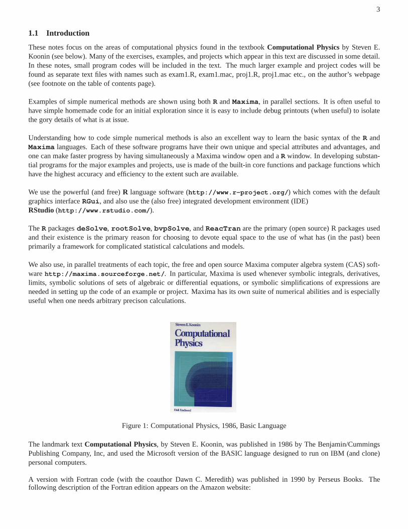
Figure 1: Computational Physics, 1986, Basic Language
The landmark textComputational Physics, by Steven E. Koonin, was published in 1986 by The Benjamin/CummingsPublishing Company, Inc, and used the Microsoft version of the BASIC language designed to run on IBM (and clone)personal computers.
A version with Fortran code (with the coauthor Dawn C. Meredith) was published in 1990 by Perseus Books. Thefollowing description of the Fortran edition appears on theAmazon website:
4
Computational Physics is designed to provide direct experience in the computer modeling of physical systems. Its scopeincludes the essential numerical techniques needed to “do physics” on a computer. Each of these is developed heuris-tically in the text, with the aid of simple mathematical illustrations. However, the real value of the book is in the eightExamples and Projects, where the reader is guided in applying these techniques to substantial problems in classical,quantum, or statistical mechanics. These problems have been chosen to enrich the standard physics curriculum at theadvanced undergraduate or beginning graduate level. The book will also be useful to physicists, engineers, and chemistsinterested in computer modeling and numerical techniques.Although the user-friendly and fully documented programsare written in FORTRAN, a casual familiarity with any other high-level language, such as BASIC, PASCAL, or C,is sufficient. The codes in BASIC and FORTRAN are available onthe web at http://www.computationalphysics.info.They are available in zip format, which can be expanded on UNIX, Window, and Mac systems with the proper soft-ware. The codes are suitable for use (with minor changes) on any machine with a FORTRAN-77 compatible compileror BASIC compiler. The FORTRAN graphics codes are availableas well. However, as they were originally written torun on the VAX, major modifications must be made to make them run on other machines.
Although both of these versions are now out of print, used copies are available via the web (for example at Amazon.com)for as little as ten dollars for the Fortran version and six dollars for the Basic version. The reader of these notes will gainmore understanding of the examples worked out here (using Maxima or the R language) by also reading either of theKoonin texts. For the “Examples” and “Projects”, (and for the average reader) the Basic code will probably be easier tofollow than the Fortran code.
Westview Press, part of the Perseus Books Group, at the address:http://www.westviewpress.com/book.php?isbn=97802013 86233offers the following prices (available in lightening printmode):
Computational Physics Fortran Version, by Steven E. Koonin ,August 1998 Trade Paperback, 656 Pages, $77.00 U.S.,
$88.99 CAN, 51.99 U.K., 54.99 E.U., ISBN 9780201386233
When you click the buy icon on the Westview Press webpaqe, youare offered a list of online book sellers, such as Amazon.com, anda list of local booksellers, such as Barnes and Noble.
The booksamillion.com website athttp://www.booksamillion.com/product/9780201386233# overviewoffers the new paperback for$77 :
The fortran codes and the Basic codes are available as separate zip files athttp://www.computationalphysics.info/ .
From the section “How to use this book” in the Basic version:
This book is organized into chapters, each containing a textsection, an example, and a project. Each text section isa brief discussion of one or several related numerical techniques, often illustrated with simple mathematical examples ...
The example and project in each chapter are applications of the numerical techniques to particular physical problems.Each includes a brief exposition of the physics, followed bya discussion of how the numerical techniques are to beapplied.
The examples and projects differ only in that the student is expected to use (and perhaps modify) the program which isgiven for the former in Appendix B while the book provides guidance in writing programs to treat the latter through aseries of steps...
However, programs for the projects have been included in Appendix C; these can serve as models for the student’sown program or as a means of investigating the physics without having to write a major program “from scratch”. Anumber of suggested studies accompany each example and project; these guide the student in exploiting the programsand understanding the physical principles and numerical techniques involved.
5
The table of contents of Koonin’sComputational Physicsfollows:
Chapter 1: Basic Mathematical Operations1.1 Numerical Differentiation1.2 Numerical Quadrature1.3 Finding Roots1.4 Semiclassical quantization of molecular vibrationsProject I: Scattering by a central potential
Chapter 2: Ordinary Differential Equations2.1 Simple Methods2.2 Multistep and implicit methods2.3 Runge-Kutta methods2.4 Stability2.5 Order and chaos in two-dimensional motionProject II: The structure of white dwarf stars
II.1 The equations of equilibriumII.2 The equation of stateII.3 Scaling the equationsII.4 Solving the equations
Chapter 3: Boundary Value and Eigenvalue Problems3.1 The Numerov algorithm3.2 Direct integration of boundary value problems3.3 Green’s function solution of boundary value problems3.4 Eigenvalues of the wave equation3.5 Stationary solutions of the one-dimensional Schroedin ger equationProject III: Atomic Structure in the Hartree-Fock approxim ation
III.1 Basis of the Hartree-Fock approximationIII.2 The two-electron problemIII.3 Many-electron systemsIII.4 Solving the equations
Chapter 4: Special Functions and Gaussian Quadrature4.1 Special functions4.2 Gaussian quadrature4.3 Born and eikonal approximations to quantum scatteringProject IV: Partial wave solution of quantum scattering
IV.1 Partial wave decomposition of the wavefunctionIV.2 Finding the phase shiftsIV.3 Solving the equations
Chapter 5: Matrix Operations5.1 Matrix inversion5.2 Eigenvalues of a tri-diagonal matrix5.3 Reduction to tri-diagonal form5.4 Determining nuclear charge densitiesProject V: A schematic shell model
V.1 Definition of the modelV.2 The exact eigenstatesV.3 Approximate eigenstatesV.4 Solving the model
Chapter 6: Elliptic Partial Differential Equations6.1 Discretization and the variational principle6.2 An iterative method for boundary-value problems6.3 More on discretization6.4 Elliptic equations in two dimensions
6
Project VI: Steady-state hydrodynamics in two dimensionsVI.1 The equations and their discretizationVI.2 Boundary ConditionsVI.3 Solving the equations
Chapter 7: Parabolic Partial Differential Equations7.1 Naive discretization and instabilities7.2 Implicit schemes and the inversion of tri-diagonal matr ices7.3 Diffusion and boundary value problems in two dimensions7.4 Iterative methods for eigenvalue problems7.5 The time-dependent Schroedinger equationProject VII: Self-organization in chemical reactions
VII.1 Description of the modelVII.2 Linear stability analysisVII.3 Numerical solution of the model
Chapter 8: Monte Carlo Methods8.1 The basic Monte Carlo strategy8.2 Generating random variables with a specified distribut ion8.3 The algorithm of Metropolis et al.8.4 The Ising model in two dimensionsProject VIII: Quantum Monte Carlo for the H2 molecule
VIII.1 Statement of the problemVIII.2 Variational Monte Carlo and the trial wavefunctionVIII.3 Monte Carlo evaluation of the exact energyVIII.4 Solving the problem
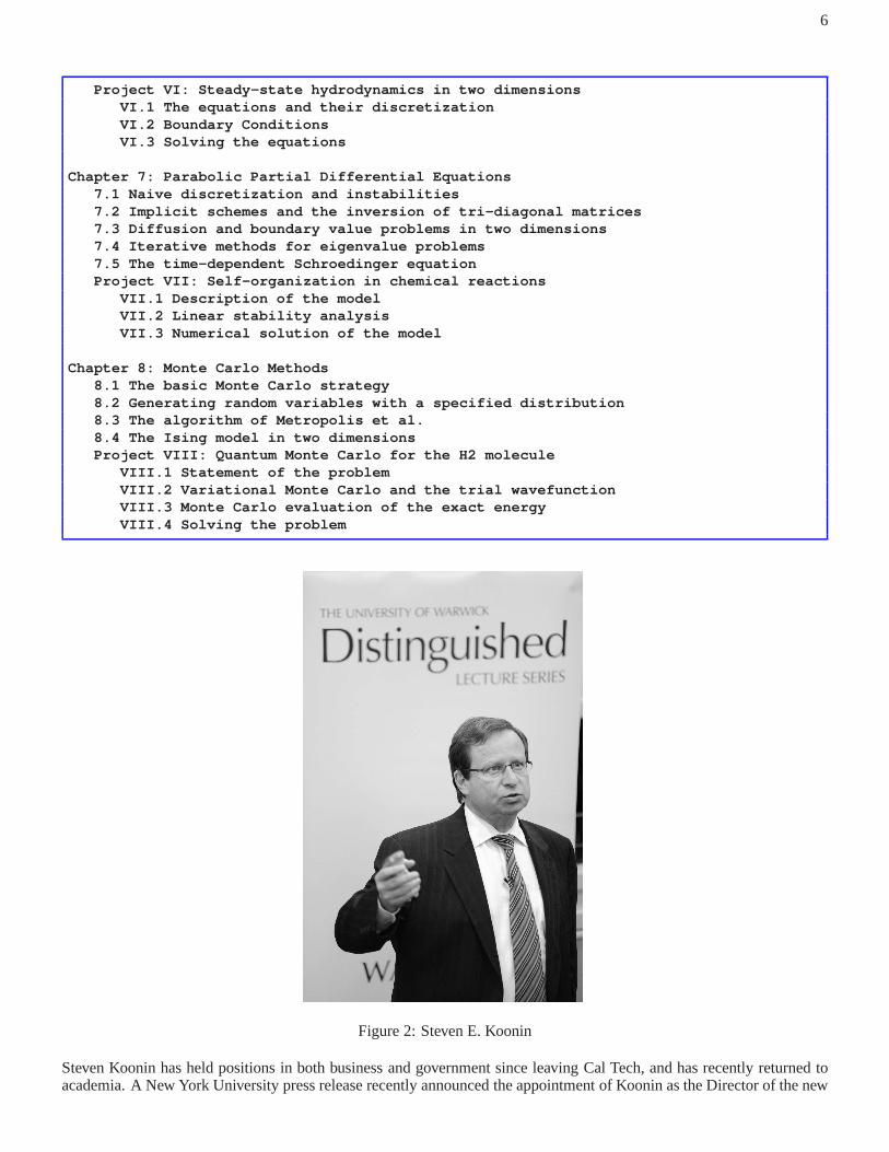
Figure 2: Steven E. Koonin
Steven Koonin has held positions in both business and government since leaving Cal Tech, and has recently returned toacademia. A New York University press release recently announced the appointment of Koonin as the Director of the new
7
Center for Urban Science and Progress (CUSP). Here is a partial quote from that announcement:
Dr. Koonin was confirmed by the Senate in May, 2009 as Undersecretary for Science at the U.S. Department of En-ergy, serving in that position until November, 2011. Prior to joining the Obama Administration, he was BPs ChiefScientist, where he was a strong advocate for research into renewable energies and alternate fuel sources. He came toBP in 2004 following almost 3 decades as Professor of Theoretical Physics at the California Institute of Technology,serving as the Institute’s Vice President and Provost for the last nine years. Koonin comes to CUSP most immediatelyfrom a position at the Science and Technology Policy Institute of the Institute for Defense Analyses in Washington, DC.
Koonin’s research interests have included nuclear astrophysics; theoretical nuclear, computational, and many-bodyphysics; and global environmental science. He has been involved in scientific computing throughout his career. Hehas supervised more than 30 PhD students, produced more than200 peer-reviewed research publications, and authoredor edited 3 books, including a pioneering textbook on Computational Physics in 1985. As Caltech’s Provost, Kooninoversaw its research and educational programs, including the hiring of one-third of the Institute’s faculty. At BP, heconceived and established the Energy Bioscience Instituteat UC Berkeley and the University of Illinois, while at DOE,he led the preparation of both its most recent Strategic Planand its first Quadrennial Technology Review for energy.Koonin has served as an advisor for numerous academic, government, and for-profit organizations.
Dr. Koonin is the recipient of numerous awards and honors, including the George Green Prize for Creative Scholarshipat Caltech, a National Science Foundation Graduate Fellowship, an Alfred P. Sloan Foundation Fellowship, and aSenior U.S. Scientist Award (Humboldt Prize), and the Department of Energy’s Ernest Orlando Lawrence Award. Heis a Fellow of several professional societies, including the American Physical Society, the American Association of theAdvancement of Sciences, and the American Academy of Arts and Sciences, and a member of the Council on ForeignRelations and the U.S. National Academy of Sciences.
A good 3 minute YouTube video of Steven Koonin summarizing his critique of cold fusion at a science conference inBaltimore in 1989 is available athttp://www.youtube.com/watch?v=wR-AohRWbBo . The author enjoyed a similarpresentation by Koonin at the weekly Physics Department Colloquium at California State University at Long Beach inthat same year.
1.2 Choice of R Interfaces and Elements of the R Language
If you are new to theR language, you should first download and install the latest (free and open source) Windows versionof R from http://www.r-project.org/ , choosing the default answers for all questions asked during the install pro-cess. You should see theR icon on your desktop. Clicking that icon will start up the default user interface, a Windows IDEcalledRGui , with a blinking cursor in theR Console window. This interface will allow you to start getting familiarwith theR language.
You can customize the look of the Console window using the menu barEdit, GUIpreferences... ,
The author’s settings are 1. checked boxes: MDI, MDI Toolbar, multiple windows, and True Type only, 2. Font set toCourier New, Font size set to 12, Font style set to bold, 3. Console rows = 25, Console columns = 80, 4. backgroundcolor = wheat1, normal text color = black, user text color = blue, pagerbg color = white.
Keyboard Shortcuts
SelectHelp, Console to get a window of keyboard shortcuts. One of the most useful is the two key commandCtrl+Tab to toggle between the Console window and the graphics window(“device”). Another keyboard shortcutto get back to the Console window (from a graphics window, forexample,) is(Alt+w, 1) , which makes use of theWindows submenu.
To clear the screen and move the cursor to the top of the Console window, use the keyboard shortcutCtrl+l (lowercaseof letter L), or else use(Edit, Clear console) .The up-arrow and down-arrow keys cycle through the “commandhistory”. The up-arrow key of the keyboard only bringsin one line at a time from the previous inputs, which is not convenient to bring into action a multiline input. It is alsovery difficult to edit a multiline command inside theRGui Console window. Hence the author recommends that multiline
8
input commands be set up in a text editor (containing a daily “work diary”, for example) such as Notepad2 or Notepad++which have strong parenthesis and bracket matching features, and be pasted into the Console (usingCtrl+v ) to try outthe current code. You can set up multiple function definitions and parameter assignments, copy the whole group to theclipboard (usingCtrl+c ), and then paste the whole group into the console at once using Ctrl+v .
Getting work done in the Console window is a little primitive. The INS key toggles the overwrite mode on and off (ini-tially off). When editing a line in the Console, you can use the Home, End, left-arrow , andright-arrow keys tomove left and right. You can use either thebackspace and/or thedelete keys to delete characters. Youcannot useShift+right-arrow to highlight a set of contiguous characters. Youcannot useShift+End to highlight part or all ofa line. However,Ctrl+Del will delete from the current character to the end of the current line, andCtrl+U will deleteall text from the current line.
Clicking on the Console window does not move the cursor.Ctrl+Home and Ctrl+End do nothing. Page-Up andPage-Down do nothing. To copy only some lines of input and output for transfer back to your text based work file orto a LaTeX document, you must drag the cursor over the lines desired to highlight, and then useCtrl+c to copy to theclipboard.
You can copyall the current Console windows contents (i.e., since the last use ofCtrl+l ) using(Edit, Select All) ,and then either(Edit, Copy) or Ctrl+C . To turn off the selection highlight, you can either press the Backspace keyor use the mouse to click in the Console window.
Use repeated down-arrow’s to restore the cursor to the interpreter prompt. Pressing theEsc key will also restore theinterpreter prompt (and will also stop the interpreters current action).
Entering, for example,?curve will launch a full page browser view of documentation for theR functioncurve , a viewmode which is easier to read and copy from compared with the rather constricted help panel in the RStudio environment(see below). Entering justcurve without the leading question mark, and without any(...) will display theR codewhich defines the function.
To quit R, useq() , (followed as usual byEnter ). You will be asked if you want to save the current state of thework andsettings, which requires pressing either the lettern or y .
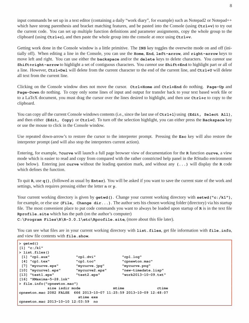
Your current working directory is given bygetwd() . Change your current working directory withsetwd("c:/k1") ,for example, or else use(File, Change dir...) . The author sets his chosen working folder (directory) via his startupfile. The most convenient place to put code commands you want to always be loaded upon startup ofR is in the text fileRprofile.site which has the path (on the author’s computer)C:\Program Files\R\R-3.0.1\etc\Rprofile.site , (more about this file later).
You can see what files are in your current working directory with list.files , get file information withfile.info ,and view file contents withfile.show .
The last command (file.show ) opened up a separate window called the R Information window, where the contents ofthe file were displayed.
Thecat function in theRGui Console does not automatically add a “line advance” in interactive use (as doesRStudio ).Instead you need to add a string"\n" as the last element:
> a=2; b = 4; c = 6> cat(a,b,c)2 4 6> cat(a,b,c,"\n")2 4 6
Depending on your aptitude for dealing with a busy environment, you might wish to download (fromhttp://www.rstudio.org/ the (free and open source)RStudio integrated development environment (IDE), which makes it easierto keep track of what objects are currently known in the workspace, which packages are currently loaded, and has easilyseen windows for help documentation requested, plots made,a window of a history of commands used in interactive use,and a window displaying the files in the current folder. And the submenu brought up via the Session menu choice makesit easy to set the “working directory” (working folder). There is also a text window (called Source) for writing and editingcode which has an easy method for pasting into the Console window.
The Console window of RStudio is the place to either type in orpaste in (from either the Source window or from a texteditor such as the free and very usefulNotepad2 (http://sourceforge.net/projects/notepad2/ ). PressingEnter at the end of such Console input will causeR to interpret and “run” the command(s).
You can enlarge the width of the Console window by dragging onthe right hand border of the Console window. However,if you try to expand the width of the Console window too far, the present behavior suddenly pushes the normal right win-dow panes out of sight, and you must do some serious dragging from the right edge to recover the normal multiple paneview; there is apparently no keyboard command which will restore the default view and size of theRStudio windows.
To return the cursor to the Console window, when in any other RStudio window, use the two-key commandCtrl+2 .There are fast keyboard shortcuts for most things. To clear the Console screen and place the cursor at the top of the Con-sole window, useCtrl+l (that is lower case letterl , not number1). To quitR, useq() , (followed as usual byEnter ).
If you happen to choose (from the munu)(File, Close All) , the Source window will vanish. You can restore analtered version using either:(File, New, Rscript) , or File, New, Text File , or File, Open ... . Then youcan return the cursor to the Source window usingCtrl+1 (number1).
You should then go to theRStudio documentation pagehttp://www.rstudio.com/ide/docs/ and work throughthe nine sections of tutorial material under the headingUsing RStudio , with the following sections: Working in theConsole, Editing and Executing Code, Code Folding and Sections, Navigating Code, Using Projects, Command History,Working Directories and Workspaces, Customizing RStudio,Keyboard Shortcuts. The sections on Code Folding, Projectsand Customizing are of very secondary interest to a new user.
A somewhat controversial subject is whether one should restrict oneself to the notation<- for “assignment” inR, or whether it iskosher to use instead the equal sign= in place of<- . Thusa <- 3.2 or myf <- function(x,y) {x * sin(y)} are respec-tively an assignment of the floating point number3.2 to the symbola, and the assignment of a function definition to the symbolmyf , the latter used with the syntaxb <- myf(2,1.2) , for example.
Either<- or = will result in correctly behaving code in practice. Puristsin Rdenigrate the use of the equal sign= for the assignmentoperation. Physicists are used to choosing the easiest method of getting the job done. The author prefers the equal sign for assignmentbecause it requires one keyboard operation, rather than two, and also because the resulting code can be more speedily visuallyscanned. The<- notation slows the visual scan speed, because one needs to besure a minus sign was not inadvertently inserted at aposition not intended. Thus the author usesa = 3.2 andmyf = function(x,y) {x * sin(y)} .
10
Miscellaneous Tips on R
R treats the symbolsn andNas distinct. (Case matters.)
The author prefers to expand theConsole window (of RStudio ) both vertically and horizontally (the latter by drag-ging the window edge, but not too large!). When you then make aplot, the plot window will become automaticallyvisible, but will be small. You can either drag the edge of theplot window to the left, to see more clearly, and/or youcan click on the zoom icon near the top of the plot window, thuscreating a much larger and dedicated window for the plot.
The author prefers to design code in a text editor such asNotepad2(see above mention) partly because the editor usesstrong color contrast for matching parentheses and brackets, and it is easy to see if you have missed some closing paren-theses or brackets. You can select one or moreR statements and paste them into theConsole as long as the end of eachline of code in clearly incomplete or clearly complete. If a line of code in the text editor needs completion on the nextline, split the line after a comma, for example so that theR interpreter knows more must be coming.
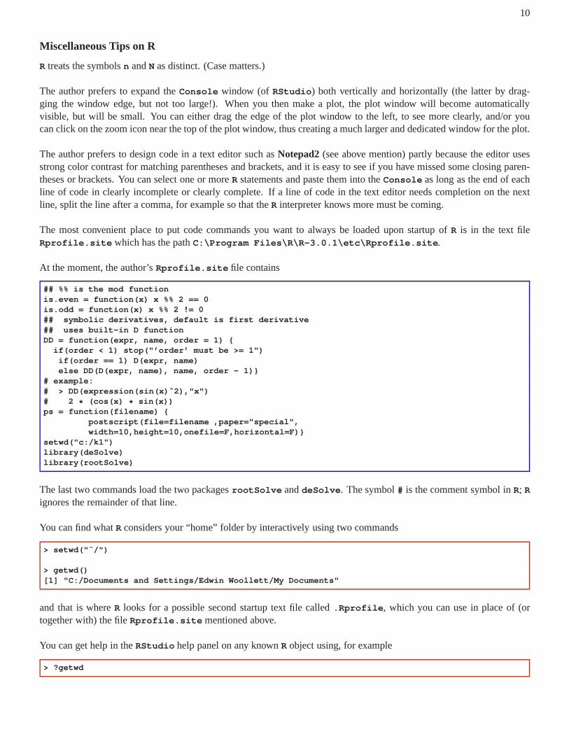
The most convenient place to put code commands you want to always be loaded upon startup ofR is in the text fileRprofile.site which has the pathC:\Program Files\R\R-3.0.1\etc\Rprofile.site .
At the moment, the author’sRprofile.site file contains
## %% is the mod functionis.even = function(x) x %% 2 == 0is.odd = function(x) x %% 2 != 0## symbolic derivatives, default is first derivative## uses built-in D functionDD = function(expr, name, order = 1) {
if(order < 1) stop("’order’ must be >= 1")if(order == 1) D(expr, name)else DD(D(expr, name), name, order - 1)}
The last two commands load the two packagesrootSolve anddeSolve . The symbol# is the comment symbol inR; R
ignores the remainder of that line.
You can find whatR considers your “home” folder by interactively using two commands
> setwd("˜/")
> getwd()[1] "C:/Documents and Settings/Edwin Woollett/My Documen ts"
and that is whereR looks for a possible second startup text file called.Rprofile , which you can use in place of (ortogether with) the fileRprofile.site mentioned above.
You can get help in theRStudio help panel on any knownR object using, for example
> ?getwd
11
and theRStudio help panel will display the documentation.
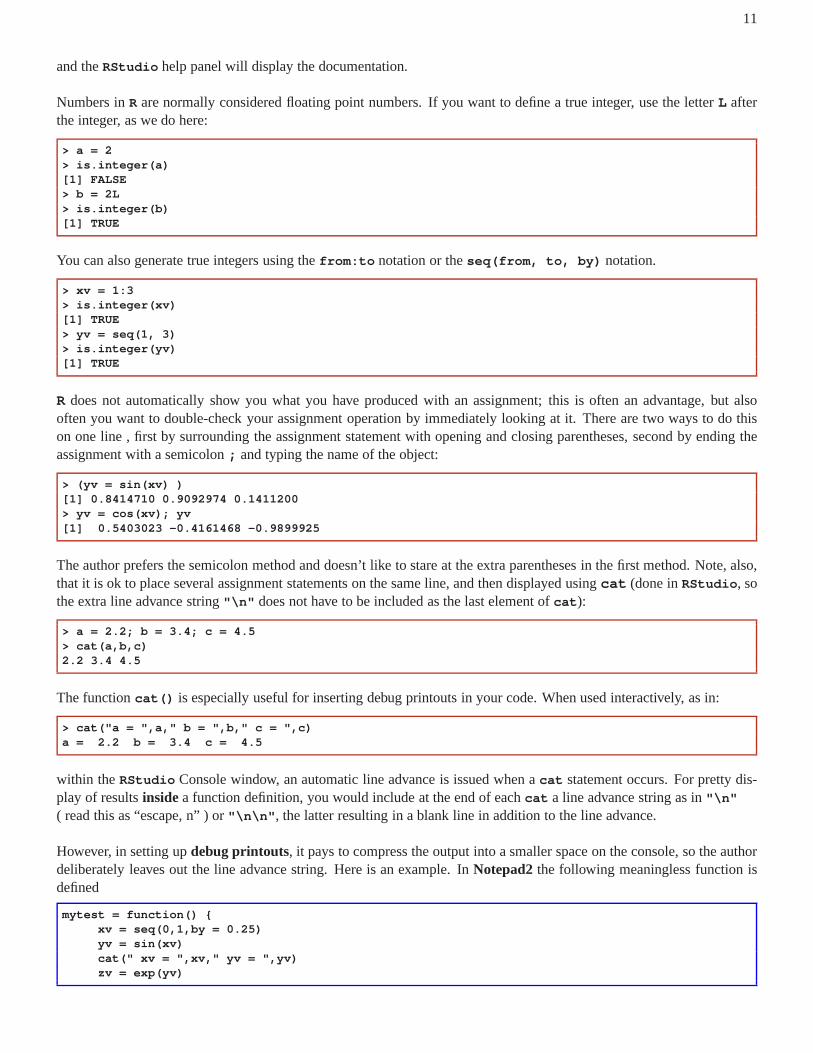
Numbers inR are normally considered floating point numbers. If you want to define a true integer, use the letterL afterthe integer, as we do here:
> a = 2> is.integer(a)[1] FALSE> b = 2L> is.integer(b)[1] TRUE
You can also generate true integers using thefrom:to notation or theseq(from, to, by) notation.
R does not automatically show you what you have produced with an assignment; this is often an advantage, but alsooften you want to double-check your assignment operation byimmediately looking at it. There are two ways to do thison one line , first by surrounding the assignment statement with opening and closing parentheses, second by ending theassignment with a semicolon; and typing the name of the object:
The author prefers the semicolon method and doesn’t like to stare at the extra parentheses in the first method. Note, also,that it is ok to place several assignment statements on the same line, and then displayed usingcat (done inRStudio , sothe extra line advance string"\n" does not have to be included as the last element ofcat ):
> a = 2.2; b = 3.4; c = 4.5> cat(a,b,c)2.2 3.4 4.5
The functioncat() is especially useful for inserting debug printouts in your code. When used interactively, as in:
> cat("a = ",a," b = ",b," c = ",c)a = 2.2 b = 3.4 c = 4.5
within theRStudio Console window, an automatic line advance is issued when acat statement occurs. For pretty dis-play of resultsinsidea function definition, you would include at the end of eachcat a line advance string as in"\n"
( read this as “escape, n” ) or"\n\n" , the latter resulting in a blank line in addition to the line advance.
However, in setting updebug printouts, it pays to compress the output into a smaller space on the console, so the authordeliberately leaves out the line advance string. Here is an example. InNotepad2the following meaningless function isdefined
as a demonstration of what happens when you leave out the lineadvance string at the end of all but the lastcat . Theabove code was selected and copied to the Windows Clipboard,and then pasted into theRStudio console, and then thefunction was tried out.R adds a+ sign to the beginning of each successive line, indicating itknows the code fragment isnot yet complete (since the final closing bracket has not yet been found).
(If you try this in the defaultRGui interface, the output is on one very long line, so you must scroll the screen rightwardto see everything, and the visible portion ends with a$ to warn you there is more. But if you drag and copy the screen,you get the whole output.)
With both interfaces, if you copy the screen and paste into averbatim section of a LaTeX file, after running LaTeX,thedvi file will show only part of the long line; you must line break manually in the LaTeX file.
R, by default, displays 7 digits for floating point numbers (while internally using 16 digit arithmetic). To make thecompressed debug output even more convenient, we can use theoptions(digits = m) command, and re-run thefunction:
R has no single precision data type. All real floating point numbers are stored in double precision format. Hence thecoercive functionsas.numeric() , as.double() , andas.single() all do the same job.
A vector inR is not necessarily a physical vector, but is an ordered collection of objects of the same type.xv = 1:10
definesxv as a vector, and so doesxv = seq(1,10) , and so doesxv = c(1,2,3,4,5,6,7,8,9,10) . The c()
function is one of the most usedR functions, and the ‘c’ stands for ‘concatenate’. Individual elements of a vectorxv areaccessed using a single bracket, as inxv[3] .
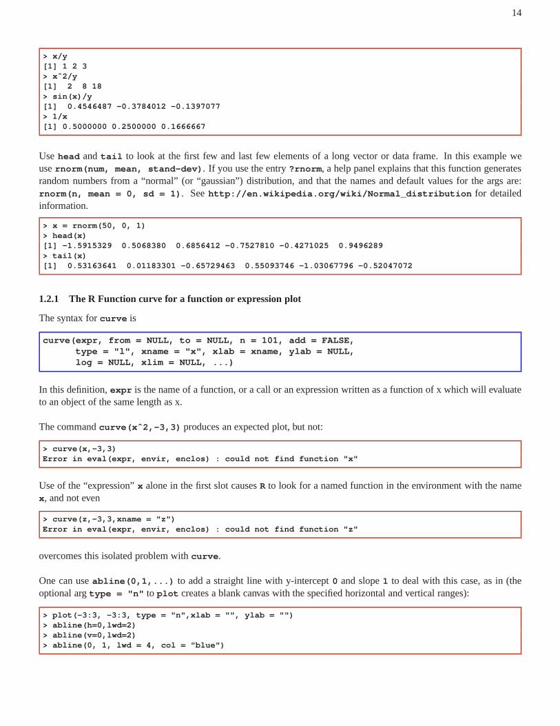
Usehead and tail to look at the first few and last few elements of a long vector ordata frame. In this example weusernorm(num, mean, stand-dev) . If you use the entry?rnorm , a help panel explains that this function generatesrandom numbers from a “normal” (or “gaussian”) distribution, and that the names and default values for the args are:rnorm(n, mean = 0, sd = 1) . Seehttp://en.wikipedia.org/wiki/Normal_distribution for detailedinformation.
1.2.1 The R Function curve for a function or expression plot
The syntax forcurve is
curve(expr, from = NULL, to = NULL, n = 101, add = FALSE,type = "l", xname = "x", xlab = xname, ylab = NULL,log = NULL, xlim = NULL, ...)
In this definition,expr is the name of a function, or a call or an expression written asa function of x which will evaluateto an object of the same length as x.
The commandcurve(xˆ2,-3,3) produces an expected plot, but not:
> curve(x,-3,3)Error in eval(expr, envir, enclos) : could not find function "x"
Use of the “expression”x alone in the first slot causesR to look for a named function in the environment with the namex , and not even
> curve(z,-3,3,xname = "z")Error in eval(expr, envir, enclos) : could not find function "z"
overcomes this isolated problem withcurve .
One can useabline(0,1,...) to add a straight line with y-intercept0 and slope1 to deal with this case, as in (theoptional argtype = "n" to plot creates a blank canvas with the specified horizontal and vertical ranges):
but beware: inplot(x,y,...) the vectorsx andy must be thesame length.
Use of eithercurve(xˆ2 - 5, -3, 3) or curve(yˆ2 - 5,-3,3,xname = "y") will draw the same figure. Thevalue ofxname defaults to"x" .
You can increase the number of function samples taken for theplot by overriding the default value ofn, for exam-ple with curve(xˆ2-5,-3,3,200) , or by using named arguments, avoiding respecting the orderof the arguments:curve(xˆ2-5,-3,3,lwd=3,col = "blue",n = 200) .
The lwd parameter defaults tolwd = 1 , so usinglwd=3 makes the line three times as thick. The default line type forcurve is a solid line (lty = 1 ), and the default color iscol = "black" .
TheR functionsplot , matplot , points , abline , andlines can each deal with additional args involvinglty , lwd ,col , andtype .
To avoid the default labels on the horizontal (“x”) axis and the vertical (“y”) axis, you can includexlab = "" andylab = "" , or else furnish your own string, such asxlab = "time (sec)" .
The default behavior ofcurve (add = FALSE) starts a new figure, ignoring any past graphics commands. If you want toadd additional elements to your initial plot, the “high-level” function (such ascurve or plot ) needs to be invoked withthe extra argadd = TRUE. In contrast, using any of the “low-level” functionspoints , or abline or lines simply addsto your initial plot.
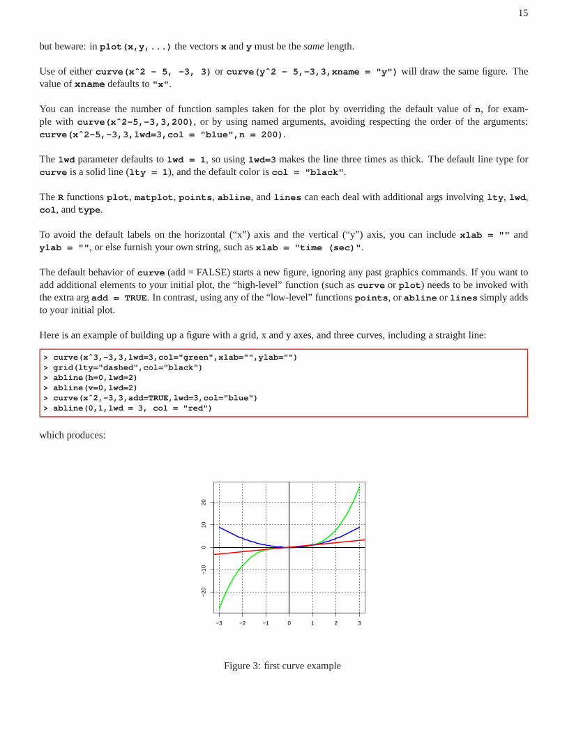
Here is an example of building up a figure with a grid, x and y axes, and three curves, including a straight line:
A long list of contributed documents onRwhich are available on the web can be found athttp://cran.r-project.org/other-docs.html
and links to document collections, Journals, and Proceedings can be found athttp://www.r-project.org/other-docs.html
A very useful 103 page tutor in both a pdf and html version is found with your local installation ofR. On the author’scomputer it is located atC:\Program Files\R\R-3.0.1\doc\manual\R-intro.pdf
andC:\Program Files\R\R-3.0.1\doc\manual\R-intro.html , and is titled“An Introduction to R: Notes onR: A Programming Environment for Data Analysis and Graphics” , by W.N. Venables, D.M. Smith, and the R CoreTeam.
Whether or not you have some prior knowledge ofMatlab , you will find a very well organized 52 page pdf comparisonof Matlab andR syntax, organized by the type of operation desired, athttp://www.math.umaine.edu/˜hiebeler/comp/matlabR.h tml .
An 83 page pdf introduction toR by active scientific researchers including the co-author of“Solving Differential Equa-tions in R” is a pdf document titled“Using R for Scientific Computing” by Karline Soetaert and Filip Meysman(2011),which can be found athttp://vkc.library.uu.nl/vkc/darwin/knowledgeportal /Lists/
Conferences/Attachments/28/Meysman_ScienceR.pdf
18
and an earlier 46 page version dated 2008 with the single author Karline Soetaert:http://cran.r-project.org/doc/contrib/Soetaert_Scie ntificcomputing.zip , which, when unzipped,
contains ScientificComputing.pdf with document title “Using R for Scientific Computing”.
The 2009 46 page version can be found athttps://r-forge.r-project.org/scm/viewvc.php/pkg/ma relacTeaching/inst/
doc/lecture/?root=marelac&sortby=rev&pathrev=122
1.3 Elements of the Maxima Language
Users new to Maxima should work through some of the tutorialswhich can be found under the Documentation tab on theMaxima CAS project page:http://maxima.sourceforge.net/ Chapters 1 - 3 of the author’sMaxima by Example would be sufficient.
The author always uses thexmaxima.exe interface, located in...\bin . A useful keyboard feature of Xmaxima is theuse of the two-key commandAlt+p . Used once, or multiple times, you can easily repeat a previous command, but youfirst have the opportunity to edit it before pressing Enter.
The usual keyboard commands allow easy movement within the Xmaxima window:Home(beginning of line),End (endof line), PageUp, PageDown, UpArrow , DownArrow , Ctrl+Home (top of window),Ctrl+End (bottom of window).
See the discussion of how to arrange your work folder and the startup options in ch.1 of the author’s set of notes:Maxima by Example . Google ’ted woollett’ and those notes will be at the first hit. The author uses the startup fileto send the commanddisplay2d:false to Maxima for routine use. This allows more information to bein the Xmax-ima window at a time, and allows for easier selection and copying of portions of the work for transfer to a work text fileor the verbatim section of a tex file. The code fragments copied into verbatim sections of a tex file also then take up lessroom when converted to a pdf file.
Case matters in Maxima.
(%i1) a : 2;(%o1) 2(%i2) A : 3;(%o2) 3(%i3) [a, A];(%o3) [2,3](%i4) if a = A then print("equal") else print("not equal")$not equal
Learn the crucial difference between usingmapandapply with a Maxima list. Supposef is some core or homemadefunction (here the definition off is unknown to Maxima):
mod is the Maxima modulus function. A useful example ofapply is with the"+" function:
(%i10) apply("+",[2,4,6,8]);(%o10) 20
19
which adds up the elements in the given list. If you have a named list, the “apply” method is faster than using the coreMaxima functionsum:
(%i11) xv : makelist(i,i,1,10);(%o11) [1,2,3,4,5,6,7,8,9,10](%i12) apply("+",xv);(%o12) 55(%i13) sum(xv[i],i,1,length(xv));(%o13) 55
Many core Maxima functions (such asfloat ) automatically distribute over lists, so the use ofmap is not always requiredto get the job done. The Lisp code which defines the core function determines whether or not that function distributesover lists. Let’s check the functionsin :
(%i14) sin([1,2]);(%o14) [sin(1),sin(2)](%i15) properties(sin);(%o15) ["mirror symmetry",deftaylor,integral,"distrib utes over bags",rule,
noun,gradef,transfun]
The Maxima functionproperties can be used with core functions and the element"distributes over bags"
indicates thatsin distributes over lists (provided a global parameterdistribute_over is set totrue (the default)).See the Maxima help manual (in XMaxima, select the menu item:Help, Maxima Manual), and using theindex mode,type in the start ofdistributes_over and select help by pressing Enter. The result starts out:
distribute_over controls the mapping of functions over bag slike lists, matrices, and equations. At this time not allMaxima functions have this property. It is possible tolook up this property with the command properties.
The mapping of functions is switched off, when settingdistribute_over to the value false.
Examples:
The sin function maps over a list:
(%i1) sin([x,1,1.0]);(%o1) [sin(x), sin(1), .8414709848078965]mod is a function with two arguments which maps over lists.
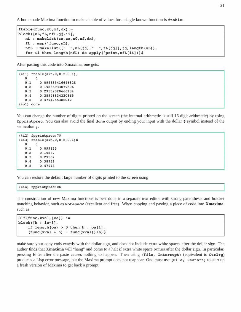
You can change the number of digits printed on the screen (theinternal arithmetic is still 16 digit arithmetic) by usingfpprintprec . You can also avoid the finaldone output by ending your input with the dollar$ symbol instead of thesemicolon; .
You can restore the default large number of digits printed tothe screen using
(%i4) fpprintprec:0$
The construction of new Maxima functions is best done in a separate text editor with strong parenthesis and bracketmatching behavior, such asNotepad2 (excellent and free). When copying and pasting a piece of code intoXmaxima,such as
D1f(func,xval,[oa]) :=block([h : 1e-8],
if length(oa) > 0 then h : oa[1],(func(xval + h) - func(xval))/h)$
make sure your copy ends exactly with the dollar sign, and does not include extra white spaces after the dollar sign. Theauthor finds thatXmaxima will “hang” and come to a halt if extra white space occurs after the dollar sign. In particular,pressing Enter after the paste causes nothing to happen. Then using (File, Interrupt) (equivalent toCtrl+g )produces a Lisp error message, but the Maxima prompt does notreappear. One must use(File, Restart) to start upa fresh version of Maxima to get back a prompt.
22
1.3.1 The Maxima Function plot2d
The first curve example done usingRcan be done with oneplot2d command using Maxima. If we use the default colorcycle of Maxima, as in
the default color scheme results in the first (cubic) function drawn in blue, the second (quadratic) function drawn in red,and the third (linear) function drawn in green.
To get the same color choices in our firstR example, we need a more involvedplot2d command, which forces colorchoices for each of the three functions in the list:
The line syntax is[lines, width, color] , with the default line width being1, and the color choices being: 1:blue,2:red, 3: green, 4: violet, 5: brown, 6:black, 7:blue, . . . .
To get the same color choices in our secondRexample, we can use
Much more information about Maxima’splot2d function can be found in Chapter 2 ofMaxima by Example on theauthor’s webpage.
1.4 Numerical Derivatives
Seehttp://en.wikipedia.org/wiki/Numerical_derivative for a discussion of different types of numericalderivative approximations.
In Computational Physics, ch 1, Sec.1, Koonin uses Taylor series expansions to derive what he calls a “3 point” approxi-mation to the first derivative of a functionf at some pointx
The second and third terms on the right hand side (the error terms) are zero if the third and higher derivatives of the givenfunction vanish at the positionx , which would be the case if the function is an arbitrary second degree polynomial in theinterval [x-h, x+h] . (All the error terms in the above involve even powers ofh.) If the function’s third derivative isnot zero, the error terms can in principle be made arbitrarily small by lettingh shrink to zero. However arithmetic inRis done with only 16 digit accuracy, and this means there is a limit to how small we can takeh in practice, related to theprocess of finding the difference of two almost equal floatingpoint numbers and in the process losing significant digits ofprecision (roundoff error).
We will call the following a “central difference” approximation to the numerical derivative off atx
f’(x) = ( f(x+h) - f(x-h) )/(2 * h) + O(hˆ2)
23
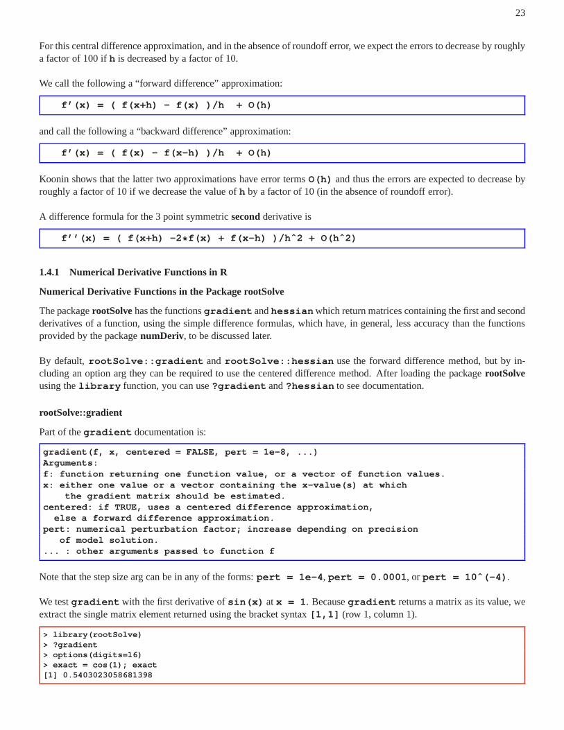
For this central difference approximation, and in the absence of roundoff error, we expect the errors to decrease by roughlya factor of 100 ifh is decreased by a factor of 10.
We call the following a “forward difference” approximation:
f’(x) = ( f(x+h) - f(x) )/h + O(h)
and call the following a “backward difference” approximation:
f’(x) = ( f(x) - f(x-h) )/h + O(h)
Koonin shows that the latter two approximations have error termsO(h) and thus the errors are expected to decrease byroughly a factor of 10 if we decrease the value ofh by a factor of 10 (in the absence of roundoff error).
A difference formula for the 3 point symmetricsecondderivative is
Numerical Derivative Functions in the Package rootSolve
The packagerootSolvehas the functionsgradient andhessian which return matrices containing the first and secondderivatives of a function, using the simple difference formulas, which have, in general, less accuracy than the functionsprovided by the packagenumDeriv, to be discussed later.
By default, rootSolve::gradient and rootSolve::hessian use the forward difference method, but by in-cluding an option arg they can be required to use the centereddifference method. After loading the packagerootSolveusing thelibrary function, you can use?gradient and?hessian to see documentation.
rootSolve::gradient
Part of thegradient documentation is:
gradient(f, x, centered = FALSE, pert = 1e-8, ...)Arguments:f: function returning one function value, or a vector of func tion values.x: either one value or a vector containing the x-value(s) at w hich
the gradient matrix should be estimated.centered: if TRUE, uses a centered difference approximatio n,
else a forward difference approximation.pert: numerical perturbation factor; increase depending o n precision
of model solution.... : other arguments passed to function f
Note that the step size arg can be in any of the forms:pert = 1e-4 , pert = 0.0001 , or pert = 10ˆ(-4) .
We testgradient with the first derivative ofsin(x) atx = 1 . Becausegradient returns a matrix as its value, weextract the single matrix element returned using the bracket syntax[1,1] (row 1, column 1).
We see that the step size1e-6 (smaller than the default), when used with the centered method, leads to much higheraccuracy.
Let’s make a table, usingdata.frame , of fractional errors which compares the forward with the centered method forvarious values ofh. The vector ofh values (the step size) and the fractional error calculations make use ofR’s vectorarithmetic abilities.
> options(digits=3)> hv = 4:10 ; hv[1] 4 5 6 7 8 9 10> numd = vector(mode="numeric",length=length(hv))> for (i in 1:length(hv)){+ numd[i] = gradient(sin,1,pert = 10ˆ(-hv[i]))[1,1]}> numd.c = vector(mode="numeric",length=length(hv))> for (i in 1:length(hv)){+ numd.c[i] = gradient(sin,1,pert = 10ˆ(-hv[i]), centered =TRUE)[1,1]}> data.frame( h = 10ˆ(-hv), forward = (exact - numd)/exact ,+ centered = (exact - numd.c)/exact )
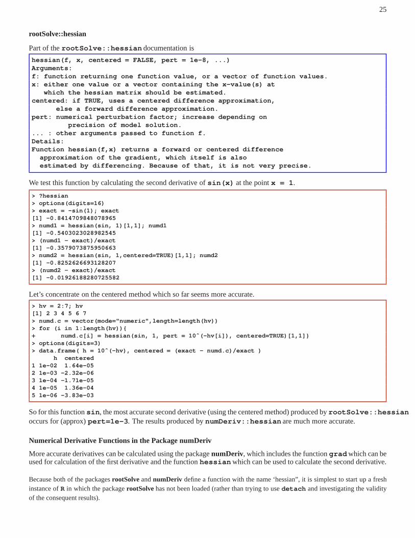
hessian(f, x, centered = FALSE, pert = 1e-8, ...)Arguments:f: function returning one function value, or a vector of func tion values.x: either one value or a vector containing the x-value(s) at
which the hessian matrix should be estimated.centered: if TRUE, uses a centered difference approximatio n,
else a forward difference approximation.pert: numerical perturbation factor; increase depending o n
precision of model solution.... : other arguments passed to function f.Details:Function hessian(f,x) returns a forward or centered differ ence
approximation of the gradient, which itself is alsoestimated by differencing. Because of that, it is not very pr ecise.
We test this function by calculating the second derivative of sin(x) at the pointx = 1 .
So for this functionsin , the most accurate second derivative (using the centered method) produced byrootSolve::hessianoccurs for (approx)pert=1e-3 . The results produced bynumDeriv::hessian are much more accurate.
Numerical Derivative Functions in the Package numDeriv
More accurate derivatives can be calculated using the packagenumDeriv, which includes the functiongrad which can beused for calculation of the first derivative and the functionhessian which can be used to calculate the second derivative.
Because both of the packagesrootSolveandnumDeriv define a function with the name ‘hessian”, it is simplest to start up a freshinstance ofR in which the packagerootSolvehas not been loaded (rather than trying to usedetach and investigating the validityof the consequent results).
26
numDeriv::grad
Part of the documentation produced by using?grad after loading thenumDeriv package usinglibrary is:
grad(func, x, method="Richardson", method.args=list(), ...)Arguments:func: a function with a scalar real result (see details).x: a real scalar or vector argument to func, indicating the
point(s) at which the gradient is to be calculated.method: one of "Richardson", "simple", or "complex" indica ting
the method to use for the approximation.method.args: arguments passed to method. Arguments not spe cified
remain with their default values as specified in details... : additional arguments passed to func. WARNING: None of
these should have names matching other arguments of this fun ction.Value: A real scalar or vector of the approximated gradient( s).
We usegrad to calculate the first derivative ofsin(x) at the pointx = 1. For our example,grad returns a number (nota matrix).
The default method is"Richardson" , which uses Richardson extrapolation (see the?grad help documentation fordetails and references). The"complex" method assumes the given function is analytic in a neighborhood of the evalu-ation pointx .
numDeriv::hessian
Part of the documentation forhessian is
hessian(func, x, method="Richardson", method.args=list (), ...)Arguments:func: a function for which the first (vector) argument is use d as a parameter vector.x: the parameter vector first argument to func.method: one of "Richardson" or "complex" indicating the met hod to
use for the approximation.method.args: arguments passed to method. See grad.
(Arguments not specified remain with their default values. )... : an additional arguments passed to func. WARNING: None o f
these should have names matching other arguments of this fun ction.Value: An n by n matrix of the Hessian of the function calculat ed
at the point x.
27
We usenumDeriv::hessian to calculate the second derivative ofsin(x) at the pointx = 1. We need to extract thesingle matrix element returned for our example using[1,1] (row 1, column 1).
The"simple" method is not supported bynumDeriv::hessian .
1.4.2 Testing Simple Numerical Derivative Methods in R
To test the symmetric centered difference method of finding an approximate numerical derivative, Koonin presents ashort interactive program in which the user provides a valueof step sizeh and the central difference approximation tothe first derivative ofsin(x) is computed atx = 1 , together with the error. The “exact” answer iscos(1) . Thedefault number of digits displayed inR is 7, which can be changed by the user viaoptions(digits = n) . (Useoptions() to see all current options settings, but beware because there are many options.)
in which sprintf allows the use of a formatting string as in theC language.
In order to make a table comparing the errors in evaluating the first derivative ofsin(x) at the pointx = 1 , we definethe functionsD1c, D1f , andD1b which employ the central, forward, and backward differenceformulas, respectively.
D1c = function (func, x, h = 1e-8) {(func(x + h) - func(x - h))/(2 * h) }
In the last entry, instead of a single value ofh, we have used a vector ofh values, in the formc(h1,h2) and obtained theerror for two cases using only one line.
Using this approach we now construct a table of errors (with headings), using the central, forward, and backward differ-ence methods, in computing the first derivative ofsin(x) atx = 1 .
We see that the error of the derivative approximations cannot be made arbitrarily small by continuing to decrease the sizeof h, due the the appearance of roundoff errors made in subtracting two almost equal numbers from each other using 16digit arithmetic.TheR functiondiff is very efficient in taking numerical differences. The differenceb - a = diff(c(a, b)) .
> diff(c(3.1, 4.2))[1] 1.1
We can improveD1c, for example, by employing thediff() function, but the resulting function will not work in thesame way (as above) if the parameterh is set equal to a vector. Here we usediff to explore the roundoff error whenusing the central difference formula withh = 1e-14 .
For this small value ofh the numerical derivative is returned with only two digits ofaccuracy.
1.4.3 Testing Simple Numerical Derivative Methods in Maxima
In Computational Physics, ch 1, Sec.1, Koonin has a short interactive program in which the user provides a value ofhand the central difference approximation to the first derivative of sin(x) is computed atx = 1 , together with the error.The symbolic answer iscos(1) , which is, to 16 digit accuracy,
(%i1) float(cos(1));(%o1) 0.54030230586814
In this section on simple numerical derivatives in Maxima, we will not be as careful with error calculations as we will bein other sections. A more careful approach would be to define an “exact” value, good to 20 digits using bigfloat methods,as in
and then compare a resultval , calculated with some other method using 16 digit arithmetic, with the “exact value” via
block([fpprec:20], bfloat(val - exact))
for “absolute error”, or
block([fpprec:20], bfloat( (val - exact)/exact))
for “fractional error”.
If we translate theRversion oftryh() (above) into Maxima, we must end each command with a comma, wemust use:for assignment instead of=, we must replace curly brackets with parentheses, we must use read or readonly insteadof readline , we must usedo instead ofrepeat to get an endless loop, we must usereturn instead ofbreakto get out of the loop, we must useprint instead ofcat , the if syntax for Maxima requires athen , we can addnumer:true to ensure trig functions are converted to floating point numbers (or else wrap the output infloat ), and,finally, we should avoid the Maxima reserved worddiff (used for symbolic differentiation in Maxima) in our code.
The difference between the Maxima functionsread andreadonly is thatread evaluates the input andreadonlydoes not evaluate the input.
exact : cos(x),print(" enter h <= 0 to stop "),do (
h : read(" input h: "),if h <= 0 then return(done),fprime : 0.5 * (sin(x+h) - sin(x-h))/h,fp_diff : exact - fprime,print(" h = ",h," error = ",fp_diff )))$
After pasting this definition oftryh() into Maxima, we get
(%i3) fpprintprec:4$(%i4) tryh();
enter h <= 0 to stopinput h:
1/20;h = 0.05 error = 2.251E-4input h:
1/40;h = 0.025 error = 5.628E-5input h:
1e-3;h = 0.001 error = 9.005E-8input h:
-1;(%o4) done
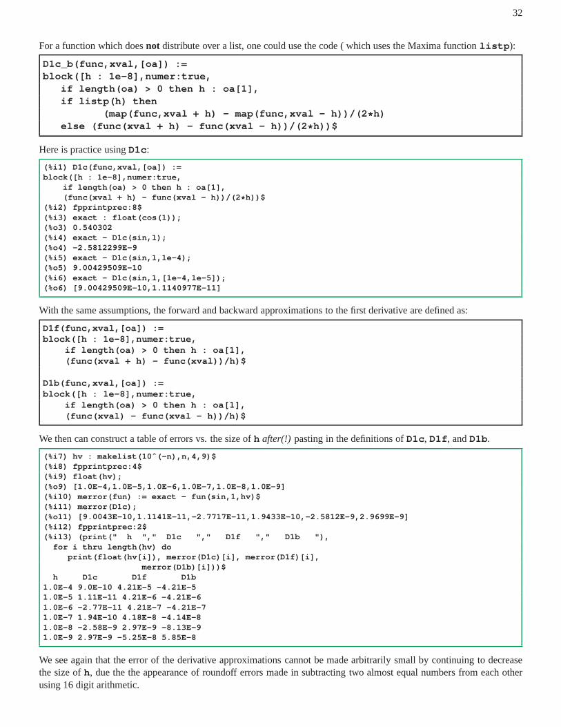
In order to make a table comparing the errors in evaluating the first derivative ofsin(x) at the pointx = 1 , we de-fine the functionsD1c, D1f , andD1b which employ the central, forward, and backward differenceformulas, respectively.
In Rwe had the definition, incorporating a default value ofh if D1c was called with only the first two args supplied:
D1c = function (func, x, h = 1e-8) {(func(x + h) - func(x - h))/(2 * h) }
31
To construct a similar (in result) function in Maxima takes alittle more work. First of all, list arithmetic in Maxima :
However, to incorporate the default value forh, using Maxima, we need to use a special syntax,D1c(func,xval,[oa]) := etc, etc. , which we explain here.
In this Maxima function definition, inside the code,oa (other args) will appear as a list, and the listoa (inside thefunction) will be the zero length list[] if no third arg is supplied, will be a list containing one number [h1] if a numberis supplied for the third arg, and will be a list of a list ofh values if a list is supplied for the third arg. Here is a littletestfunction to explore this behavior:
(%i7) test(func,xval,[oa]) := (print(" oa = ",oa))$(%i8) test(sin,1)$
oa = [](%i9) test(sin,1,1e-4)$
oa = [1.0E-4](%i10) test(sin,1,[1e-2,1e-4])$
oa = [[0.01,1.0E-4]]
The simplest version of Maxima code results from the assumption that the function used in the first slot (func ) distributesover lists in the same way the core functionsin does. We assume, in particular, that homemade functions used with D1cdistribute over lists, in the same way as in these four examples:
We can then avoid the need to usemap to get the function to act on each member of a list, and use the following simplecode (which will do the job in all three cases):
if length(oa) > 0 then h : oa[1],(func(xval + h) - func(xval - h))/(2 * h))$
We see the default value ofh defined in the local variable list at the start of theblock expression. We could just as wellhave used the syntaxblock([h], h:1e-8, etc. to define the default value ofh in the code.
32
For a function which doesnot distribute over a list, one could use the code ( which uses theMaxima functionlistp ):
We see again that the error of the derivative approximationscannot be made arbitrarily small by continuing to decreasethe size ofh, due the the appearance of roundoff errors made in subtracting two almost equal numbers from each otherusing 16 digit arithmetic.
33
1.5 Numerical Quadrature
In Computational Physics, Ch.1, Sec.2, Koonin discusses the trapezoidal rule for a uniform grid, two versions (1/3, 3/8 )of Simpson’s rule for a uniform grid, and Bode’s rule.
When we useRor Maxima to solve complicated physics problems, we will choose the most accurate and efficient meansavailable. If the software available does not have what is needed or what works, homemade functions will be resorted to.The homemade examples for quadrature (trapezoidal and Simpson’s rules) presented here will not necessarily be used inour physics explorations, but understanding how they work will introduce you to theR and Maxima syntax for gettingthings done. We will check the accuracy of these very simple quadrature rules using the quadrature functions available inRand Maxima.
1.5.1 R function integrate for one dimensional integrals
TheR language software has the numerical integration functionintegrate with the syntax
integrate(fun, a, b, ...)
Use of?integrate brings up complete syntax and return named values information. For example, the returned namedvalues info is:
ValueA list of class "integrate" with components
1. valuethe final estimate of the integral.2. abs.errorestimate of the modulus of the absolute error.3. subdivisionsthe number of subintervals produced in the subdivision proc ess.
the default is 100L4. message"OK" or a character string giving the error message.5. callthe matched call.
One can use abbreviations for the names of these returned values. Here are examples of quadrature over a finite interval.
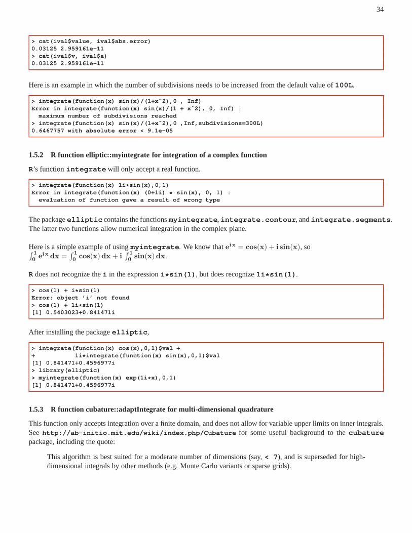
> integrate(sin,0,1)0.4596977 with absolute error < 5.1e-15> fun = function(u) u * sin(u)ˆ2> integrate(fun, 0, 1)0.199694 with absolute error < 2.2e-15> integrate(function(x) sqrt(x) * log(1/x),0,1)0.4444444 with absolute error < 1.3e-07> integrate(function(x) sqrt(x) * log(1/x),0,1,rel.tol = 1e-10)0.4444444 with absolute error < 4.9e-16> ival = integrate(function(x) sqrt(x) * log(1/x),0,1,rel.tol = 1e-10)> cat(ival$value, ival$abs.error, ival$subdivisions, iv al$message)0.4444444 4.934325e-16 8 OK> cat(ival$val, ival$abs.e, ival$sub, ival$mes)0.4444444 4.934325e-16 8 OK> cat(ival$v, ival$a, ival$s, ival$m)0.4444444 4.934325e-16 8 OK
Here is an example of theR function integrate used for an unbounded interval quadrature.
evaluation of function gave a result of wrong type
The packageelliptic contains the functionsmyintegrate , integrate.contour , andintegrate.segments .The latter two functions allow numerical integration in thecomplex plane.
Here is a simple example of usingmyintegrate . We know thatei x = cos(x) + i sin(x), so∫ 1
0ei x dx =
∫ 1
0cos(x)dx + i
∫ 1
0sin(x)dx.
Rdoes not recognize thei in the expressioni * sin(1) , but does recognize1i * sin(1) .
> cos(1) + i * sin(1)Error: object ’i’ not found> cos(1) + 1i * sin(1)[1] 0.5403023+0.841471i
1.5.3 R function cubature::adaptIntegrate for multi-dimensional quadrature
This function only accepts integration over a finite domain,and does not allow for variable upper limits on inner integrals.Seehttp://ab-initio.mit.edu/wiki/index.php/Cubature for some useful background to thecubaturepackage, including the quote:
This algorithm is best suited for a moderate number of dimensions (say,< 7), and is superseded for high-dimensional integrals by other methods (e.g. Monte Carlo variants or sparse grids).
35
To useadaptIntegrate for double or higher multi-dimension integrals, you first need to download the packagecubature . If you are usingRStudio , go to the packages panel and click on ’Install Packages...’.
package cubature successfully unpacked and MD5 sums checke d
The downloaded binary packages are inC:\Documents and Settings\Edwin Woollett\Local Settings \Temp\RtmpGA2HLF\downloaded_packages
You then need to uselibrary to load the package into your current work session. You can then use?name to get thedocumentation and description of required and optional arguments, and (named) return value(s).
> library(cubature)> ?adaptIntegrate
Part of the documentation is:
adaptIntegrate {cubature}Adaptive multivariate integration over hypercubes
Description:The function performs adaptive multidimensional integrat ion
(cubature) of (possibly) vector-valued integrands over hy percubes.
tol = 1e-05, fDim = 1, maxEval = 0,absError=0, doChecking=FALSE)
Arguments:
fThe function (integrand) to be integratedlowerLimitThe lower limit of integration, a vector for hypercubesupperLimitThe upper limit of integration, a vector for hypercubes...All other arguments passed to the function ftolThe maximum tolerance, default 1e-5.fDimThe dimension of the integrand, default 1, bears no
relation to the dimension of the hypercubemaxEvalThe maximum number of function evaluations needed,
default 0 implying no limitabsErrorThe maximum absolute error tolerateddoCheckingA flag to be a bit anal about checking inputs to
C routines. A FALSE value results in approximately9 percent speed gain in our experiments. Yourmileage will of course vary. Default value is FALSE.
36
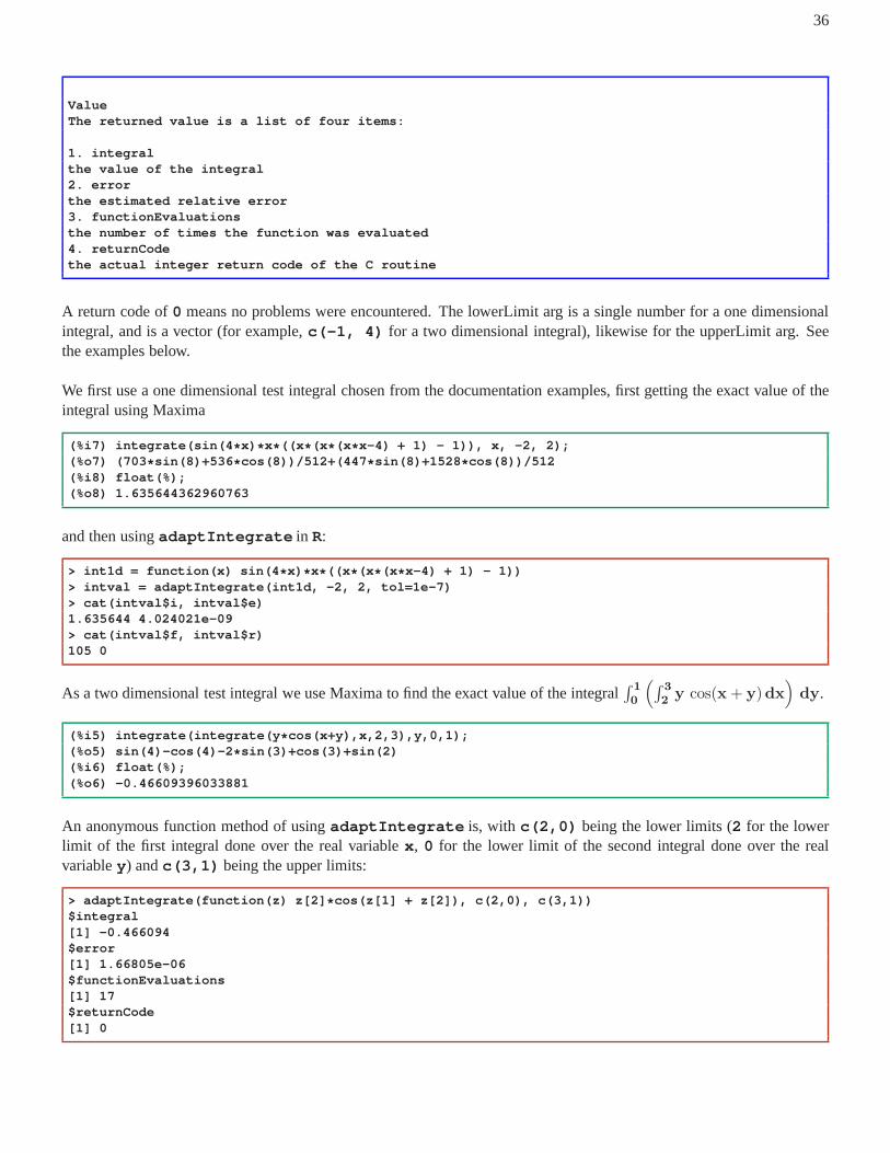
ValueThe returned value is a list of four items:
1. integralthe value of the integral2. errorthe estimated relative error3. functionEvaluationsthe number of times the function was evaluated4. returnCodethe actual integer return code of the C routine
A return code of0 means no problems were encountered. The lowerLimit arg is a single number for a one dimensionalintegral, and is a vector (for example,c(-1, 4) for a two dimensional integral), likewise for the upperLimit arg. Seethe examples below.
We first use a one dimensional test integral chosen from the documentation examples, first getting the exact value of theintegral using Maxima
An anonymous function method of usingadaptIntegrate is, with c(2,0) being the lower limits (2 for the lowerlimit of the first integral done over the real variablex , 0 for the lower limit of the second integral done over the realvariabley) andc(3,1) being the upper limits:
1.5.4 Maxima quadrature functions quadqags and quadqagi
Maxima has various methods for quadrature (see Ch. 8 and 9 ofMaxima by Example on the author’s webpage).
The Maxima functionsquad_qags (for a finite interval) andquad_qagi (for unbounded intervals) require integrandswhich evaluate to real floating point numbers. We discuss their use with complex integrands below.Here is an example of usingquad_qags for finite interval quadrature, taken from the Maxima help manual entry forquad_qags , followed by use of Maxima’sintegrate function which tries to find an exact symbolic value (insteadof an approximate numerical value).
The first element of the list returned byquad_qags is the value of the numerical integral (printed with the number ofdigits related to the current setting offpprintprec ), the second element being an estimate of the size of the absoluteerror of the result, the third element315 being the number of function evaluations, and the last element 0 being theinteger error code, with0 indicating no problems.
Here is an example of using Maxima’squad_qagi for anunbounded interval quadrature.
An example of usingquad_qags for the integration of a complex function. In principle, anycomplex functionf can bewritten asf = fr + %i * fi . We use the Maxima functionsrealpart and imagpart and the integration is done“by hand” by separately integrating the real and imaginary parts, and then combining them at the end.
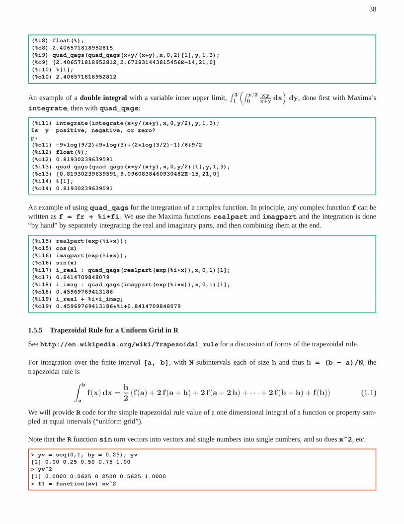
We will provideRcode for the simple trapezoidal rule value of a one dimensional integral of a function or property sam-pled at equal intervals (“uniform grid”).
Note that theR functionsin turn vectors into vectors and single numbers into single numbers, and so doesxˆ2 , etc.
With that background, here is a trapezoidal rule function for a uniform grid. In this code,xv is a R-vector of equallyspaced positions where the function is to be sampled, andyv is aR-vector of function values at those positions.
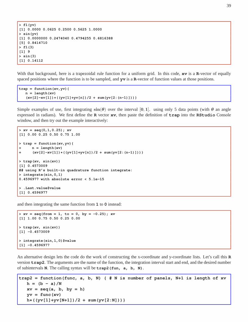
Simple examples of use, first integratingsin(θ) over the interval[0,1]. using only 5 data points (withθ an angleexpressed in radians). We first define theR vectorxv , then paste the definition oftrap into theRStudio Consolewindow, and then try out the example interactively:
> xv = seq(0,1,0.25); xv[1] 0.00 0.25 0.50 0.75 1.00
> trap(xv, sin(xv))[1] 0.4573009## using R’s built-in quadrature function integrate:> integrate(sin,0,1)0.4596977 with absolute error < 5.1e-15
> .Last.value$value[1] 0.4596977
and then integrating the same function from1 to 0 instead:
> xv = seq(from = 1, to = 0, by = -0.25); xv[1] 1.00 0.75 0.50 0.25 0.00
> trap(xv, sin(xv))[1] -0.4573009
> integrate(sin,1,0)$value[1] -0.4596977
An alternative design lets the code do the work of constructing the x-coordinate and y-coordinate lists. Let’s call thisRversiontrap2 . The arguments are the name of the function, the integrationinterval start and end, and the desired numberof subintervalsN. The calling syntax will betrap2(fun, a, b, N) .
trap2 = function(func, a, b, N) { # N is number of panels, N+1 is length of xvh = (b - a)/Nxv = seq(a, b, by = h)yv = func(xv)h* ((yv[1]+yv[N+1])/2 + sum(yv[2:N]))}
1.5.6 Trapezoidal Rule for a Uniform Grid in Maxima
The Maxima analog of anRvector is a Maxima “list”, denoted by square brackets, as in
xv : [1,2,3,4,5,6]
Both Maxima and R usexv[3] to pick out the third element of a vector (third element of a Maxima list). TheMaximafunctionsrest andapply can be used to effect the sum of part of a Maxima list of numbers.
We can use themaxima functionsmakelist andmap to construct a x-coordinate list and then the correspondingy-coordinate list. We can use themaxima parameterfpprintprec to control the number of digits printed to the screen(this does not affect the 16 digit precision of the internal arithmetic).
(%i8) map(sin,[1,2]);(%o8) [sin(1),sin(2)](%i9) float(%);(%o9) [0.8414709848079,0.90929742682568](%i10) makelist(0.25 * i, i, 0, 4);(%o10) [0,0.25,0.5,0.75,1.0](%i11) xv : %;(%o11) [0,0.25,0.5,0.75,1.0](%i12) map(sin, xv);(%o12) [0,0.24740395925452,0.4794255386042,0.6816387 6002333,0.8414709848079](%i13) fpprintprec : 8$(%i14) map(sin, xv);(%o14) [0,0.247404,0.479426,0.681639,0.841471]
We can use themaxima functionquad_qags to do a numerical check ontrap .
with the first element of the return list being the value of thenumerical integral (printed with the number of digits relatedto the current setting offpprintprec ), the second element being an estimate of the size of the absolute error of theresult, the third element (21) being the number of function evaluations, and the last element (0) being the integer errorcode, with0 indicating no problems.
41
You can pick out just the first element of this returned Maximalist using
Once we have constructed the Maxima list to be used for the first (formal) argumentxv , we can either usemap in thefunction call or else pre-define a corresponding coordinatelist to be used for the second (formal) argument oftrap .
We first paste into Maxima (the author uses theXmaxima interface almost exclusively) the definition oftrap . (Notethe crucial delayed assignment symbol:= used to define a Maxima function.) There is one local variabledeclared anddefined inside the local variables bracket[ ] , whose value remains unknown in the global environment. Once you havepasted the definition into XMaxima (usingCtrl+v ), press the keyboard down-arrow key to get to the bottom of theinput, and then pressEnter .
The first example of usingtrap2 uses the name of a function which Maxima knows about (either acore Maxima func-tion, or one defined by a loaded package, or one defined by you with a name prior to callingtrap2 ). The second andthird examples (using the anonymous lambda function) are examples of how you could use your own (unnamed) function.
Integratingsin(x) instead fromx = 1 to x = 0 should reverse the sign, and this is easy to check with versiontrap2 .
1.5.7 Trapezoidal Rule for a Non-Uniform Grid in R
Jarek Tuszynski, in theR packagecaTools , has a version of the trapezoidal rule which can handle unequally spaceddata. (We have replaced hisas.double with as.numeric , since all real floats are treated as double inR, and haveomitted his final wrapreturn() function which is not needed; the last result in a function iswhat is returned (providedthe interior of the function code does not contain areturn() call which is activated by a decision).
Jarek’s code uses the matrix multiply symbol%* %which is used to multiply matrices together, multiply a vector times amatrix, or to multiply two vectors together to form an “innerproduct” of two R-vectors.Rdoes not distinuish row vectorsfrom column vectors; all vectors are equal. The functionsnrow andncol returnNULLfor a vector, while the functionsNROWandNCOLtreat aRvector as a one-column matrix.
For a uniform grid, this reduces to the same algorithm used intrap . We can use small random numbers to deform auniform grid into a non-uniform grid, using thejitter function (which adds a small amount of noise to a vector).
Because each call to the random number generator results in adifferent result, your results forjitter(xv) will notnecessarily be the same as in the above.
1.5.8 Trapezoidal Rule for a Non-Uniform Grid in Maxima
The inner product of two maxima lists is produced by separating the lists by . .
(%i1) [2, 2, 2] . [1, 2, 3];(%o1) 12
Again we use Maxima’smakelist function to produce Maxima code for the non-uniform grid version of the trapezoidalrule.
trapz(xv,yv) :=block([n:length(xv)],
dxx : makelist( xv[i] - xv[i-1], i, 2, n),yy : makelist( yv[i-1] + yv[i], i, 2, n),float(dxx . yy/2))$
After pasting this code into Maxima, we first test this code using a uniform grid as a check.
We now deform the uniform grid using a homemadejitter function in Maxima:
jitter(xv,[o]) :=block([ampl,fac:1],
if not listp(xv) then return("xv must be a list"),if length(o) > 0 then fac : o[1],if length(o) > 1 then ampl : o[2]
else ampl : fac * (apply(max,xv) - apply(min,xv))/50,xv + ampl * makelist(random(2.0) -1, i, 1, length(xv)))$
The syntax isjitter(alist [factor, amplitude]) in which factor and amplitude are both optional argu-ments with default values. The default value of factor is1. To override the default value of factor, usejitter(alist,myfactor) . To override the default value of amplitude, you must have a value in the factor slot also.Here are some simple examples:
(%i7) jitter([1,2,3]);(%o7) [0.997476,2.0216678,3.0163642](%i8) jitter([1,2,3],2);(%o8) [1.0025236,2.0397766,2.9712082](%i9) jitter([1,2,3],1,1/50);(%o9) [0.998108,1.9851285,3.0069044](%i10) jitter(2);(%o10) "xv must be a list"
We now usejitter to deform the previously used uniform grid and again usetrapz :
Note that we assume a “uniform grid”, and the interval of integration is divided into an even number of subintervals, sothe length of the position vectorxv should be odd. A “vectorized”Rcode with similarities totrap above is (withN theeven number of subintervals)
and finally check the error return if the length ofxv is not odd:
> xv = seq(0,1.25, by = 0.25); xv[1] 0.00 0.25 0.50 0.75 1.00 1.25> simp(xv, sin(xv))[1] " length(xv) should be an odd integer "
A secondR language version of Simpson’s rule with the syntaxsimp2(fun, x1, x2, num_panel) requires thecreation of the “position vector”xv inside the function. We then have two ways of usingseq . One method uses theby argument, and the other uses thelength.out argument (which can be shortened tolength ). Here is interactiveexperimentation inR:
> a = 0.5; b = 1.5> N = 4; h = (b-a)/N; h[1] 0.25> seq(a,b,by=h)[1] 0.50 0.75 1.00 1.25 1.50> seq(a,b,length = 5)[1] 0.50 0.75 1.00 1.25 1.50
> simp2(sin,0,1,4)[1] 0.4597077> simp2(sin,1,0,4)[1] -0.4597077> simp2(sin,0,1,5)[1] " N should be an even integer "
1.5.10 Simpson’s 1/3 Rule in Maxima
A straightforward translation of theRversion ofsimp into the Maxima language is:
simp(xv, yv) :=block([n, s],
n : length(xv) - 1, / * number of panels * /if mod(n,2) # 0 then return(" length(xv) should be an odd inte ger "),h : xv[2] - xv[1],if n = 2 then s : yv[1] + 4 * yv[2] + yv[3]else s : yv[1] + yv[n+1] +
(%i12) simp2(sin,0,1,4);(%o12) 0.459708(%i13) simp2(sin,1,0,4);(%o13) -0.459708(%i14) simp2(sin,0,1,5);(%o14) " n should be even number of panels"
1.5.11 Checking Integrals with the Wolfram Alpha Webpage
The Wolfram Alpha web page,http://www.wolframalpha.com , allows free one-line commands (integrals, deriva-tives, plots, etc.,) which may require translating Maxima syntax into Mathematica syntax.
A web page with some translation from Maxima to Mathematica is
http://www.math.harvard.edu/computing/maxima/
A larger comparison of Maxima, Maple, and Mathematica syntax is at
http://beige.ucs.indiana.edu/P573/node35.html
Maxima syntax for 1d symbolic integration over a specified interval is
There is a discussion of these two transformation formulas,on the webpagehttp://ab-initio.mit.edu/wiki/index.php/Cubature in the context of theC implementation of the cubaturecode foradaptIntegral .
Note the Jacobian factors multiplyingf(· · · ) in both integrals, and also that the limits of thet integrals are different inthe two cases.
In multiple dimensions, one simply performs this change of variables on each dimension separately, as desired, multi-plying the integrand by the corresponding Jacobian factor for each dimension being transformed.
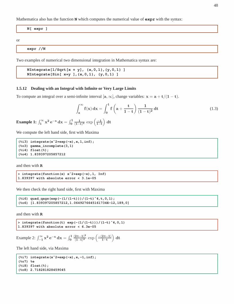
The Jacobian factors diverge as the endpoints are approached. However, iff(x) goes to zero at least as fast as1/x2,then the limit of the integrand (including the Jacobian factor) is finite at the endpoints. If yourf(x) vanishes moreslowly than1/x2 but still faster than1/x, then the integrand blows up at the endpoints but the integral is still finite(it is an integrable singularity), so the code will work (although it may take many function evaluations to converge). Ifyourf(x) vanishes only as1/x, then it is not absolutely convergent and much more care is required even to define whatyou are trying to compute. (In any case, the h-adaptive quadrature/cubature rules currently employed in cubature.c donot evaluate the integrand at the endpoints, so you need not implement special handling for|t| = 1)
50
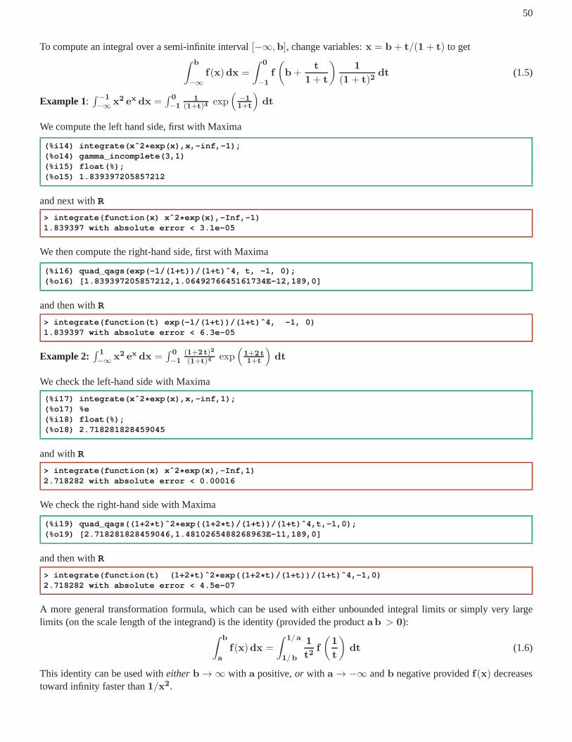
To compute an integral over a semi-infinite interval[−∞,b], change variables:x = b+ t/(1+ t) to get∫ b
A more general transformation formula, which can be used with either unbounded integral limits or simply very largelimits (on the scale length of the integrand) is the identity(provided the productab > 0):
∫ b
a
f(x)dx =
∫ 1/a
1/b
1
t2f
(
1
t
)
dt (1.6)
This identity can be used witheither b → ∞ with a positive,or with a → −∞ andb negative providedf(x) decreasestoward infinity faster than1/x2.
51
For example, one can split the integral∫∞0
f(x)dx =∫ c
0f(x)dx +
∫∞c
f(x)dx, choosing the breakpointc to belarge enough that the asymptotic limit of the integrand is being approached, and then transform thesecond term into∫ 1/c0
1t2
f(
1t
)
dt.
Example takingc = 20:∫∞0
cos(x) e−x dx =∫ 20
0cos(x) e−x dx+
∫∞20
cos(x) e−x dx
and we use the above transformation on the second term to get an integral over a finite domain:∫∞20
cos(x) e−x dx =∫ 1/200
cos(1/t) exp(−1/t)t2
dt.
Using Maxima for the original integral with unbounded limits
we then useR to show that the finite domain transformed term is negligible, and only the first term including contributionsfrom x < 20 needs to be retained.
> integrate(function(t) cos(1/t) * exp(-1/t)/tˆ2,0,0.05)-5.203003e-10 with absolute error < 1.5e-14> integrate(function(x) cos(x) * exp(-x),0,20)0.5 with absolute error < 4.6e-05
This split-up method can be used to evaluate an integral to the precision desired by simply choosingc large enough thatthe neglected piece is small enough compared to the dominantterm over[0, c] .
1.5.13 Handling Integrable Singularities at Endpoints
It is easy to find the integral∫
π
0dx√x=
∫
π
0ddx
(
2√x)
dx = 2√π despite the singularity of the integrand atx = 0. This
is an example of an “integrable singularity”. Likewise Maxima
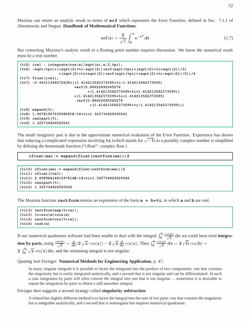
Maxima can return an analytic result in terms oferf which represents the Error Function, defined in Sec. 7.1.1 ofAbramowitz and Stegun:Handbook of Mathematical Functions.
erf(z) =2√π
∫ z
0
e−t2 dt (1.7)
But converting Maxima’s analytic result to a floating point number requires discussion. We know the numerical resultmust be a real number.
The small imaginary part is due to the approximate numericalevaluation of the Error Function. Experience has shownthat reducing a complicated expression involving%i (which stands for
√−1) to a possibly complex number is simplified
by defining the homemade function (“cfloat”: complex float )
If our numerical quadrature software had been unable to dealwith the integral∫ b
0
cos(x)√x
dx we could have triedintegra-
tion by parts, using cos(x)√x
= ddx
(2√x cos(x))− 2
√x d
dxcos(x). Then
∫ b
0
cos(x)√x
dx = 2√b cos(b) +
2∫ b
0
√x sin(x)dx, and the remaining integral is not singular.
Quoting Joel Ferziger:Numerical Methods for Engineering Application, p. 47,
In many singular integrals it is possible to factor the integrand into the product of two components: one that containsthe singularity but is easily integrated analytically, anda second that is not singular and can be differentiated. In sucha case integration by parts will often convert the integral into one that is not singular . . . sometimes it is desirable torepeat the integration by parts to obtain a still smoother integral.
Ferziger then suggests a second strategy calledsingularity subtraction :
A related but slightly different method is to factor the integral into the sum of two parts: one that contains the singularitybut is integrable analytically, and a second that is nonsingular but requires numerical quadrature.
53
Here is a general example:∫ b
0
f(x)√x
dx =
∫ b
0
f(x)− f(0)√x
dx+ f(0)
∫ b
0
dx√x
(1.8)
Applied to our example, this becomes∫ b
0
cos(x)√x
dx =∫ b
0dx√x+
∫ b
0
cos(x)−1√x
dx.
Because(1− x2) = (1− x) (1 + x) → 2 (1− x) asx → 1, the method of singularity subtraction can be used to re-
place the integral∫ 1
0dx√1−x2
by the two terms∫ 1
0
(
1√1−x2
− 1√2 (1−x)
)
dx+∫ 1
0dx√
2 (1−x), in which the second term is
easy to integrate, and the integrand of the first term is smooth asx → 1.
However, both Maxima andRhave no difficulties with this last example, first Maxima:
> integrate(function(x) 1/sqrt(1-xˆ2),0,1)1.570796326786759 with absolute error < 1.7e-06
1.6 Finding Roots
The root of a functionf(x) is the value ofx for which f(x) = 0. In Computational Physics, Ch.1, Sec.3, Koonindiscusses the elementary one variable root finding methods known as the bisection method, the Newton-Raphson method,and the secant method. Seehttp://en.wikipedia.org/wiki/
The coreR functionuniroot , has the syntaxuniroot(func, interval, ...) . Documentation is athttp://127.0.0.1:11976/library/stats/html/uniroot.h tml .
If f is the given function,uniroot searches for a value ofx such thatf(x) is a sufficiently close to zero and returnsthe first suchx . uniroot assumes the given function is continuous in the given interval and that the given function hasat least one root in the interval supplied. That interval is searched starting from the lower end of the interval.
If the given function does not have opposite signs at the endsof the given interval,uniroot returns an error message.
We useuniroot to search for the single root of the equationx2 − 5 = 0 in the interval[1,5]. We can make a simpleplot of the function f(x) = xˆ2 - 5 as follows:
The lwd parameter setting doubles the line width. Theabline statements add a horizontal line aty = 0 to the figurecreated bycurve and then a vertical line atx = 0 to add “axes”. Thelty setting is a line type setting.
uniroot returns a list with four elements: the approximate root location $root , the value of the given function atthe root location found (should be close to zero)f.root , the number of iterations required$iter , and the precisionestimate$estim.prec .
The base code ofRalso includespolyroot , designed to find zeros of a real or complex polynomial.
1.6.3 R function rootSolve::uniroot.all
The rootSolve package functionuniroot.all is a simple extension ofuniroot which extracts many (presumablyall ) roots in the interval. Here is an example taken from Sec.1.1of rootSolve.pdfby Karline Soetaert.
To find the root of functionf(x) = cos3(2x) in the interval[0,8] and plot the curve, we write:
Although the graph (figure 1) clearly demonstrates the existence of many roots in the interval[0,8], the R functionuniroot extracts only one. Here we load the packagerootSolveand useuniroot.all , which finds five roots in thegiven interval. We then place markers in the plot at all theseroots.
. . .uniroot.all does that by first subdividing the interval into small sections and, for all sections where the functionvalue changes sign, invokinguniroot to locate the root.
Note that this is not a full-proof method: in case subdivision is not fine enough some roots will be missed. Also, in casethe curve does not cross the X-axis, but just “touches” it, the root will not be retrieved; (but neither will it be located byuniroot ).
1.6.4 R Newton-Raphson: newton
The Newton-Raphson root finding algorithm is
vk+1 = vk − f(vk)
f ′(vk), (1.9)
To implement this iteration, the symbolic derivative in thedenominator is replaced by a centered numerical derivatives . The initial guessx0 needs to be “close enough” to the root for the Newton-Raphsonalgorithm to be successful. Thecriterion for returning the iteratexn is that the absolute value of the given function evaluated atxn be less thaneps . Wealso want to avoid dividing by zero in a graceful way.
For roots of general functions of one variable, Maxima hasfind_root , bf_find_root , andnewton . The au-thor has also written a bigfloat version of newton, calledbfnewton (see later). For roots of polynomials, Maxima hasrealroots , allroots , andbfallroots .
The Maxima functionfind_root has a behavior which is similar to theR functionuniroot . The documentation forthe Maxima functionsfind_root and the bigfloat versionbf_find_root is (with editing):
find_root (expr, var, a, b, [abserr, relerr])find_root (f, a, b, [abserr, relerr])bf_find_root (expr, var, a, b, [abserr, relerr])bf_find_root (f, a, b, [abserr, relerr])
If the formfind_root(expr,var,...) is used, the symbol used forvar should be the same symbol as is used inexpr . For ex-amplefind_root(yˆ2 - 5, y, 0,5) . find_root finds a root of the expressionexpr or the functionf over the closed in-terval[a, b] . The expressionexpr may be an equation, in which casefind_root seeks a root oflhs(expr) - rhs(expr) .find_root returns an error iff(a) has the same sign asf(b) .
Given that Maxima can evaluateexpr or f over[a, b] and thatexpr or f is continuous,find_root is guaranteed to find theroot, or one of the roots if there is more than one.
find_root initially applies binary search. If the function in question appears to be smooth enough,find_root applies linearinterpolation instead.
bf_find_root is a bigfloat version offind_root . The function is computed using bigfloat arithmetic and a bigfloat re-sult is returned. Otherwise,bf_find_root is identical tofind_root , and the following description is equally applicable tobf_find_root .
The accuracy offind_root is governed by the keywordsabserr and relerr , which are optional keyword arguments tofind_root . These keyword arguments take the formkeyword = value . These keyword arguments are: 1.abserr : De-sired absolute error of function value at root. The default value is the value of the global parameterfind_root_abs .
(%i1) find_root_abs;(%o1) 0.0
2. relerr : Desired relative error of root. The default value is the value of the global parameterfind_root_rel .
(%i2) find_root_rel;(%o2) 0.0
find_root stops when the function in question evaluates to something less than or equal toabserr , or if successive ap-proximantsvar_0 , var_1 differ by no more thanrelerr * max(abs(var_0), abs(var_1)) . The default values offind_root_abs andfind_root_rel are both zero.
find_root expects the function in question to have a different sign at the endpoints of the search interval. When the func-tion evaluates to a number at both endpoints and these numbers have the same sign, the behavior offind_root is governedby find_root_error . Whenfind_root_error is true , find_root prints an error message. Otherwisefind_rootreturns the value offind_root_error . The default value offind_root_error is true .
(%i3) find_root_error;(%o3) true
If expr or f evaluates to something other than a number at any step in the search algorithm,find_root returns a partially-evaluatedfind_root expression.
The order ofa andb is ignored; the region in which a root is sought is[min(a, b), max(a, b)] .
58
In the following examples, we accept the defaultfind_root accuracy parameter values. A simple test of accuracy is tosearch for the positive root of the functionf(x) = x2 − 5, located atxr =
In the first example below, Maxima does not know a value fory , and returns an unevaluated expression (a “noun form” inMaxima-speak). In the second example below, the “variable”in expr is x , and the value of the parametery is suppliedusing the pseudo-postfix notationexpr, param = val .
Here is another example of postfix setting of parameters:
(%i21) x * cos(y) * exp(z),x=2,y=3,z=4;(%o21) 2 * %eˆ4* cos(3)
To solve the last example with 20 digit precision, one needs to set theglobal value offpprec to the value20, and thenusebf_find_root . The functionsbfloat , bf_find_root , andbfallroots (but not float ) compute usingthe number of digits of precision specified by the current value of fpprec . The default value of the global parameterfpprec is 16
If Maxima can symbolically compute the derivative of a givenexpression (function of a single variable) whose root issought, then the Newton-Raphson method can find the root if the initial guess is close enough.
The Maxima help manual refers to contributed code in.../source/numeric/newton1.mac which has the syn-tax newton(expr, var, guess, eps) which returns the current iteration ofvar , sayv , if the absolute value ofexpr , when evaluated atv , is less than the small positive numbereps .
Since the Newton-Raphson iteration rule is
vk+1 = vk − f(vk)
f ′(vk), (1.11)
a “divide-by-zero” error will occur if the first derivative is zero at the current value of the iteration variable.
(%i1) load("newton1.mac");(%o1) "C:/PROGRA˜1/MA81DB˜1.0/share/maxima/5.28.0-2/ share/numeric/newton1.mac"(%i2) newton(xˆ2 - 5,x,1,1e-4);(%o2) 2.236068895643363(%i3) newton(xˆ2 - 5,x,0,1e-4);expt: undefined: 0 to a negative exponent.#0: newton(exp=xˆ2-5,var=x,x0=0,eps=1.0E-4)(newton1. mac line 8)
-- an error. To debug this try: debugmode(true);
A replacementnewton function with the same syntax is in the filecpnewton.macon the author’s webpage with thischapter and the contents include an exprerimental bigfloat version too.
The syntax ofbfnewton is bfnewton(expr, var, guess, digits) , in whichdigits is the requested pre-cision of the returned root. The value offpprec is set (locally) to a value higher thandigits . There is no need tochange the global setting offpprec . This is an experimental version of Newton-Raphson.
Here we usebfnewton , already loaded in with the filemynewton.mac , to find the positive root of the functionxˆ2 - 5 to 20 digit accuracy.
In the last two inputs, using a local setting offpprec andbfloat inside ablock expression, we compared the rootfound,r20 , with the “exact value”exact , and evaluated the function at the position of the root found.
Here we check the zero derivative error case:
(%i10) bfnewton(xˆ2 - 5,x,0,20);derivative at 0.0b0 is zero
(%o10) " bfnewton failed"
61
1.6.9 Maxima function secant
The secant root finding algorithm is
vk+1 = vk − f(
vk) vk − vk−1
f (vk)− f (vk−1)(1.12)
The secant method requires two initial guessesx0 and x1 to get started. The syntax issecant(f,x0,x1) orsecant(f,x0,x1,eps) , in which f is either a known function or else alambda form as shown in the secondexample below.
In Computational Physics, Sec. 1.3, Koonin presents a “surefire method” of finding the root of a function when the ap-proximate location of the root is known. (This method cannotfind a root in which the function dips down to touch thexaxis somewhere but doesn’t cross the axis.)
You guess a trial value ofx guaranteed to be less than the root, “increase this trial value by small positive steps, backingup and halving the step size every time the function changes sign.” When the value of the step sizedx is less than somesmall number, the search returns with the finalx value found.
Here is aR function rtsearch which implements this method.
if (abs(dx) <= xacc) breakx = x + dxif (fold * func(x) < 0) {
x = x - dxdx = dx/2}}
x}
After pasting in this definition ofrtsearch into theRConsole, we use it to do a brute force search for the positive rootof the functionfnf(x) = x2 − 5.
mtext {graphics} R DocumentationWrite Text into the Margins of a Plot
Description: Text is written in one of the four margins of the current figureregion or one of the outer margins of the device region.
Usage:mtext(text, side = 3, line = 0, outer = FALSE, at = NA,
adj = NA, padj = NA, cex = NA, col = NA, font = NA, ...)
Arguments:
1. text: a character or expression vector specifying the tex t to be written.Other objects are coerced by as.graphicsAnnot.
2. side: on which side of the plot (1=bottom, 2=left, 3=top, 4 =right).
3. line: on which MARgin line, starting at 0 counting outward s.
4. outer: use outer margins if available.
5. at: give location of each string in user coordinates. If th e component of atcorresponding to a particular text item is not a finite value (the default),
the location will be determined by adj.
6. adj: adjustment for each string in reading direction. For strings parallelto the axes, adj = 0 means left or bottom alignment, and adj = 1 m eans
right or top alignment.
If adj is not a finite value (the default), the value of par("l as")determines the adjustment. For strings plotted parallel to the axisthe default is to centre the string.
7. padj: adjustment for each string perpendicular to the rea ding direction(which is controlled by adj). For strings parallel to the axe s,padj = 0 means right or top alignment, and padj = 1 means left or bottom alignment.
If padj is not a finite value (the default), the value of par(" las") determinesthe adjustment. For strings plotted perpendicular to the ax is the default is tocentre the string.
8. cex: character expansion factor. NULL and NA are equivale nt to 1.0. This is anabsolute measure, not scaled by par("cex") or by setting par ("mfrow")
or par("mfcol"). Can be a vector.
9. col: color to use. Can be a vector. NA values (the default) m ean use par("col").
10. font: font for text. Can be a vector. NA values (the defaul t) mean use par("font").
11 ... Further graphical parameters (see par), including fa mily, las and xpd.(The latter defaults to the figure region unless outer = TRUE , otherwise
the device region. It can only be increased.)
Details
The user coordinates in the outer margins always range from z ero to one, and are notaffected by the user coordinates in the figure region(s) R di ffers here from otherimplementations of S.
64
All of the named arguments can be vectors, and recycling will take place to plot asmany strings as the longest of the vector arguments.
Note that a vector adj has a different meaning from text. adj = 0.5 will centre thestring, but for outer = TRUE on the device region rather than t he plot region.
Parameter las will determine the orientation of the string( s). For strings plottedperpendicular to the axis the default justification is to pl ace the end
of the string nearest the axis on the specified line. (Note th at thisdiffers from S, which uses srt if at is supplied and las if it is not.Parameter srt is ignored in R.)
Note that if the text is to be plotted perpendicular to the axi s, adj determinesthe justification of the string and the position along the ax is unless at is specified.
Graphics parameter "ylbias" (see par) determines how the te xt baseline is placedrelative to the nominal line.
Side Effects
The given text is written onto the current plot.
See Also: title, text, plot, par; plotmath for details on mat hematical annotation.
You can see the current setting ofmar usingpar()$mar . You can see the current setting ofomausingpar()$oma . Youcan change settings using
The following figure1.R script uses zero outer margin area (the default).
In the text command, the optioncex=3 asks for triple the normal text size.
In the mtext command,side=1 andadj=1 asks for right justified text in the bottom margin of the figure(use ofadj=0.5 would place the text in the bottom center margin), andcex=2 asks for double the default text size. The optionline=3 to themtext commmand asks that the text be positioned starting at three text lines below the plot region.
Loading and executing this script inRshows that the blue box drawn around the figure does not show upin theRConsoleplot, butdoes show up in the LaTeX/dvi display offigure1.eps .
> source("figure1.R")
as shown on the next page.
65
Here is the resulting plot:
0 2 4 6 8 10
02
46
810
X
Y PlotArea
Figure
Figure 7: Default No Outer Margin Area
The LaTeX code for this plot was
\smallskip\begin{figure} [h]
\centerline{\includegraphics[scale=.5]{figure1.eps} }\caption{Default No Outer Margin Area}
\end{figure}
and makes use of thegraphicx LaTeX package.
Quoting Earl F. Glynn (Stowers Institute of Medical Research) on the webpagehttp://research.stowers-institute.org/efg/R/Graphic s/Basics/mar-oma/(with some light editing)
In Figure 1 the “plot area” is inside the red box, and the perimeter of the figure is shown in a blue box . . . The areabetween the red box and the blue box is known as the “margin” area, and is controlled by theR mar parameter. Youcan view the value ofmar at any time from theRcommand line:par()$mar produces[1] 5.1 4.1 4.1 2.1 .
You can set themar parameter to other values using thepar function, as inpar(mar=c(4, 4, 2, 0.5)) . Notethat even though the margin is measured in “lines”, the values need not be integers.
There is no “outer margin area” in this simple example, whichis typical of manyRplots.
In the next example, an “outer margin area” is added, and messages are placed in that area usingmtext . The script filefigure2.R is
mtext(Margins, North <- 3, line=2, adj=0, cex=1.5, col="bl ue")
which, indeed gives the same result, because the second default arg tomtext is the value of the optionside (whichdefaults to 3, implying the top).
67
This is a case in which onemust use<- instead of=, becauseR interprets a function argument of the formkeyword = value differently from the formname <- value . In the former case,Rfinds a keyword it is ready touse and the equal sign is taken to mean: set the keyword to thatvalue. In the latter case, thename is assigned the value,the namebecomes a number, and since it appears in the second slot ofmtext , it is taken to be the desired value of thekeywordside .
It is certainly true that, when reading code,South <- 1 is more readily translated mentally to “that is going on thebottom of the figure”.
Note thatasp returns to its default settingNULLafter usingsource with the graphics filecircle2.R .
Running this script produces:
−1.0 −0.5 0.0 0.5 1.0
−1.
0−
0.5
0.0
0.5
1.0
x
y
Figure 9: homemade circles
1.8.2 Circles Using the R Package shape
Theshapepackage by Karline Soetaert includes functions to create anempty starting plot withasp = 1 as the default,and to draw ellipses, circles, cylinders, arrows, and rounded rectanges with and without color.
to respectively load theshape package, see html documentation of the available functions, and peruse a pdf giving someexamples of some of the functions together with the graphic results.
We will restrict ourselves toemptyplot andplotcircle .
emptyplot has the syntax and defaults:
emptyplot(xlim = c(0, 1), ylim = xlim, asp = 1, frame.plot = FA LSE,col = NULL, ...)
which sets up a plot region without axes or frame, with no background color, and with the plotting region extending fromx=0,y=0 to x=1,y=1 . Thus, usingemptyplot() without supplying any arguments would accept all these defaultsettings.
with a default radius of one unit, a default center of the circle located atx=0,y=0 , a full circle is drawn as a line witha slightly thicker style in a black color, with no fill (color)added, and with no arrow added. Note especially thatlcoldetermines the line color, andcol determines the fill color. Thus the two commands:
> emptyplot()> plotcircle()
will produce an empty black quarter circle showing only thex > 0, y > 0 quadrant.