JOURNAL OF ECONOMIC DEVELOPMENT 33 Volume 38, Number 3, September 2013 CONDITIONAL VOLATILITY ASYMMETRY OF BUSINESS CYCLES: EVIDENCE FROM FOUR OECD COUNTRIES KIN-YIP HO a , ALBERT K. TSUI b AND ZHAOYONG ZHANG c * a The Australian National University, Australia b National University of Singapore, Singapore c Edith Cowan University, Australia Most studies of business cycle exclude the dimension of asymmetric conditional volatility. In this paper, we propose three bivariate asymmetric GARCH models to capture the properties of conditional volatility and time-varying conditional correlations of business cycle indicators in four OECD countries. Our study extends the constant conditional correlation framework proposed by Bollerslev (1990) and the time-varying conditional correlation approach by Tse and Tsui (2002), respectively. Using indices of industrial production as proxies for business cycles indicators, we detect statistically significant evidence of asymmetric conditional volatility in the UK and US. Additionally, we find that the conditional correlations are significantly time-varying, and that the strength of varying correlations may be linked to the degree of economic integration between the countries. Keywords: Business Cycle Non-Linearities, Constant Correlations, Index of Industrial Production, Multivariate Asymmetric GRACH, Varying-Correlations JEL classification: E32, E37 1. INTRODUCTION In the past two decades various approaches to studying properties of the business cycle indicators have been conducted by researchers such as Neftci (1984), Luukkonen and Terasvirta (1991), Terasvirta and Anderson (1992) and Sichel (1989). Basically * The authors wish to thank the anonymous referees for their very helpful comments and suggestions. The first author would like to acknowledge the support provided by Korea Institute for International Economic Policy (KIEP) Visiting Fellowship Program, Accounting and Finance Association of Australia and New Zealand (AFAANZ) Grant, ANU College of Business and Economics Grants, and Research School of Finance, Actuarial Studies and Applied Statistics Grants. The third author wishes to acknowledge the financial support of a strategic research grant from ECU.
Transcript
JOURNAL OF ECONOMIC DEVELOPMENT 33 Volume 38, Number 3, September 2013
CONDITIONAL VOLATILITY ASYMMETRY OF BUSINESS CYCLES:
EVIDENCE FROM FOUR OECD COUNTRIES
KIN-YIP HO
a, ALBERT K. TSUI
b AND ZHAOYONG ZHANG
c*
aThe Australian National University, Australia bNational University of Singapore, Singapore
cEdith Cowan University, Australia
Most studies of business cycle exclude the dimension of asymmetric conditional volatility. In this paper, we propose three bivariate asymmetric GARCH models to capture the properties of conditional volatility and time-varying conditional correlations of business cycle indicators in four OECD countries. Our study extends the constant conditional correlation framework proposed by Bollerslev (1990) and the time-varying conditional correlation approach by Tse and Tsui (2002), respectively. Using indices of industrial production as proxies for business cycles indicators, we detect statistically significant evidence of asymmetric conditional volatility in the UK and US. Additionally, we find that the conditional correlations are significantly time-varying, and that the strength of varying correlations may be linked to the degree of economic integration between the countries. Keywords: Business Cycle Non-Linearities, Constant Correlations, Index of Industrial
1. INTRODUCTION In the past two decades various approaches to studying properties of the business
cycle indicators have been conducted by researchers such as Neftci (1984), Luukkonen and Terasvirta (1991), Terasvirta and Anderson (1992) and Sichel (1989). Basically
* The authors wish to thank the anonymous referees for their very helpful comments and suggestions. The
first author would like to acknowledge the support provided by Korea Institute for International Economic
Policy (KIEP) Visiting Fellowship Program, Accounting and Finance Association of Australia and New
Zealand (AFAANZ) Grant, ANU College of Business and Economics Grants, and Research School of
Finance, Actuarial Studies and Applied Statistics Grants. The third author wishes to acknowledge the
financial support of a strategic research grant from ECU.
KIN-YIP HO, ALBERT K. TSUI AND ZHAOYONG ZHANG 34
these studies concentrate on the asymmetric and non-linear features of business cycles incorporated into the conditional mean equation rather than the conditional variance formulation. To the best of our knowledge, Hamori (2000) is the only empirical study of asymmetry in the volatility shocks of business cycle indicators. More specifically, Hamori (2000) applies the exponential generalized autoregressive conditional heteroskedastic (EGARCH) model proposed by Nelson (1991) on the real GDP growth rates of Japan, UK and US. He finds no statistically significant evidence of volatility asymmetry. Recently, the hypothesis of volatility asymmetry in business cycle indicators is re-examined by Ho and Tsui (2003 and 2004) using univariate asymmetric power ARCH (APARCH) and EGARCH models. In contrast, they detect significant asymmetric effects in the highly developed countries like Canada, UK and US, and also in the relatively less developed countries like Hong Kong, Taiwan and China, respectively. Apparently, it is premature to conclude with an absence of asymmetric volatility in growth rates of GDP.
The main drawback of univariate GARCH analysis is that it fails to capture the co-movement of macroeconomic variables. However, these co-movement relationships are important issues emphasised by the business cycle researchers. For example, Lucas (1977) underscores the significance of examining co-movements of a country’s main macroeconomic indicators such as production, consumption and employment. More recently, Diebold and Rudebusch (1996) argue that business cycle models should take into account the co-movement of macroeconomic variables and their regime-switching behaviour.1 In addition, features of international co-movements and transmission of business cycles have also received much attention recently (see Frankel and Rose, 1998; A’Hearn and Ulrich, 2001; and Choe, 2001). These studies, however, mainly focus on formulating ad-hoc structures to capture co-movements of certain macroeconomic variables. Little work has been done on formally modelling co-movements of asymmetric conditional volatilities in the context of multivariate GARCH setting.
In this paper, we propose three new bivariate asymmetric GARCH models to accommodate the individual conditional heteroskedastic effects and the possibly varying conditional correlation relationships of asymmetric volatilities of the business cycles indicators in the selected OECD countries including Canada, Italy, the UK and the US. In particular, we extend the work by Ding et al. (1993), Sentana (1995), and Tse and Tsui (2002) to incorporate the possibly asymmetric effects of the business cycles shocks on a specific country. This study has important implications. First, if business cycles are conditionally heteroskedastic and exhibit volatility asymmetry, then any theory without such properties is inadequate. Second, the GARCH structure is consistent with the hypothesis of rational expectations in macroeconomics as rational economic agents make decisions based on all available information (see Hong and Lee, 2001 for details). Third, since movements in the financial markets are inextricably linked to the overall
1 See also Hsu and Kuan (2001) for a detailed discussion.
CONDITIONAL VOLATILITY ASYMMETRY OF BUSINESS CYCLES 35
health of the economy, adequate accommodation of macroeconomic uncertainty such as conditional volatilities of business cycles would help researchers understand more about the causes of changes in financial market volatilities. Fourth, it is vital to understand the domestic macroeconomic policy implications of asymmetric volatility and the corresponding policy co-ordinations among major international trading partners.
The rest of the paper is organized as follows. Section 2 explains the methodology of the proposed models and their advantages. Section 3, after describing the data used in this study, highlights some empirical issues and presents the estimation results. Section 4 provides some concluding remarks.
2. BIVARIATE ASYMMETRIC GARCH MODELS The success of Engle’s (1982) ARCH and Bollerslev’s (1986) GARCH models in
characterising volatility dynamics has motivated researchers to make extensions to the multivariate context. The major problem with multivariate generalisation is that the number of parameters to be estimated is inevitably increased, thereby complicating specifications of the conditional variance-covariance matrix (see Bera and Higgins, 1993; and Tse, 2000). To ensure the variance and covariance matrix is positive-definite, Engle and Kroner (1995) propose the BEKK model. One disadvantage of this model is that the parameters cannot be easily interpreted, and their net effects on the conditional variances and co-variances are not readily apparent. More recently, Tse and Tsui (2002) develop a varying-correlation MGARCH (VC-MGARCH) model to incorporate dynamic correlations and yet satisfy the positive-definite condition. One major advantage of VC-MGARCH is that it retains the usual interpretation of the univariate GARCH equation and is more manageable than that of the BEKK model. In addition, the VC-MGARCH model nests a constant-correlation MGARCH (CC-MGARCH) model and therefore provides an indirect way of testing the constant correlations hypothesis. Moreover, Tse and Tsui (2002) report that the VC-MGARCH model compares favourably against the BEKK model based on some empirical studies of the Singapore and Hong Kong stock markets. However, the VC-MGARCH approach does not explicitly model the possible existence of volatility asymmetry, whereby a negative return shock may generate greater impact on future volatilities compared with a positive shock of the same magnitude. To rectify such discrepancies, we propose three new bivariate asymmetric GARCH models based on a synthesis of the methodologies of Ding et al. (1993), Sentana (1995) and Tse and Tsui (2002). They are, namely, the VC-Quadratic GARCH (VC-QGARCH) model, the VC-Leveraged GARCH (VC-LGARCH) model, and the VC-Threshold GARCH (VC-TGARCH) model, respectively. These specifications enable the concurrent modelling of conditional volatility asymmetry and time-varying conditional correlations. They also nest various popular versions of asymmetric GARCH models. As little study has been concentrated on co-movements of the conditional heteroskedasticity of macroeconomic variables, we
KIN-YIP HO, ALBERT K. TSUI AND ZHAOYONG ZHANG 36
shall apply the proposed models to examine the possible evidence of volatility asymmetry and time-changing conditional correlation in the overall Index of Industrial Production (IIP) of Canada, Italy, the United Kingdom and the United States, respectively.
Denoting itY as the ith variable of interest, we define the growth rate (in percentage)
computed on a continuously compounding basis as
100)log(1
it
itit
Y
Yy . (1)
We assume that the conditional mean equation for each variable is effectively
captured by an autoregressive filter of order k:
itjit
k
jiit εyππy
10 , (2)
where itε is the identically and independently distributed error term. The structure of
itε is set up as
ititit esε , where )1,0(~ Neit . (3)
Note that its is associated with the conditional variance equation under three
different specifications, namely, the QGARCH, LGARCH and TGARCH models, respectively. These specifications are less restrictive since they nest several versions of popular GARCH models.
The QGARCH(1,1) model proposed by Sentana (1995) is specified as
12
11 itititit sαεγεηs , (4)
where γ is the asymmetric coefficient. It represents the most general quadratic version
possible within the ARCH class and encompasses many existing quadratic variance functions. The QGARCH model provides a very neat way of calibrating and testing for dynamic asymmetries in the conditional variance function without departing significantly from the standard specification.
The LGARCH and TGARCH models proposed by Ding et al. (1993) share the following structure:
δit
δitit
δit sβγεεαηs 111 )( . (5)
CONDITIONAL VOLATILITY ASYMMETRY OF BUSINESS CYCLES 37
When 2δ , this is the LGARCH(1,1) model which nests the GJR specification.2 According to Engle and Ng (1993), the GJR formulation is the best parametric model compared with other models like EGARCH. Alternatively, when 1δ , it becomes the TGARCH(1,1) model, which incorporates an asymmetric version of the Taylor/Schwert model and Zakoian’s (1994) Threshold ARCH (TARCH) model.
Intuitively, the VC-MGARCH model proposed by Tse and Tsui (2002) has a time-varying conditional correlation structure resembling a standard Box-Jenkins type of ARMA structure. In particular, the conditional correlations formulation in a bivariate VC-MGARCH model is
121121 )1( ttt ψθρθρθθρ , (6)
where ρθθ )1( 21 is the time-invariant conditional correlation coefficient, 1θ and
2θ are assumed to be nonnegative and sum up to less than 1, and 1tψ is specified as
))(( 2,2
21
2,1
21
,2,12
11
ntnntn
ntntnt
ee
eeψ . (7)
Ignoring the constant term and assuming normality, the conditional log likelihood
function of the sample of size n is
t t
tttttt
ρ
eeρeeρL
)1(
2)1log(
2
12
,2,12,2
2,12 . (8)
The total number of parameters is 11 for a bivariate asymmetric GARCH model with
varying correlations, and this number always exceeds that of Bollerslev’s (1990) constant-correlation model by 2. In fact, the CC-MGARCH model is nested within the VC-MGARCH model by restricting 1θ and 2θ to 0.
2 The generalized version of the GJR model (Glosten, Jagannathan, and Runkle, 1993) can be specified as
2
1
2
1
02 )( jt
p
j
jitiit
q
i
it sβεγεαηs
.
KIN-YIP HO, ALBERT K. TSUI AND ZHAOYONG ZHANG 38
3. EMPIRICAL ANALYSIS
3.1. The Data Our data sets comprise 444 monthly indices of industrial production (IIP) series for
Canada, Italy, the United Kingdom and the United States. These seasonally adjusted data sets are culled from the OECD website (source OECD: Main Economic Indicators), covering the period from January 1961 to December 1997. The four series are also obtainable from IMF International Financial Statistics CD-ROM. We apply the same methodology to both data sets and find consistent estimation results. As such, only the findings based on the OECD sources are reported in this paper. There are four reasons to justify the preference of IIP to GDP as proxies for business cycle indicators. First, IIP series is widely used by many researchers (see Blanchard and Quah, 1989; Terasvirta and Anderson, 1992; A’Hearn and Woitek, 2001; and Hsu and Kuan, 2001). Second, according to OECD’s Main Economic Indicators, the series is used as the major reference for aggregate economic activity in Canada, Italy, the United Kingdom and the United States. Prompt availability of the series on a monthly basis and its closely related cyclical profiles with GDP are the main reasons for its popularity. Third, the chosen four OECD countries have included mining, manufacturing, and electricity, gas and water in IIP series, thereby ensuring comparability of data sets across countries. In contrast, not all OECD countries have implemented the System of Nation Accounts (SNA) promulgated by the United Nations in 1993 as the basis for compiling GDP figures.3 For example, real GDP estimates produced by the US are of the chain volume type, whereas those by Canada and UK are based on the more traditional fixed-base volume estimates. Hence, one should avoid such aberrations that may affect the related estimation and statistical inference. Finally, a larger data set is required to facilitate computational convergence in the estimation of model parameters. On balance, the monthly IIP series are preferred to the quarterly GDP as reasonable proxies for the business cycles indicators.
As shown in Table 1, all growth rates of IIP series (in percentage) are negatively skewed and leptokurtic. In particular, the UK has the highest kurtosis, about 3 times than that of a standard normal distribution. On the other hand, the skewness is highest for the US, indicating that negative growth rates are more prevalent. Such non-normal properties are also captured by the highly significant Jarque-Bera test statistics reported in Panel B. As such, appropriate GARCH models seem adequate to accommodate the statistical feature of leptokurtosis.
3 See OECD’s (2001) National Accounts of OECD Countries for reference.
CONDITIONAL VOLATILITY ASYMMETRY OF BUSINESS CYCLES 39
Table 1. Summary Statistics of IIP Growth Rates Country Canada Italy United Kingdom United States
Panel A: Moments, Maximum, and Minimum Mean 0.0030 0.0028 0.0014 0.0030 Median 0.0030 0.0033 0.0013 0.0038 Maximum 0.0403 0.1266 0.0934 0.0334 Minimum -0.0384 -0.1600 -0.0822 -0.0426 Standard Deviation 0.0113 0.0247 0.0149 0.0081 Skewness -0.2403 -0.2091 -0.1942 -0.6888 Kurtosis 3.5309 9.1857 12.1659 6.5276 Observations 444 444 444 444
Panel B: Jarque-Bera Test Test Statistic 9.4652 709.4868 1553.5290 264.7188
Panel H: QARCH LM Test 1 lag 2.8880 57.6593 98.3684 89.5156 4 lags 23.2095 100.6285 150.2096 100.3844
Notes: 1. The Jarque-Bera test statistic follows the chi-squared distribution with 2 degrees of freedom, whilst
the Ljung-Box Q-statistic, the McLeod-Li, and the ARCH LM test statistics follow the chi-squared
distribution with degrees of freedom equal to the number of lags. 2. For the BDS test, e represents the
embedding dimension whereas l represents the distance between pairs of consecutive observations, measured as a multiple of the standard deviation of the series. 3. 1R for 3,2,1i denote the runs tests of the series
tR , tR , and 2tR respectively. Under the null hypothesis that successive observations in the series are
independent, the test statistic is asymptotically standard normal. 4. The QARCH(q) LM test statistic (Sentana,
1995) follows a chi-squared distribution with q(q+3)/2 degrees of freedom.
KIN-YIP HO, ALBERT K. TSUI AND ZHAOYONG ZHANG 40
The applicability of GARCH models is further reinforced by the detection of conditional heteroskedasticity. As indicated in Panel D of Table E, the McLeod-Li and the ARCH LM test results are significant at the 5% level. In addition, the non-parametric BDS and Runs tests are conducted as diagnostic checks. It is noted that the BDS test proposed by Brock et al. (1996) has power against a variety of possible deviations from independence. As can be observed from Panels F and G, the BDS tests unequivocally reject the hypothesis that IIP series are identically and independently distributed. The Runs tests based on the squared and absolute series of the growth rates of Italy, UK and US are statistically significant at the 5% level, indicating the presence of conditional heteroskedasticity.
The observed features of IIP series are similar to those of GDP series reported by Hamori (2000), and Ho and Tsui (2003 and 2004). They all note that UK has the highest kurtosis of real GDP growth rates among the other OECD countries, while that of the US is negatively skewed. Also, Ho and Tsui (2003 and 2004) report highly significant BDS tests for all GDP series in their studies. However, we observe that the kurtosis of IIP series is even larger than that of GDP series for the same country. For example, the kurtosis of GDP growth rates in Canada, the UK and the US are 2.919, 6.033, and 3.983, respectively, whereas the corresponding values of IIP series are 3.531, 12.166, and 6.528. This may be due to the larger sample size of IIP series in our study, or due to the possibility that industrial production is more likely to be affected by irregular events in a monthly frequency.
Finally, Panel H of Table 1 displays the QARCH(q)-LM test statistics, which are
computed by regressing the squared growth rate ( 2tr ) on a constant, the first q lags of
2tr , the cross products of the form jtit rr , and the first q lags of the growth rate tr ,
respectively. Except for Canada, the LM tests for Italy, UK and US are all significant at the 5% level, indicating the presence of asymmetric conditional volatilities. We also launch a more powerful one-sided QARCH(q)-LM test proposed by Sentana (1995), which is constructed by summing up squares of t-ratios of the respective regression coefficients. Though not reported here, the test results are similar to those of the two-sided LM tests. We have also conducted the augmented Dickey Fuller (ADF) and Phillips-Perron (PP) tests to ensure that our data sets are stationary. The Ljung-Box Q-statistic and the Breusch-Godfrey (BG) diagnostic checks for residuals obtained from the ADF regression equation are statistically insignificant at the 5% level, implying that the residuals are approximately white noise (the results are available upon request).
3.2. Estimation Results and Discussions Tables 2-4 report the estimation results of the VC-QGARCH, VC-LGARCH, and
VC-TGARCH models. Figures 1-3 present the results of the conditional correlations of IIP of these countries. First, the estimated coefficient of volatility asymmetry is significant at the 5% level for Canada, the UK, and the US in all three models. For the
CONDITIONAL VOLATILITY ASYMMETRY OF BUSINESS CYCLES 41
UK and the US, the estimated coefficients suggest that negative shocks have a greater impact on future volatilities than positive shocks of the same magnitude.4 Second, the estimated coefficient of volatility asymmetry for Canada indicates that positive rather than negative shocks of IIP growth rates increase future volatilities. This is inconsistent with Ho and Tsui (2003 and 2004). They find that negative rather than positive shocks to GDP growth rates have a greater impact on Canada’s real GDP volatility. Intuitively, as the cyclical profiles of IIP and real GDP are closely related, both should yield similar results. However, IIP and real GDP series do not comprise identical components. Unlike IIP, real GDP contains some sluggish components such as the agriculture and services. In the case of a large service sector in GDP, the output will most likely not be accurately measured. As Canada has a large agricultural products sector, her output may be dominated by the meteorological cycles, thereby yielding inaccurate measurement. As such, findings on the significance and signs of the asymmetric coefficients could differ. Regardless of the discrepancy in signs, our results provide evidence that it is premature to conclude that business cycle indicators do not exhibit volatility asymmetry.
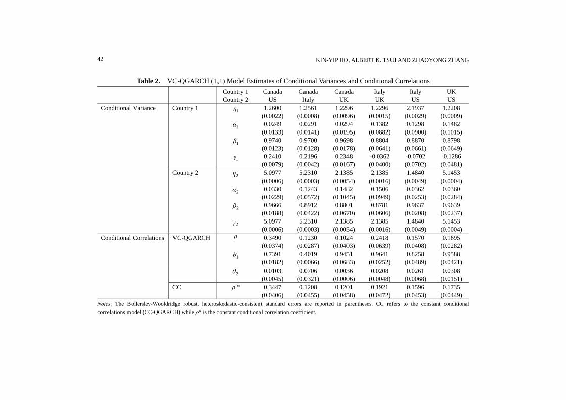
Most parameter estimates of the time-varying conditional correlation coefficient equation are significant at the 5% level, indicating that dynamic correlations probably exist among the 4 OECD countries. Additionally, the estimates of the time-invariant component of the correlation coefficient () are significantly positive and broadly similar to those estimates from the constant conditional correlations models. The finding of positive correlations is consistent with other empirical studies such as Choe (2001), who observes that in an equilibrium-business cycle framework, the international co-movement of cyclical variation in income is positively correlated across countries.
More importantly, the pattern of conditional correlations and the magnitudes of estimated differ among the 6 country pairs permuted from the four OECD countries. For instance, in the case of the VC-QGARCH model, the estimated is 0.3490 for the Canada-US pair, whereas it is 0.1230 for the Canada-Italy pair. In general, the estimated is the highest when the US is combined with Canada and lowest when combined with Italy. This is consistent with results from the VC-LGARCH model. Also, the VC-TGARCH model suggests that the correlation between Canada and US is stronger than the Canada-Italy and US-UK pairs. One possible explanation is the different levels of economic integration and bilateral trade intensities between two trading partners. Indeed, Frankel and Rose (1998) have found that OECD countries with closer trade links tended to have more tightly correlated business cycles. According to the 2002 Index of Economic Freedom, the US is Canada’s top export and import trading partner, accounting for 86.1% and 73.7% of Canada’s exports and imports respectively.
4 Ho and Tsui (2003) have detected significantly negative volatility asymmetry in the real GDP of the US,
and Bodman (2009) finds evidence of significant business-cycle effects, including leverage effects and
asymmetries in the case of Australia.
KIN-YIP HO, ALBERT K. TSUI AND ZHAOYONG ZHANG 42
Table 2. VC-QGARCH (1,1) Model Estimates of Conditional Variances and Conditional Correlations
Country 1 Canada Canada Canada Italy Italy UK Country 2 US Italy UK UK US US Conditional Variance Country 1 1η 1.2600
Notes: The Bollerslev-Wooldridge robust, heteroskedastic-consistent standard errors are reported in parentheses. CC refers to the constant conditional
correlations model (CC-TGARCH) while * is the constant conditional correlation coefficient.
CONDITIONAL VOLATILITY ASYMMETRY OF BUSINESS CYCLES 45
Figure 1. Conditional Correlations of IIP of 4 OECD Countries under VC-QGARCH
KIN-YIP HO, ALBERT K. TSUI AND ZHAOYONG ZHANG 46
Figure 2. Conditional Correlations of IIP of 4 OECD Countries under VC-LGARCH
CONDITIONAL VOLATILITY ASYMMETRY OF BUSINESS CYCLES 47
Figure 3. Conditional Correlations of IIP of 4 OECD countries under VC-TGARCH
Also, the US Department of Commerce’s Survey of Current Business July 1999 has highlighted that Canada is the top trading partner of the US. Based on the Economic Cycle Research Institute (ECRI)’s chronology, almost all the growth rate cycle peaks and troughs of Canada and the US coincide with each other. For instance, during 1960-1997, 9 peaks in the US occur in the same year as those in Canada. It is therefore not surprising that the co-movements in the conditional volatilities of the Canadian and US IIP are stronger. Furthermore, as it can be seen in Figures 1-2, the correlations between Canada and the US generally tends to fluctuate in a narrower range compared with the correlations of other pairs of countries except with the UK. Under the VC-LGARCH model, the conditional correlation of Canada-US mainly fluctuates between 0.30 and 0.36, whilst that of Canada-Italy fluctuates between 0.0 and 0.20.
On the other hand, the correlation between Canada and the UK (0.1024 in the VC-QGARCH model) is weaker. Although the UK is Canada’s third main trading partner, the weaker correlation could be due to the low shares of exports and imports (only 1.5% and 3.2%, respectively) that the UK accounts for in Canada’s total exports and imports. When trade flows are less brisk, macroeconomic shocks are less rapidly transmitted and this may weaken the correlation between countries. However, the conditional correlations for the Italy-UK and UK-US pairs tend to exhibit greater swings and slower mean-reversion. This could be ascribed to the existence of idiosyncratic shocks that are peculiar to the domestic economy of the UK and are not quickly transmitted across countries. This is because they are either confined to the non-tradable sectors or the sluggish components of the economy. Given that the UK’s business cycle evolves with less dependency on international influences, the correlation between the UK and the other two countries might be weaker than expected. This in turn may explain the larger changes in the conditional correlations over time, as the UK is less correlated with the rest of the world. However, empirical verification of such a conjecture necessitates the study of the microstructure of the domestic economy, which is beyond the scope of this paper.
Another reason for the slower mean reversion could be the unstable bilateral trade balances of the UK with the other economies. For instance, according to the US Census Bureau, the US trade balance with the UK was negative in 1985-1987, and only started
KIN-YIP HO, ALBERT K. TSUI AND ZHAOYONG ZHANG 48
improving in the early 1990s. In 1999 and 2000 however, the trade balance was in deficit again. In contrast, the US trade balance with Canada is always in deficit from 1985-2000. As such, the correlation for Canada-US is probably less fluctuating and mean-reverts rapidly, given the more stable trade links.
Figure 4. Conditional Standard Deviation under VC-QGARCH
CONDITIONAL VOLATILITY ASYMMETRY OF BUSINESS CYCLES 49
Figure 5. Conditional Standard Deviation under VC-LGARCH
Figure 6. Conditional Standard Deviation under VC-TGARCH
Figures 4-6 display the monthly conditional standard deviations obtained from VC-QGARCH, VC-LGARCH and VC-TGARCH models, respectively. Apparently, volatilities of the IIP series increase during the period after the 1973/74 and 1979 oil
KIN-YIP HO, ALBERT K. TSUI AND ZHAOYONG ZHANG 50
price shocks, when the world economy plunged into a global recession. Higher macroeconomic volatility seems to be associated with economic recessions. It has been noted in Engle (1982) and Bollerslev (1986) that macroeconomic volatility increases substantially in the chaotic 1970s when economies were plagued by stagflation. Ho and Tsui (2004) also suggest that episodes of high conditional standard deviation of Hong Kong’s real GDP are associated with economic downturns and political uncertainty.
Comparing various plots of the conditional standard deviation with those of the conditional correlations, we note that high periods of volatility are generally associated with drops in conditional correlations. For instance, in the case of the VC-QGARCH model for Canada and the US, conditional correlations have dropped to below the average level of 0.3490 in 1976 (after the first oil price shock) and in 1981 (after the second oil price shock). For these two countries, the IIP volatility is, however, appreciably higher around the same periods. This is contrary to that for the international stock markets, whose correlations with one another tend to rise during unstable periods of market crises (Ramchand and Susmel, 1998, and Longin and Solnik, 1995). A plausible explanation for the lower international correlations of IIP with higher conditional volatilities is that during recessions, economies might dis-absorb and cut spending, including expenditure on imports. As such, when trade flows are less brisk, business cycle shocks are transmitted across borders less quickly and this leads to a lower synchronisation of international business cycles. This may be supported by the fact that many OECD economies reduce expenditure in the aftermath of the first oil price shock.
3.3. Comparison of Models As can be observed from Tables 5-6, the log-likelihood values of the TGARCH
specification outperform the other GARCH models. Moreover, the time-invariant component of the correlation coefficients in CC-TGARCH and VC-TGARCH models are substantially higher. Compared with the QGARCH or LGARCH models, the apparent superiority of the TGARCH specification may be that it is more robust to large shocks.5 Hentschel (1995) also notes that large shocks have a smaller effect on the conditional variance in the TGARCH model than in other forms of the GARCH model. In particular, Nelson and Foster show that the TGARCH model is a consistent estimator of the conditional variance of near diffusion processes. In the presence of leptokurtic error distributions, a GARCH specification based on absolute lagged residuals is a more efficient filter of the conditional variance than one based on squared residuals.
5 See Davidian and Caroll (1987) in a regression framework.
CONDITIONAL VOLATILITY ASYMMETRY OF BUSINESS CYCLES 51
Table 5. Log-Likelihood Values of QGARCH, LGARCH and TGARCH Models VC-
UK-US -8293.8623 -8295.8449 -8285.5871 -8287.5266 -4265.8785 -4266.7362 Notes: For reasons of space, we have excluded the likelihood ratio test statistic 0: 210 θθH in each of
the varying correlations model. All are insignificant at the 5% level.
Table 6. Autocorrelations of Transformed IIP Growth Rates d Lag 1 2 3 4 5
Another reason for the high conditional correlations in CC-TGARCH and
VC-TGARCH is that the power transformation of the absolute growth rates of IIP (d
tr )
exhibits substantial autocorrelation at various lags, and the autocorrelation coefficients are the largest when 1d or near 1 (Ding et al., 1993). Following Ding et al.’s
methodology, we compute the autocorrelation of the IIP growth rates, corr (d
tr ,d
itr ),
at various lag i for different values of d between 0.5 and 3 (the results are available upon request). Our results are consistent with those of Ding et al. (1993), where autocorrelations for the IIP growth rates are largest when 1d or around 1 at most of the lags, and tend to decline when d moves away from 1. This lends further evidence for the apparent superiority of using absolute lagged residuals instead of squared residuals to model the conditional volatility of IIP series. Intuitively, the squared residuals create greater dispersion and possibly “dilute” the values of autocorrelation and cross- correlation than using absolute residuals which would not generate such a drastic effect.
We note that although the TGARCH model outperforms the other GARCH models based on the comparison of maximum log-likelihood values, the asymptotic properties and sufficient conditions for covariance stationarity are less well known for the TGARCH specification.
We have also conducted the residual diagnostics analysis (the results are not reported but available upon request). For the VC-QGARCH, it is found that the kurtosis and the various test statistics for linear and/or non-linear dependencies have dropped significantly compared with the pre-filtered data. Particularly for the BDS test statistics, except for a handful, most are insignificant at the 5% level. We note that the Ljung-Box Q-statistics and McLeod-Li test statistics are not distributed as chi-squared under the null hypothesis (see Li and Mak, 1994; and Ling and Li, 1997 for details). Although some of these statistics appear large, none of the autocorrelation coefficients for lags 1-20 are more than 0.09 in absolute value. Such findings are consistent with those for the VC-LGARCH and VC-TGARCH models, respectively.
CONDITIONAL VOLATILITY ASYMMETRY OF BUSINESS CYCLES 53
4. CONCLUDING REMARKS In this paper, we have proposed three bivariate GARCH models to capture the
special features of asymmetric conditional volatility and time-varying conditional correlations of business cycles indicators in four OECD countries. Our study extends the constant conditional correlation framework proposed by Bollerslev (1990) and the time-varying conditional correlation approach by Tse and Tsui (2002), respectively. Using indices of industrial production as proxies for business cycles indicators, we have detected statistically significant evidence of asymmetric conditional volatility in the UK and the US. In addition, we also found statistically significant evidence of time-varying conditional correlations for most of the country-pairs formed from various permutations of the four OECD countries under different specification of the asymmetric GARCH-type models
Compared with explanations of asymmetric volatility of stock returns, causes of the asymmetric volatility of business cycles are unclear to researchers. It is well- documented in the literature of finance that investors with higher aversion to downside risk react faster in the event of bad news than good news. This is the so-called leverage effect proposed by Black (1976), where risk-adverse investors respond much faster to negative returns than to positive returns. The precautionary saving behaviour of risk-averse economic agents may also partially explain volatility asymmetry. According to Romer (1990), economic agents would place greater weights on falls in consumption engendered by a fall in income (negative shock). Hence, agents save more as a result of greater uncertainty, thereby raising future consumption growth and the variance of income under negative shocks. Following the similar vein, the asymmetric volatility of IIP may be explained by a combination of higher risk aversion to downside risk, heterogeneous expectations, supply-side constraints, and precautionary saving motive. When economic agents perceive negative shocks of IIP growth rates, they may incline to curtail private consumption and investment, thereby leading to a further contraction in IIP. The uncertainty associated with deflationary shocks will be greater among economic agents with heterogeneous beliefs about the future outlook of the economy. This may induce risk-averse economic agents to be even more cautious about their consumption and investment decisions. On the other hand, when economic agents perceive expansionary shocks, their desire to increase consumption and investment expenditure is constrained by the potential productive capacity of the economy. As such, the supply-side constraints may be plausible explanations for the asymmetric volatility of real IIP growth in well-developed countries like the US and UK.
We also conjecture that significant volatility asymmetry could be due to the budget deficit-to-GDP and/or trade deficit-to-GDP (or aggregate income in general) ratio. This argument is analogous to Black’s (1976) “leverage” effect argument. When a negative shock hits the aggregate output/income (proxied by the IIP series), the trade deficit-to-aggregate income and/or budget deficit-to-aggregate income ratios increase. Consumers might save more to make up for the fall in income in order to finance these
KIN-YIP HO, ALBERT K. TSUI AND ZHAOYONG ZHANG 54
deficits in future. The government may be induced to cut spending (“disabsorb”) so as to improve the trade deficit. Hence, the future aggregate income may fall further, or increase instead because of higher savings. As such, negative income or IIP shocks may induce greater volatilities than positive shocks of the same magnitude.
In the case of the US, it is noted that she runs a sizeable trade deficit against her major trading partners such as Canada, Mexico, and Japan. According to the Survey of Current Business July 1999, the deficits against Canada, Mexico and Japan are, respectively, $19 billion, $17.1 billion, and $65.3 billion. The US has also run substantial budget deficits in the 1980s and 1990s. As for the UK, whose IIP also exhibits conditional volatility asymmetry, her bilateral trade balance with US has predominantly been in the red from 1988-2000. However, we observe that positive shocks induce greater future volatilities than negative shocks in Canada’s IIP growth rates. The good-news-chasing behaviour of manufacturers of Canada may be part of the explanations. This is similar to Yeh and Lee’s (2000) explanation of good-news-chasing behaviour of investors in the Shanghai and Shenzhen stock markets. Basically, when good news arrives in the stock market, traders rush to pour money in anticipation of higher returns. Likewise, when there is an increase in demand for manufacturing output, manufacturers may perceive it as a sign of better economic outlook and increase their production to meet the anticipated demand.
Our findings call for an important need of stronger international policy co-ordination among countries experiencing negative growth shocks. The negative economic disturbances from one country would most likely affect another through the speedy international transmission of business cycles. This in turn will generate adverse impacts on the future volatilities of the real GDP growth rates if the affected countries do not co-operate fast enough to ameliorate such negative shocks.
REFERENCES
A’Hearn, B., and W. Ulrich (2001), “More International Evidence on the Historical Properties of Business Cycles,” Journal of Monetary Economics, 47, 321-346.
Bera, A.K., and M.L. Higgins (1993), “ARCH Models: Properties, Estimation and Testing,” Journal of Economic Surveys, 7, 305-366.
Blanchard, O.J., and D. Quah (1989), “The Dynamic Effects of Aggregate Demand and Supply Disturbances,” American Economic Review, 79, 655-673.
Bodman, P. (2009), “Output Volatility in Australia,” Applied Economics, 41, 3117-3129. Bollerslev, T. (1986), “Generalised Autoregressive Conditional Heteroskedasticity,”
Journal of Econometrics, 31, 307-327. _____ (1990), “Modelling the Coherence in Short-Run Nominal Exchange Rates: A
Multivariate Generalised ARCH Model,” Review of Economics and Statistics, 72,
CONDITIONAL VOLATILITY ASYMMETRY OF BUSINESS CYCLES 55
498-505. Brock, W., D. Dechert, J. Sheinkman, and B. LeBaron (1996), “A Test for Independence
Based on the Correlation Dimension,” Econometric Reviews, 15, 197-235. Choe, J. (2001), “An Impact of Economic Integration through Trade: On Business
Cycles for 10 East Asian Countries,” Journal of Asian Economics, 12, 569-586. Davidian, T., and R.J. Caroll (1987), “Variance Function Estimation,” Journal of
American Statistical Association, 82(400), 1079-1091. Diebold, F.X., and G.D. Rudesbusch (1996), “Measuring Business Cycles: A Modern
Perspective,” Review of Economics and Statistics, 78, 67-77. Ding, Z., C.W.J. Granger, and R.F. Engle (1993), “A Long Memory Property of Stock
Market Returns and a New Model,” Journal of Empirical Finance, 1, 83-106. Engle, R.F. (1982), “Autoregressive Conditional Heteroskedasticity with Estimates of
the Variance of U.K. Inflation,” Econometrica , 50, 987-1008. Engle, R.F., and K.F. Kroner (1995), “Multivariate Simultaneous Generalised ARCH,”
Econometric Theory, 11, 122-150. Frankel, J.A., and A.K. Rose (1998), “The Endogeneity of the Optimum Currency Area
Criteria,” Economic Journal, 108, 1009-1025. Glosten, L., R. Jagannathan, and D. Runkle (1993), “On the Relation between Expected
Return on Stocks,” Journal of Finance, 48, 1779-1801. Hamori, S. (2000), “Volatility of Real GDP: Some Evidence from the United States, the
United Kingdom and Japan,” Japan and the World Economy, 12, 143-152. Hentschel, L. (1995), “All in the Family: Nesting Symmetric and Asymmetric GARCH
Models,” Journal of Financial Economics, 39, 71-104. Ho, K.Y., and A.K.C. Tsui (2003), “Asymmetric Volatility of Real GDP: Some
Evidence from Canada, Japan, the United Kingdom and the United States,” Japan and the World Economy, 15, 437-445.
_____ (2004), “Analysis of Real GDP Growth Rates of Greater China: An Asymmetric Conditional Volatility Approach,” China Economic Review, 15, 424-442.
Hong, Y.M., and J. Lee (2001), “One-Sided Testing for ARCH Effects Using Wavelets,” Econometric Theory, 17, 1051-1081.
Hsu, S.H., and C.M. Kuan (2001), “Identifying Taiwan’s Business Cycles in 90s: An Application of the Bivariate Markov Switching Model and Gibbs Sampling,” Journal of Social Sciences and Philosophy, 13, 515-540.
Li, W.K., and T.K. Mak (1994), “On Squared Residual Autocorrelations in Non-linear Time Series with Conditional Heteroskedasticity,” Journal of Time Series Analysis, 15, 627-636.
Lien, D., Y.K. Tse, and A.K.C. Tsui (2002), “Evaluating the Hedging Performance of the Constant-Correlation GARCH Model,” Applied Financial Economics, 12(11), 791-798.
Ling, S., and W.K. Li (1997), “Diagnostic Checking of Non-linear Multivariate Time Series with Multivariate ARCH Errors,” Journal of Time Series Analysis, 18, 447-464.
KIN-YIP HO, ALBERT K. TSUI AND ZHAOYONG ZHANG 56
Longin, F., and B. Solnik (1995), “Is the Correlation in International Equity Returns Constant: 1960-1990?” Journal of International Money and Finance, 14, 3-23.
Lucas, R.E. (1977), “Understanding Business Cycles,” in K. Brunner, and A. Metzler, eds., Stabilisation of the Domestic and International Economy: Carnegie-Rochester Series on Public Policy 5, US: Carnegie-Rochester.
Luukkonen, R., and T. Terasvirta (1991), “Testing Linearity of Economic Time Series against Cyclical Asymmetry,” Annales d’Economie et de Statistique, 20(21), 125-142.
Neftci, S.N. (1984), “Are Economic Time Series Asymmetric over the Business Cycle?” Journal of Political Economy, 92, 307-328.
Nelson, D.B. (1991), “Conditional Heteroskedasticity in Asset Returns: A New Approach,” Econometrica, 59(2), 347-370.
Ramchand, L., and R. Susmel (1998), “Volatility and Cross Correlation across Major Stock Markets,” Journal of Empirical Finance, 5, 397-416.
Romer, D. (1996), Advanced Macroeconomics, Singapore: McGrawHill. Sentana, E. (1995), “Quadratic ARCH Models,” Review of Economic Studies, 62,
639-661. Sichel, D.E. (1989), “Are Business Cycles Asymmetric: A Correction,” Journal of
Political Economy, 97(5), 1255-1260. Terasvirta, T., and H.M. Anderson (1992), “Characterising Non-Linearities in Business
Using Smooth Transition Autoregressive Models,” Journal of Applied Econometrics, 7, S119-S136.
Tse, Y.K. (2000), “A Test for Constant Correlations in a Multivariate GARCH Model,” Journal of Econometrics, 98, 107-127.
Tse, Y.K., and A.K.C. Tsui (2002), “A Multivariate GARCH Model with Time-Varying Correlations,” Journal of Business and Economic Statistics, 20(3), 351-362.
Yeh, Y.H., and T.S. Lee (2000), “The Interaction and Volatility Asymmetry of Unexpected Returns in the Greater China Stock Markets,” Global Finance Journal, 11, 129-149.
Zakoian, J. (1994), “Threshold Heteroskedastic Model,” Journal of Economic Dynamics and Control, 18, 931-955.
Mailing Address: Zhaoyong Zhang, School of Business, Edith Cowan University, 270 Joondalup Drive, Joondalup, WA 6027, Australia. Tel: 61 8 6304 5266. Fax: 61 8 6304 5271. E-mail: [email protected].
Received March 16, 2012, Revised October 17, 2012, Accepted April 5, 2013.