Considering Cumulative Effects Under NEPA - U.S. Department of

Considering Cumulative EffectsUnder the National Environmental Policy Act

Council on Environmental Quality

January 1997

TABLE OF CONTENTS

EXECUTIVE SUMMARY

I INTRODUCTION TO CUMULATIVE EFFECTS ANALYSIS . . . . . . . . . . . . . . . . . . . . . . . . . . 1

Purpose of Cumulative Effect sAnalysis . . . . . . . . . . . . . . . . . . . . . . . . . . . . . . . . . . . . . . 2Agency Experience with Cumulative Effects Analysis . . . . . . . . . . . . . . . . . . . . . . . . . . 3Principles of Cumulative Effects Analysis . . . . . . . . . . . . . . . . . . . . . . . . . . . . . . . . . . . . 7How Environmental EffectsAccumulate . . . . . . . . . . . . . . . . . . . . . . . . . . . . . . . . . . . . . 7Roadmap tothe Handbook . . . . . . . . . . . . . . . . . . . . . . . . . . . . . . . . . . . . . . . . . . . . . . . . 10

2 SCOPING FOR CUMULATIVE EFFECTS . . . . . . . . . . . . . . . . . . . . . . . . . . . . . . . . . . . . . . . . . 11Identifying Cumulative Effects Issues . . . . . . . . . . . . . . . . . . . . . . . . . . . . . . . . . . . . . 11Bounding Cumulative Effects Analysis . . . . . . . . . . . . . . . . . . . . . . . . . . . . . . . . . . . . 12

Identifying Geographical Boundaries . . . . . . . . . . . . . . . . . . . . . . . . . . . . . . 12Identifying Time frames . . . . . . . . . . . . . . . . . . . . . . . . . . . . . . . . . . . . . . . . . . 16

Identifying Past, Present, and Reasonably Foreseeable Future Actions . . . . . . . 16Agency Coordination. . . . . . . . . . . . . . . . . . . . . . . . . . . . . . . . . . . . . . . . . . . . . . . . . . . . . 20Scoping Summary . . . . . . . . . . . . . . . . . . . . . . . . . . . . . . . . . . . . . . . . . . . . . . . . . . . . . 21

3 DESCRIBING THEAFFECTED ENVIRONMENT . . . . . . . . . . . . . . . . . . . . . . . . . . . . . . . . . . 23Componentsofthe Affected Environment . . . . . . . . . . . . . . . . . . . . . . . . . . . . . . . . . . . 24

Status ofResources, Ecosystems, and Human Communities . . . . . . . . . . . . . . 26Characterization ofStressFactors . . . . . . . . . . . . . . . . . . . . . . . . . . . . . . . . . . . 27Regulations, Administrative Standards, and Regional Plans . . . . . . . . . . . . . . 29Trends .,,...........,,,,, . . . . . . . . . . . . . . . . . . . . . . . . . . . . . . . . . . . . . . . 31

Obtaining Data for Cumulative Effects Analysis . . . . . . . . . . . . . . . . . . . . . . . . . . . . . . 31

Affected Environment Summary . . . . . . . . . . . . . . . . . . . . . . . . . . . . . . . . . . . . . . . . . . 34

4 DETERMININGTHEENVIRONMENTA.L CONSEQUENCES OFCUMULATIVEEFFECTS, ,,, . . . . . . . . . . . . . . . . . . . . . . . . . . . . . . . . . . . . . . . . . . . . . . . . . . . . . . . . . . . . . . . . . . . 37

Confirming the Resources andActions tobe Included in the CumulativeEffects Analysis, ,,, . . . . . . . . . . . . . . . . . . . . . . . . . . . . . . . . . . . . . . . . . . . ...37

Identifying and Describing Cause-and-Effect Relationships for Resources,Ecosystems, and Human Communities . . . . . . . . . . . . . . . . . . . . . . . . . . . . . 38Determining the Environmental Changes that Affect Resources . . . . . . . . . . 38Determining theResponse of the Resource to Environmental Change . . . . . . 40

Determining the Magnitude and Significance of Cumulative Effects . . . . . . . . . . . . . 41Determining Magnitude,,,., . . . . . . . . . . . . . . . . . . . . . . . . . . . . . . . . . . . . . . . 42Determining Significance . . . . . . . . . . . . . . . . . . . . . . . . . . . . . . . . . . . . . . . . . . 44

Avoiding, Minimizing, and Mitigating Significant Cumulative Effects . . . . . . . . . . . . 45Addressing Uncertainty Through Monitoring and Adaptive Management . . . . . . . . 46

ix

5 METHODS, TECHNIQUES, AND TOOLS FOR~fiYZING CUMULATIWEFFECTS 49Literature on Cumulative Effects Analysis Methods . . . . . . . . . . . . . . . . . . . . . . . . . . . 49Implementing a Cumulative Effects Analysis Methodology . . . . . . . . . . . . . . . . . . . . . 50

REFERENCES . . . . . . . . . . . . . . . . . . . . . . . . . . . . . . . . . . . . . . . . . . . . . . . . . . . . . . . . . . . . . . . . . . . . . 59

APPENDICES:

Appendix A. Summaries of Cumulative Effects Analysis MethodsAppendix B. Acknowledgements

x

Considering Cumulative EffectsUnder the National Environmental Policy Act

Council on Environmental Quality

January 1997

PREFACE

This handbook presents the results of research and consultations by the Council on EnvironmentalQuality (CEQ) concerning the consideration of cumulative effects in analyses prepared under the NationalEnvironmental Policy Act (NEPA). It introduces the NEPA practitioner and other interested parties tothe complex issue of cumulative effects, outlines general principles, presents useful steps, and providesinformation on methods of cumulative effects analysis and data sources. The handbook does not establishnew requirements for such analyses. It is not and should not be viewed as formal CEQ guidance on thismatter, nor are the recommendations in the handbook intended to be legally binding.

. . .111

EXECUTIVE SUMMARY

The Council on Environmental Quality’s action on the environment. Analyzing cumula-

(CEQ) regulations (40 CFR $$ 1500 - 1508) tive effects is more challenging, primarily be-implementing the procedural provisions of the cause of the difficulty of defining the geographicNational Environmental Policy Act (NEPA) of (spatial) and time (temporal) boundaries. For1969, as amended (42 U.S.C. $$ 4321 et seq.), example, if the boundaries are defined toodefine cumulative effects as broadly, the analysis becomes unwieldy; if they

the impact on the environment which results

from the incremental impact of the action

when added to other past, present, and

reasonably foreseeable future actions

regardless of what agency (Federal or non-

Federal) or person undertakes such other

actions (40 CFR ~ 1508.7).

Although the regulations touch on every aspectof environmental impact analysis, very little hasbeen said about cumulative effects. As a result,federal agencies have independently developedprocedures and methods to analyze the cumula-tive effects of their actions on environmentalresources, with mixed results.

The CEQ’S “Considering Cumulative EffectsUnder the National Environmental Policy Act”provides a framework for advancing envir-onmental impact analysis by addressing cumu-lative effects in either an environmental assess-ment (EA) or an environmental impact statement(EIS). The handbook presents practical methodsfor addressing coincident effects (adverse orbeneficial) on specific resources, ecosystems, andhuman communities of all related activities, notjust the proposed project or alternatives thatinitiate the assessment process.

In their environmental analyses, federalagencies routinely address the direct and (to alesser extent) indirect effects of the proposed

are defined too narrowly, significant issues maybe missed, and decision makers will be incom-pletely informed about the consequences of theiractions.

The process of analyzing cumulative effectscan be thought of as enhancing the traditionalcomponents of an environmental impact assess-ment: (1) scoping, (2) describing the affectedenvironment, and (3) determining the environ-mental consequences. Generally it is also criticalto incorporate cumulative effects analysis intothe development of alternatives for an EA or EIS.Only by reevaluating and modifying alternativesin light of the projected cumulative effects canadverse consequences be effectively avoided orminimized. Considering cumulative effects isalso essential to developing appropriate mitiga-tion and monitoring its effectiveness.

In many ways, scoping is the key to analyzingcumulative effects; it provides the best oppor-tunity for identi&ing important cumulativeeffects issues, setting appropriate boundaries foranalysis, and identifying relevant past, present,and future actions. Scoping allows the NEPApractitioner to “count what counts.” By evalu-ating resource impact zones and the life cycle ofeffects rather than projects, the analyst can pro-perly bound the cumulative effects analysis.Scoping can also facilitate the interagency coop-eration needed to identi& agency plans and other

v

actions whose effects might overlap those of theproposed action.

When the analyst describes the affected en-vironment, he or she is setting the environmentalbaseline and thresholds of environmental changethat are important for analyzing cumulativeeffects. Recently developed indicators of ecolog-ical integrity (e.g., index of biotic integrity forfish) and landscape condition (e.g., fragmentationof habitat patches) can be used as benchmarks ofaccumulated change over time. In addition,remote sensing and geographic informationsystem (GIS) technologies provide improvedmeans to analyze historical change in indicatorsof the condition of resources, ecosystems, andhuman communities, as well as the relevantstress factors. Many dispersed local informationsources and emerging regional data collectionprograms are now available to describe the cum-ulative effects of a proposed action.

Determining the cumulative environmentalconsequences of an action requires delineatingthe cause-and-effect relationships between themultiple actions and the resources, ecosystems,and human communities of concern. Analystsmust tease from the complex networks of possibleinteractions those that substantially affect theresources. Then, they must describe the re-sponse of the resource to this environmentalchange using modeling, trends analysis, andscenario building when uncertainties are great.The significance of cumulative effects depend onhow they compare with the environmental base-line and relevant resource thresholds (such asregulatory standards). Most often, the historicalcontext surrounding the resource is critical todeveloping these baselines and thresholds and tosupporting both imminent and future decision-making,

Undoubtedly, the consequences of humanactivities will vary from those that were pre-dicted and mitigated. This will be even moreproblematic because of cumulative effects; there-fore, monitoring the accuracy of predictions and

the success of mitigation measures is critical.Adaptive management provides the opportunityto combine monitoring and decision making in away that will better ensure protection of theenvironment and attainment of societal goals.

Successfully analyzing cumulative effectsultimately depends on the careful application ofindividual methods, techniques, and tools to theenvironmental impact assessment at hand.There is a close relationship between impactassessment and environmental planning, andmany of the methods developed for each areapplicable to cumulative effects analysis. Theunique requirements of cumulative effects anal-ysis (i.e., the focus on resource sustainability andthe expanded geographic and time boundaries)must be addressed by developing an appropriateconceptual model. To do this, a suite of primarymethods can be used: questionnaires, interviews,and panels; checklists; matrices; networks andsystem diagrams; modeling; trends analysis; andoverlay mapping and GIS. As with project-specific effects, tables and matrices can be usedto evaluate cumulative effects (and have beenmodified specifically to do so). Special methodsare also available to address the unique aspectsof cumulative effects, including carrying capacityanalysis, ecosystem analysis, economic impactanalysis, and social impact analysis.

This handbook was developed by reviewingthe literature and interviewing practitioners ofenvironmental impact assessment. Most agen-cies that have recently developed their ownguidelines for analyzing cumulative effects recog-nize cumulative effects analysis as an integralpart of the NEPA process, not a separate effort.This handbook is not formal guidance nor is itexhaustive or definitive; it should assist practi-tioners in developing their own study-specificapproaches. CEQ expects that the handbook(and similar agency guidelines) will be updatedperiodically to reflect additional experience andnew methods, thereby, constantly improving thestate of cumulative effects analysis.

vi

new methods, thereby, constantly improving thestate of cumulative effects analysis.

The handbook begins with an introduction tothe cumulative effects problem and its relevanceto the NEPA process. The introduction defineseight general principles of cumulative effectsanalysis and lays out ten specific steps that theNEPA practitioner can use tQanalyze cumulativeeffects. The next three chapters parallel theenvironmental impact assessment process anddiscuss analyzing cumulative effects while (1)scoping, (2) describing the affected environment,and (3) determining environmental conse-quences. Each component in the NEPA processis the logical place to complete necessary steps incumulative effects analysis, but practitioners

designing mitigation, Table E-1 illustrates howthe principles of cumulative effects analysis canbe the focus of each component of the NEPAprocess. Chapter 5 discusses the methods, tech-niques, and tnols needed to develop a study-specific methodology and actually implementcumulative effects analysis. Appendix A providessummaries of 11 of these methods.

Cumulative effects analysis is an emergingdiscipline in which the NEPA practitioner can beoverwhelmed by the details of the scoping andanalytical phases. The continuing challenge ofcumulative effects analysis is to focus on impor-tant cumulative issues, recognizing that a betterdecision, rather than a perfect cumulative effectsanalysis, is the goal of NEPA and environmental

should remember that analyzing for cumulative impact assessment professionals.effects is an iterative process. Specifically, theresults of cumulative effects analysis can andshould contribute to refining alternatives and

Table E-1. Incorporating pdnclples of cumulative effects analysis (CEA) into the components ofenvironmental Impact assessment (EIA)

EIA Components

jcoping

Describing the Affected Environment

determining the Environmental Consequences

CEA Principles

● Include pad, present, and future actions.

● include all federal, nonfederal, and private actions.

● Focus on each affected resource, ecosystem, and human

community.

● Focus on truly meaningful effects.

● Focus on each affected resource, ecosystem, and human

community.

● Use natural boundaries.

● Address additive, countervailing, and synergistic effects.

● Look beyond the life of the action.

● Address the sustainability of resources, ecosystems, and human

communities.

vii

INTRODUCTIONANALYSIS

TO CUMULATIVE EFFECTS

Evidence is increasing that the most deva-stating environmental effects may result notfrom the direct effects of a particular action, butfrom the combination of individually minoreffects of multiple actions over time.

Some authorities contend that most envir-onmental effects can be seen as cumulativebecause almost all systems have already beenmodified, even degraded, by humans. Accordingto the report of the National PerformanceReview (1994), the heavily modified condition ofthe San Francisco Bay estuary is a result ofactivities regulated by a wide variety of govern-ment agencies. The report notes that one mileof the delta of the San Francisco Bay may beaffected by the decisions of more than 400agencies (federal, state, and local). WilliamOdum (1982) succinctly described environ-mental degradation from cumulative effects as“the tyranny of small decisions.”

The Council on Environmental Quality’s(CEQ) regulations for implementing theNational Environmental Policy Act (NEPA)define cumulative effects as

the impact on the environment which

results from the incremental impact of the

action when added to other past, present,

and reasonably foreseeable future actions

regardless of what agency (Federal or

non-federal) or person undertakes such

other actions (40 CFR ~ 1508.7).

The fact that the human environment continuesto change in unintended and unwanted ways inspite of improved federal decisionmakingresulting from the implementation of NEPA islargely attributable to this incremental(cumulative) impact. Although past environ-mental impact analyses have focused primarilyon project-specific impacts, NEPA provides thecontext and carries the mandate to analyze thecumulative effects of federal actions.

NEPA and CEQ’S regulations define thecumulative problem in the context of the action,alternatives, and effects. By definition, cumu-lative effects must be evaluated along with thedirect effects and indirect effects (those thatoccur later in time or farther removed indistance) of each alternative. The range ofalternatives considered must include the no-action alternative as a baseline against whichto evaluate cumulative effects. The range ofactions that must be considered includes notonly the project proposal but all connected andsimilar actions that could contribute to cumu-lative effects. Specifically, NEPA requires thatall related actions be addressed in the sameanalysis. For example, the expansion of an air-port runway that will increase the number ofpassengers traveling must address not only theeffects of the runway itself, but also the expan-sion of the terminal and the extension ofroadways to provide access to the expandedterminal. If there are similar actions planned

1

in the area that will also add traf%c or require effects situations faced by federal agencies (seeroadway extensions (even though they are Chapter 3 for a list of common cumulativenonfederal), they must be addressed in the effects issues affecting various resources,same analysis. ecosystems, and human communities).

The selection of actions to include in the PURPOSE OF CUMULATIVE EFFECTS

cumulative effects analysis, like any envir- ANALYSIS

onmental impact assessment, depends onwhether they affect the human environment.Throughout this handbook discussion of theenvironment will focus on resources (entitiessuch as air quality or a trout fishery), eco-systems (local or landscape-level units wherenature and humans interact), and humancommunities (sociocultural settings that affectthe quality of life). The term resources willsometimes be used to refer to all three entities.Table 1-1 lists some of the common cumulative

Congressional testimony on behalf of thepassage of NEPA stated that

. ..as a result of the failure to formulate a

comprehensive national environmental

policy... environmental problems are only

dealt with when they reach crisis propor-

tions..,.. Important decisions concerning

the use and shape of man’s environment

continue to be made in small but steady

increments which perpetuate requirements.

Table 1-1. Examples of cumulative effects situations faced by federal agencies includingboth multiple agency actions and other actions affecting the same resource

Federal Agency Cumulative EffectsSituations

Army Corps of Engineers ■ incremental IOSS of wetlands under the national permit to dredge and fill

and from Iond subsidence

Bureau of Land Management ■ degradation of rangeland from multiple grazing allotments and the

invasion of exotic weeds

Deportment of Defense ■ population declines in nesting birds from multiple training missions andcommercial tree hawests within the same land unit

Department of Energy ■ increased regional acidic deposition from emissions trading policies and

changing climate patterns

Federal Energy Regulatory ■ blocking of fish passage by multiple hydropower dams and Corps of

Commission Engineers reservoirs in the same river basin

Federal Highway Administration ~ cumulative commercial and residential development and highwoy

construction associated with suburban sprawl

Forest Sewice ■ increased soil erosion and stream sedimentation from multiple timber

permits and private logging operations in the same watershed

General Services Administration ■ change in neighborhood sociocultural character resulting from ongoing

local development including new federal office construction

National Park Service ■ degraded recreational experience from overcrowding ond reduced visibility

2

Interim guidelines issued in1970 stated thatthe effects of many federal decisions about aproject or complex of projects can be“individually limited but cumulatively consid-erable” (35 Federal Register 7391, May 12,1970).

The passage of time has only increased theconviction that cumulative effects analysis isessential to effectively managing the conse-quences of human activities on the environ-ment. The purpose of cumulative effectsanalysis, therefore, is to ensure that federaldecisions consider the fill range of conse-quences of actions. Without incorporatingcumulative effects into environmental planningand management, it will be impossible to movetowards sustainable development, i.e., develop-ment that meets the needs of the presentwithout compromising the ability of futuregenerations to meet their own needs (WorldCommission on Environment and Development1987; President’s Council on SustainableDevelopment 1996). To a large extent, the goalof cumulative effects analysis, like that ofNEPA itself, is to inject environmental con-siderations into the planning process as early asneeded to improve decisions. If cumulativeeffects become apparent as agency programs arebeing planned or as larger strategies andpolicies are developed then potential cumu-lative effects should be analyzed at that time.

Cumulative effects analysis necessarily in-volves assumptions and uncertainties, but use-ful information can be put on the decision-making table now. Decisions must be supportedby the best analysis based on the best data wehave or are able to collect. Important researchand monitoring programs can be identified thatwill improve analyses in the fiture, but theirabsence should not be used as a reason for notanalyzing cumulative effects to the extentpossible now. Where substantial uncertaintiesremain or multiple resource objectives exist,adaptive management provisions for flexibleproject implementation can be incorporated intothe selected alternative.

Su$tqinctbleJkmwica

Prs&smt Clinton+s Council cm Sustainable

Development was charged wiih recarnrnend-

ing o natiaoal action strote~ for sustaitioble

dewdaprnent at tl We vA*II &neficW$ am

confronted with new challenges that hove

@&d rwMhxttioti. The Council adapted

!km kndtlcmd Commis.siarfsdefmitkmofsusttr%abkdevelopment and urtichted the

{Mwving vision:

Uur vision 1sof u life-sustaining

~arth. We ore committedto theachievement of a dignified, peace-ful, and equitable existenca A

“sustainable United $totes will hryve agrowing economy that provides

equitable appoi’hmities for satisfyinglivelihcxxh and ci safe, healthy, high

quality of iii for current and future

generaiicms. Our nation will pro!ectitsenvironment,its natural resource

ha*, and the functions and viability

of rmtuml systems on which all lifedqxmds.

TheCouncilccmcbdedthat in order to meet

the t-weds afthe present while ensuring that

,: fu$twe ~eneratkws fwve.the same oppotkwk

itiesjthe Wifed statesmustcfww byqmvirq from cQrJiictto cckkmztion and

,-g ~~fds~p and individual mspan-

wbiliia$ tenets by which to five+ This vision

is $imiior to the first wwirofimed policy

listed in NWA- that each generation should

{Mill its responsibilities as trustee of the

environment for succeeckg genwrtiorw.

Analyzi~ for cumul~tive effects on the full

range of resources, ecosystems, and human

communities under NEPA provides a mech-

anism for gddras.si~ sustairmbhs devefop.

rnent.t

AGENCY EXPERIENCE WITH CUMULATIVEEFFECTS ANALYSIS

Federal agencies make hundreds, perhapsthousands, of small decisions annually. Some.times a single agency makes decisions on

3

similar projects; other times project decisions bymany different authorities are interrelated.The Federal Energy Regulatory Commissionmust make licensing decisions on manyindividual hydropower facilities within thesame river basin (Figure 1-1). The FederalHighway Administration and state trans-portation agencies frequently make decisions onhighway projects that may not have significantdirect environmental effects, but that mayinduce indirect and cumulative effects bypermitting other development activities thathave significant effects on air and waterresources at a regional or national scale. Thehighway and the other development activitiescan reasonably be foreseen as “connectedactions” (40 CFR $ 1508.25).

Many times there is a mismatch betweenthe scale at which environmental effects occurand the level at which decisions are made. Suchmismatches present an obstacle to cumulativeeffects analysis. For example, while broad scaledecisions are made at the program or policylevel (e.g., National Energy Strategy, NationalTransportation Plan, Base Realignment andClosure Initiative), the environmental effectsare generally assessed at the project level (e.g.,coal-fired power plant, interstate highway con-nector, disposal of installation land). Cumu-lative effects analysis should be the tool forfederal agencies to evaluate the implications ofeven project-level environmental assessments(EAs) on regional resources.

Federal agencies have struggled with pre-paring cumulative effects analyses since CEQissued its regulations in 1978. They continue tofind themselves in costly and time-consumingadministrative proceedings and litigation overthe proper scope of the analysis. Court casesthroughout the years have affirmed CEQSrequirement to assess cumulative effects ofprojects but have added little in the way ofguidance and direction. To date, there has notbeen a single, universally accepted conceptualapproach, nor even general principles acceptedby all scientists and managers. States and

other countries with “little NEPA laws haveexperienced similar implementation problems.

A General Accounting Office (GAO) reporton coastal pollution noted that state coastalmanagers raised concerns about the quality ofcumulative effects analysis in environmentalreviews for proposed federal activities (GAO199 1). In one case study, state coastal mana-gers told GAO that the Environmental ImpactStatement (EIS) for rerouting and expanding ahighway did not consider that the project asproposed would have a significant growth-inducing effect that would exceed state plan-ning limitations by 100 percent. TheDepartment of Commerce acknowledged theneed to provide additional guidance on how toassess the indirect and cumulative effects ofproposed actions in the coastal zone and re-cently published a cumulative impacts assess-ment protocol for managing cumulative coastalenvironmental impacts (Vestal et al. 1995).

The increased use of EAs rather than EISSin recent years could exacerbate the cumulativeeffects problem. Agencies today prepare sub-stantially more EAs than EISS; in a typical year45,000 EAs are prepared compared to 450 EISS.An agency’s decision to prepare an EIS isimportant because an EIS tends to contain morerigorous analysis and more public involvementthan an EA. EAs tend to save time and moneybecause an EA generally takes less time to pre-pare. They are a cost-effective way to determinewhether potentially significant effects are likelyand whether a project can mitigate theseeffects. At the same time, because EAs focus onwhether effects are significant, they tend tounderestimate the cumulative effects of theirprojects. Given that so many more EAs areprepared than EISS, adequate consideration ofcumulative effects requires that EAs addressthem fully. One study analyzed 89 EAsannounced in the Federal Register betweenJanuary 1, 1992, and June 30, 1992, to deter-mine the extent to which treatment of cumula-tive effects met CEQS requirements (Figure1-2). Only 35 EAs (39%) mentioned cumulative

4

—

MAJOR RIVER BASINS

A.B.

c.D.

●

■

PENOBSCOT

KENNEBECANDROSCOGGINPRESUMPSCOT

FERC LICENSEDHYDROELECTRIC PROJECTS

FERC HYDROELECTRIC PROJECTS

UNDERGOING THE LICENSE PROCESS

.’+

N

\

$

v1)’

Figure l-1, River basins andassociated FERCrelated hydroeledric proieds in Maine (undated)

5

Environmental Assessmentsin Sample (89)

IMentioned CumulativeImDacts (35) I

1 ,

E=%%l Concluded There Were NoCumulative Impacts Without

Evidence or Analysis (8) 1

I ITook Conclusions from Pointed to a Future

Provided Analysis (18) a Previous Document (5) Document for Analysis (1)

I1

E!!pil+!!E3Identified No

Ottre?A%%s (1 )

Discussed Cumulative Impactsfor Some Affected Resources (19)

IIdentified OtherActions (1) I

Legend

— correct treatment of cumulative impacts

— incorrect treatment of cumulative impacts

( ) number of environmental assessmentswith this characteristic

For the 22environmental aaaessments (EAs) that discussed cumulative impacta, the three treatments arb notmutually exclusive. One EA in the sample provided analysis for some resources, took the conclusions from

a pravioua document for one raaource, and pointed to a future documant for another resource.For this rsason, the numbers in the boxes sum to 24 instead of 22.

Figure 1-2, Consideration of cumulative effects in environmental assessments (McCold and Holman 1995)

6

effects. Nearly half of those failed to presentevidence to support their conclusions con-cerning cumulative effects (McCold and Holman1995).

PRINCIPLES OF CUMULATIVE EFFECTSANALYSIS

Increasingly, decisionmakers are recogniz-ing the importance of looking at their projects inthe context of other development in the com-munity or region (i.e., of analyzing the cumu-lative effects). Direct effects continue to be mostimportant to decisionmakers, in part becausethey are more certain. Nonetheless, the impor-tance of acid rain, climate change, and othercumulative effects problems has resulted inmany efforts to undertake and improve theanalysis of cumulative effects. Although nouniversally accepted framework for cumulativeeffects analysis exists, general principles havegained acceptance (Table 1-2).

Each of these eight principles illustrates aproperty of cumulative effects analysis thatdifferentiates it from traditional environmentalimpact assessment. By applying these princi-ples to environmental analysis of all kinds,cumulative effects will be better considered, andthe analysis will be complete. A critical princi-ple states that cumulative effects analysisshould be conducted within the context ofresource, ecosystem, and human communitythresholds-levels of stress beyond which thedesired condition degrades. The magnitude andextent of the effect on a resource depends onwhether the cumulative effects exceed thecapacity of the resource to sustain itself andremain productive. Similarly, the natural eco-system and the human community have maxi-mum levels of cumulative effects that they can

withstand before the desired conditions ofecological fimctioning and human quality of lifedeteriorate.

Determining the threshold beyond whichcumulative effects significantly degrade a re -source, ecosystem, and human community isoften problematic. Without a definitive thres-hold, the NEPA practitioner should comparethe cumulative effects of multiple actions withappropriate national, regional, state, or com-munity goals to determine whether the totaleffect is significant. These thresholds anddesired conditions can best be defined by thecooperative efforts of agency officials, projectproponents, environmental analysts, non-governmental organizations, and the publicthrough the NEPA process. Ultimately, cumu-lative effects analysis under NEPA should beincorporated into the agency’s overall environ-mental planning and the regional planning ofother federal agencies and stake holders.

HOW ENVIRONMENTAL EFFECTSACCUMULATE

Cumulative effects result from spatial (geo-graphic) and temporal (time) crowding ofenvironmental perturbations. The effects ofhuman activities will accumulate when asecond perturbation occurs at a site before theecosystem can fully rebound from the effect ofthe first perturbation. Many researchers haveused observations or environmental changetheory to categorize cumulative effects into dif-ferent types. The diversity of sources, processes,and effects involved has prevented the researchand assessment communities from agreeing ona standard typology. Nonetheless, it is useful toreview the eight scenarios for accumulatingeffects shown in Table 1-3.

7

Table 1-2. Principles of cumulative effects analysis

1. Cumulative effectsare caused by the aggregate of past, present, and reasonably foreseeable futureactions.

The effects of a proposed action on a given resource, ecosystem, and human community include the present and

future effects added to the effects that have taken place in the past. Such cumulative effects must also be added to

effects (past, present, and future) caused by all other actions that affect the same resource.

2. Cumulative effectsare the totaieffect,Inciudingboth directand indirecteffects,on a given resource,ecosystem, and human community of ail actions taken, no mat?er who (federai, nonfederal, orprivate) has taken the actions.

Individual effects from disparate activities may add up or interact to cause additional effects not apparent when

looking at the individual effects one at a time. The additional effects contributed by actions unrelated to the proposec

action must be included in the analysis of cumulative effects.

3. Cumulative effectsneed ta be analyzed in terms of the specific resource, ecosystem, and humancommunity being affected.

Environmental effects are often evaluated from the perspective of the proposed action. Analyzing cumulative effects

requires focusing on the resource, ecosystem, and human community that may be affected and developing an

adequate understanding of how the resources are susceptible to effects.

4. It IS not practical to analyze the cumulative effectsof an action on the universe; the ilst ofenvironmental effectsmust focus on those that are truly meaningful.

For cumulative effects analysis to help the decisionmaker and inform interested parties, it must be limited through

scoping to effects that can be evaluated meaningfully. The boundaries for evaluating cumulative effects should be

expanded to the point at which the resource is no longer affected significantly or the effects are no longer of interest

to affected parties,

5. Cumulative effectson a given resaurce, ecosystem, and human community are rarely aligned withpoiitical or administrative boundaries.

Resources typically are demarcated according to agency responsibilities, county lines, grozing allotments, or other

administrative boundaries. Because natural and sociocultural resources are not usually so aligned, each political

entity actually manages only a piece of the affected resource or ecosystem. Cumulative effects analysis on natural

systems must use natural ecological boundaries and analysis af human communities must use actual sociocultural

boundaries to ensure including all effects,

6. Cumulative effectsmay resuit from the accumulation of simliar effectsor the synergistic interaction ofdifferent effects.

Repeated actions may cause effects to build up through simple addition (more and more of the same type of effect),

and the same or different actions may produce effects that interact to produce cumulative effects greater than the sum

of the effects.

7. Cumulative effectsmay last for many years beyond the life of the action that caused the effects.

Some actions cause damage lasting far longer than the life of the action itself (e.g., acid mine drainage, radioactive

waste contamination, species extinctions). Cumulative effects analysis needs to apply the best science and

forecasting techniques to assess potential catastrophic consequences in the future.

B. Eachaffectedresource,ecosystem,and human communitymust be analyzed in terms of he capacityto accommodate additional effects,based on its own time and space parameters.

Analysts tend to think in terms of how the resource, ecosystem, and human community will be modified given the

action’s development needs. The mast effective cumulative effects analysis focuses on what is needed to ensure long-

term productivity or sustainability of the resource,

8

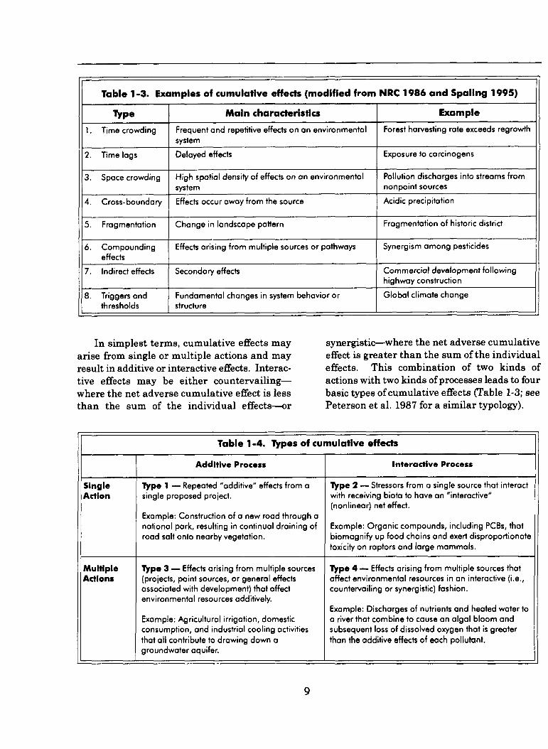
Table 1-3. Examples of cumulative effects (modified from NRC 1986 and Spaling 1995)

Type Main characteristics Example

1. Time crowding Frequent and repetitive effects on an environmental Forest harvesting rate exceeds regrowth

system

2. Time lags Delayed effects Exposure to carcinogens

3. Space crowding High spatial density of effects on on environmental Pollution discharges inta streams from

system nonpoint sources

4. Cross-boundary Effects occur away from the source Acidic precipitation

5. Fragmentation Change in landscape pattern Fragmentation of historic district

6. Compounding Effects arising from multiple sources ar pathways Synergism among pesticides

effects

7. Indirect effects Secondary effects Commercial development following

highway construction

8. Triggers and Fundamental changes in system behavior or Global climate change

thresholds structure

In simplest terms, cumulative effects may synergistic-where the net adverse cumulativearise from single or multiple actions and may effect is greater than the sum of the individualresult in additive or interactive effects. Interac- effects. This combination of two kinds oftive effects may be either countervailing— actions with two kinds of processes leads to fourwhere the net adverse cumulative effect is Iess basic types of cumulative effects (Table 1-3; seethan the sum of the individual effects-r Peterson et al. 1987 for a similar typology).

51ngleMien

MultipieActions

Tabie 1-4. ~pes of cumulative effects

Additive Process

Type 1 — Repeated “additive” effects from a

single proposed proiect.

Example: Construction of a new road through a

national park, resulting in continual draining of

road salt onto nearby vegetation.

Type 3 – Effects arising from multiple sources

(proiects, point sources, or general effects

associated with development) that affect

environmental resources additively.

Example: Agricultural irrigation, domestic

consumption, and industrial cooling activities

that all contribute to drawing down a

groundwater aquifer.

Interactive Process

Qpe 2 - Stressors from a single source that interact

with receiving biota to have an “interactive”

(nonlinear) net effect.

Example: Organic compounds, including PCBS, that

biomagnify up food chains and exert disproportionate

toxicity on raptors and large mammals.

Type 4- Effects arising fram multiple sources that

affect environmental resources in an interactive (i.e.,

countervailing or synergistic) fashion.

Example: Discharges of nutrients and heated water to

a river that combine to cause an algal bloom and

subsequent loss of dissolved oxygen that is greater

than the additive effects of each pollutant.

9

ROADMAP TO THE HANDBOOK to be accomplished can be identfied in eachcomponent of the NEPA process; each chapter

The chapters that follow discuss the focuses on its constituent steps (Table 1-4). Theincorporation of cumulative effects analysis into last chapter of this report discusses developingthe components of environmental impact a cumulative effects analysis methodology thatassessment: scoping (Chapter 2), describing the draws upon existing methods, techniques, andaffected environment (Chapter 3), and deter- tools to analyze cumulative effects. Appendix Amining the environmental consequences provides brief descriptions of 11 cumulative(Chapter 4). Although cumulative effects anal- effects analysis methods.ysis is an iterative process, basic steps that

Table 1-5. Steps in cumulative effects analysis (CEA) to be addressed in each component ofenvironmental impact assessment (EIA)

EIA Components CEA Steps

Scoping 1. Identify the significant cumulative effects issues associated with the

proposed action and define the assessment goals.

2. Establish the geographic scope for the analysis.

3. Establish the time frame for the analysis.

4. Identify other actions affecting the resources, ecosystems, and

human communities of concern.

Describing the Affected 5. Characterize the resources, ecosystems, and human communities

Environment identified in scoping in terms of their response to change and

capacity to withstand stresses.

6, Characterize the stresses affecting these resources, ecosystems, and

human communities and their relation to regulatory thresholds,

7. Define a baseline condition for the resources, ecosystems, and

human communities.

Determining the Environmental 8. Identify the important cause-and-effect relationships between human

Consequences activities and resources, ecosystems, and human communities.

9. Determine the mognitude and significance of cumulative effects.

10. Modify or add alternatives to avoid, minimize, or mitigate significant

cumulative effects.

11. Monitor the cumulative effects of the selected alternative and adapt

management.

10

11

PRINCIPLES

• Include past, present, and future actions.

• Include all federal, nonfederal, and privateactions.

• Focus on each affected resource,ecosystem, and human community.

• Focus on truly meaningful effects.

Step 1

Step 2

Step 3

Step 4

([SDQGLQJ HQYLURQPHQWDO LPSDFW DVVHVV�PHQW WR LQFRUSRUDWH FXPXODWLYH HIIHFWV FDQ RQO\EH DFFRPSOLVKHG E\ WKH HQOLJKWHQHG XVH RI WKHVFRSLQJ SURFHVV� 7KH SXUSRVH RI VFRSLQJ IRUFXPXODWLYH HIIHFWV LV WR GHWHUPLQH �� ZKHWKHUWKH UHVRXUFHV� HFRV\VWHPV� DQG KXPDQFRPPXQLWLHV RI FRQFHUQ KDYH DOUHDG\ EHHQDIIHFWHG E\ SDVW RU SUHVHQW DFWLYLWLHV DQG ��ZKHWKHU RWKHU DJHQFLHV RU WKH SXEOLF KDYH SODQVWKDW PD\ DIIHFW WKH UHVRXUFHV LQ WKH IXWXUH� 7KLVLV EHVW DFFRPSOLVKHG DV DQ LWHUDWLYH SURFHVV� RQHWKDW JRHV EH\RQG IRUPDO VFRSLQJ PHHWLQJV DQGFRQVXOWDWLRQV WR LQFOXGH FUHDWLYH LQWHUDFWLRQVZLWK DOO WKH VWDNHKROGHUV� 6FRSLQJ VKRXOG EHXVHG LQ ERWK WKH SODQQLQJ DQG SURMHFWGHYHORSPHQW VWDJH �L�H�� ZKHQHYHU LQIRUPDWLRQRQ FXPXODWLYH HIIHFWV ZLOO FRQWULEXWH WR D EHWWHUGHFLVLRQ��

6FRSLQJ LQIRUPDWLRQ PD\ FRPH IURPDJHQF\ FRQVXOWDWLRQV� SXEOLF FRPPHQWV� WKHDQDO\VWV RZQ NQRZOHGJH DQG H[SHULHQFH�SODQQLQJ DFWLYLWLHV� WKH SURSRQHQWV VWDWHPHQWVRI SXUSRVH DQG QHHG� XQGHUO\LQJ VWXGLHV LQVXSSRUW RI WKH SURMHFW SURSRVDO� H[SHUW RSLQLRQ�

RU RWKHU 1(3$ DQDO\VHV� 7KLV LQIRUPDWLRQ VXS�SRUWV DOO WKH VWHSV LQ FXPXODWLYH HIIHFWV DQDO\VLV�LQFOXGLQJ LGHQWLI\LQJ GDWD IRU HVWDEOLVKLQJ WKHHQYLURQPHQWDO EDVHOLQH �VHH &KDSWHU �� DQGLGHQWLI\LQJ LQIRUPDWLRQ UHODWHG WR LPSDFWVLJQLILFDQFH �VHH &KDSWHU �� 0RVW LPSRUWDQWO\�KRZHYHU� VFRSLQJ IRU FXPXODWLYH HIIHFWV VKRXOGLQFOXGH WKH IROORZLQJ VWHSV�

Identify the significant cumulativeeffects issues associated with theproposed action and define theassessment goals.

Establish the geographic scopefor the analysis.

Establish the time frame for theanalysis.

Identify other actions affectingthe resources, ecosystems, andhuman communities of concern.

IDENTIFYING CUMULATIVE EFFECTS ISSUES

,GHQWLI\LQJ WKH PDMRU FXPXODWLYH HIIHFWVLVVXHV RI D SURMHFW LQYROYHV GHILQLQJ WKH IROORZ�LQJ�

P WKH GLUHFW DQG LQGLUHFW HIIHFWV RI WKHSURSRVHG DFWLRQ�

P ZKLFK UHVRXUFHV� HFRV\VWHPV� DQG KX�PDQ FRPPXQLWLHV� DUH DIIHFWHG� DQG

P ZKLFK HIIHFWV RQ WKHVH UHVRXUFHV DUHLPSRUWDQW IURP D FXPXODWLYH HIIHFWVSHUVSHFWLYH�

12

7KH SURSRVHG DFWLRQ PD\ DIIHFW VHYHUDO UH� DV ZHOO DV WKH UHJLRQDO KLVWRU\ RI FXPXODWLYHVRXUFHV HLWKHU GLUHFWO\ RU LQGLUHFWO\� 5HVRXUFHV ZHWODQG ORVVHV DQG GHJUDGDWLRQ� DQG WKHFDQ EH HOHPHQWV RI WKH SK\VLFDO HQYLURQPHQW� SUHVHQFH RI RWKHU SURSRVDOV WKDW ZRXOG SURGXFHVSHFLHV� KDELWDWV� HFRV\VWHP SDUDPHWHUV DQG IXWXUH ZHWODQG ORVVHV RU GHJUDGDWLRQ�IXQFWLRQV� FXOWXUDO UHVRXUFHV� UHFUHDWLRQDO RSSRU�WXQLWLHV� KXPDQ FRPPXQLW\ VWUXFWXUH� WUDIILFSDWWHUQV� RU RWKHU HFRQRPLF DQG VRFLDOFRQGLWLRQV� ,Q D EURDG VHQVH� DOO WKH LPSDFWV RQDIIHFWHG UHVRXUFHV DUH SUREDEO\ FXPXODWLYH�KRZHYHU� WKH UROH RI WKH DQDO\VW LV WR QDUURZ WKHIRFXV RI WKH FXPXODWLYH HIIHFWV DQDO\VLV WRLPSRUWDQW LVVXHV RI QDWLRQDO� UHJLRQDO� RU ORFDOVLJQLILFDQFH� 7KLV QDUURZLQJ FDQ RFFXU RQO\DIWHU WKRURXJK VFRSLQJ� 7KH DQDO\VW VKRXOG DVNEDVLF TXHVWLRQV VXFK DV ZKHWKHU WKH SURSRVHGDFWLRQ ZLOO KDYH HIIHFWV VLPLODU WR RWKHU DFWLRQVLQ WKH DUHD DQG ZKHWKHU WKH UHVRXUFHV KDYH EHHQKLVWRULFDOO\ DIIHFWHG E\ FXPXODWLYH DFWLRQV�7DEOH �� 0DQ\ VLJQLILFDQW FXPXODWLYH HIIHFWVLVVXHV DUH ZHOO NQRZQ� 3XEOLF LQWHUHVW JURXSV�QDWXUDO UHVRXUFH DQG ODQG PDQDJHPHQW DJHQF�LHV� DQG UHJXODWRU\ DJHQFLHV UHJXODUO\ GHDO ZLWKFXPXODWLYH HIIHFWV� 1HZVSDSHUV DQG VFLHQWLILFMRXUQDOV IUHTXHQWO\ SXEOLVK OHWWHUV DQG FRP�PHQWV GHDOLQJ ZLWK WKHVH LVVXHV�

1RW DOO SRWHQWLDO FXPXODWLYH HIIHFWV LVVXHVLGHQWLILHG GXULQJ VFRSLQJ QHHG WR EH LQFOXGHG LQDQ ($ RU DQ (,6� 6RPH PD\ EH LUUHOHYDQW RULQFRQVHTXHQWLDO WR GHFLVLRQV DERXW WKH SURSRVHGDFWLRQ DQG DOWHUQDWLYHV� &XPXODWLYH HIIHFWVDQDO\VLV VKRXOG �FRXQW ZKDW FRXQWV�� QRW SUR�GXFH VXSHUILFLDO DQDO\VHV RI D ORQJ ODXQGU\ OLVW RILVVXHV WKDW KDYH OLWWOH UHOHYDQFH WR WKH HIIHFWV RIWKH SURSRVHG DFWLRQ RU WKH HYHQWXDO GHFLVLRQV�%HFDXVH FXPXODWLYH HIIHFWV FDQ UHVXOW IURP WKHDFWLYLWLHV RI RWKHU DJHQFLHV RU SHUVRQV� WKH\ PD\KDYH DOUHDG\ EHHQ DQDO\]HG E\ RWKHUV DQG WKHLPSRUWDQFH RI WKH LVVXH GHWHUPLQHG� )RU LQ�VWDQFH� DQ DJHQF\ SURSRVLQJ DQ DFWLRQ ZLWKPLQRU HIIHFWV RQ ZHWODQGV VKRXOG QRW XQL�ODWHUDOO\ GHFLGH WKDW FXPXODWLYH HIIHFWV RQZHWODQGV LV QRW DQ LPSRUWDQW LVVXH� &XPXODWLYHHIIHFWV DQDO\VLV VKRXOG FRQVLGHU WKH FRQFHUQV RIDJHQFLHV PDQDJLQJ DQG UHJXODWLQJ ZHWODQGV�

BOUNDING CUMULATIVE EFFECTSANALYSIS

2QFH WKH VWXG\ JRDOV RI WKH FXPXODWLYHHIIHFWV DQDO\VLV DUH HVWDEOLVKHG� WKH DQDO\VWPXVW GHFLGH RQ WKH VSHFLILF FRQWHQW RI WKH VWXG\WKDW ZLOO PHHW WKRVH UHTXLUHPHQWV� $QDO\]LQJFXPXODWLYH HIIHFWV GLIIHUV IURP WKH WUDGLWLRQDODSSURDFK WR HQYLURQPHQWDO LPSDFW DVVHVVPHQWEHFDXVH LW UHTXLUHV WKH DQDO\VW WR H[SDQG WKHJHRJUDSKLF ERXQGDULHV DQG H[WHQG WKH WLPHIUDPH WR HQFRPSDVV DGGLWLRQDO HIIHFWV RQ WKHUHVRXUFHV� HFRV\VWHPV� DQG KXPDQ FRPPXQLWLHVRI FRQFHUQ�

Identifying Geographic Boundaries

)RU D SURMHFW�VSHFLILF DQDO\VLV� LW LV RIWHQVXIILFLHQW WR DQDO\]H HIIHFWV ZLWKLQ WKH LPPH�GLDWH DUHD RI WKH SURSRVHG DFWLRQ� :KHQ DQD�O\]LQJ WKH FRQWULEXWLRQ RI WKLV SURSRVHG DFWLRQ WRFXPXODWLYH HIIHFWV� KRZHYHU� WKH JHRJUDSKLFERXQGDULHV RI WKH DQDO\VLV DOPRVW DOZD\V VKRXOGEH H[SDQGHG� 7KHVH H[SDQGHG ERXQGDULHV FDQEH WKRXJKW RI DV GLIIHUHQFHV LQ KLHUDUFK\ RUVFDOH� 3URMHFW�VSHFLILF DQDO\VHV DUH XVXDOO\FRQGXFWHG RQ WKH VFDOH RI FRXQWLHV� IRUHVW PDQ�DJHPHQW XQLWV� RU LQVWDOODWLRQ ERXQGDULHV�ZKHUHDV FXPXODWLYH HIIHFWV DQDO\VLV VKRXOG EHFRQGXFWHG RQ WKH VFDOH RI KXPDQ FRPPXQLWLHV�ODQGVFDSHV� ZDWHUVKHGV� RU DLUVKHGV� &KRRVLQJWKH DSSURSULDWH VFDOH WR XVH LV FULWLFDO DQG ZLOOGHSHQG RQ WKH UHVRXUFH RU V\VWHP� )LJXUH ��LOOXVWUDWHV WKH XWLOLW\ RI XVLQJ WKH HFRORJLFDOO\UHOHYDQW ZDWHUVKHG ERXQGDU\ RI WKH $QDFRVWLD5LYHU EDVLQ UDWKHU WKDQ WKH SROLWLFDO ERXQGDULHVRI ORFDO JRYHUQPHQWV WR GHYHORS UHVWRUDWLRQSODQV�

$ XVHIXO FRQFHSW LQ GHWHUPLQLQJ DSSURSULDWHJHRJUDSKLF ERXQGDULHV IRU D FXPXODWLYH HIIHFWVDQDO\VLV LV WKH SURMHFW LPSDFW ]RQH�

13

Table 2-1. Identifying potential cumulative effects issues related to a proposed action

1. What is the value of the affected resource or ecosystem? Is it:

P protected by legislation or planning goals?P ecologically important?P culturally important?P economically important?P important to the well-being of a human community?

2. Is the proposed action one of several similar past, present, or future actions in the same geographic area?(Regions may be land management units, watersheds, regulatory regions, states, ecoregions, etc.) Examples:timber sales in a national forest; hydropower development on a river; incinerators in a community.

3. Do other activities (whether governmental or private) in the region have environmental effects similar to those ofthe proposed action? Example: release of oxidizing pollutants to a river by a municipality, an industry, orindividual septic systems.

4. Will the proposed action (in combination with other planned activities) affect any natural resources; culturalresources; social or economic units; or ecosystems of regional, national, or global public concern? Examples:release of chlorofluorocarbons to the atmosphere; conversion of wetland habitat to farmland located in a migratorywaterfowl flyway.

5. Have any recent or ongoing NEPA analyses of similar actions or nearby actions identified important adverse orbeneficial cumulative effect issues? Examples: National Forest Plan EIS; Federal Energy Regulatory CommissionBasinwide EIS or EA.

6. Has the impact been historically significant, such that the importance of the resource is defined by past loss, pastgain, or investments to restore resources? Example: mudflat and salt-marsh habitats in San Francisco Bay.

7. Might the proposed action involve any of the following cumulative effects issues?

P long range transport of air pollutants resulting in ecosystem acidification or eutrophicationP air emissions resulting in degradation of regional air qualityP release of greenhouse gases resulting in climate modificationP loading large water bodies with discharges of sediment, thermal, and toxic pollutantsP reduction or contamination of groundwater suppliesP changes in hydrological regimes of major rivers and estuariesP long-term containment and disposal of hazardous wastesP mobilization of persistent or bioaccumulated substances through the food chainP decreases in the quantity and quality of soilsP loss of natural habitats or historic character through residential, commercial, and industrial developmentP social, economic, or cultural effects on low-income or minority communities resulting from ongoing

developmentP habitat fragmentation from infrastructure construction or changes in land useP habitat degradation from grazing, timber harvesting, and other consumptive usesP disruption of migrating fish and wildlife populationsP loss of biological diversity

14Figure 2-1. Juxtaposition of natural and political boundaries surrounding the Anacostia River

15

)RU D SURSRVHG DFWLRQ RU UHDVRQDEOH DOWHUQDWLYH� 3URMHFW LPSDFW ]RQHV IRU D SURSRVHG DFWLRQWKH DQDO\VWV VKRXOG

P 'HWHUPLQH WKH DUHD WKDW ZLOO EH DIIHFWHGE\ WKDW DFWLRQ� 7KDW DUHD LV WKH SURMHFWLPSDFW ]RQH�

P 0DNH D OLVW RI WKH UHVRXUFHV ZLWKLQ WKDW]RQH WKDW FRXOG EH DIIHFWHG E\ WKH SUR�SRVHG DFWLRQ�

P 'HWHUPLQH WKH JHRJUDSKLF DUHDV RFFXSLHGE\ WKRVH UHVRXUFHV RXWVLGH RI WKH SURMHFWLPSDFW ]RQH� ,Q PRVW FDVHV� WKH ODUJHVW RIWKHVH DUHDV ZLOO EH WKH DSSURSULDWH DUHDIRU WKH DQDO\VLV RI FXPXODWLYH HIIHFWV�

P 'HWHUPLQH WKH DIIHFWHG LQVWLWXWLRQDO MXULV�GLFWLRQV� ERWK IRU WKH SURSRVLQJ DJHQF\DQG RWKHU DJHQFLHV RU JURXSV�

DUH OLNHO\ WR YDU\ IRU GLIIHUHQW UHVRXUFHV DQGHQYLURQPHQWDO PHGLD� )RU ZDWHU� WKH SURMHFWLPSDFW ]RQH ZRXOG EH OLPLWHG WR WKH K\GURORJLFV\VWHP WKDW ZRXOG EH DIIHFWHG E\ WKH SURSRVHGDFWLRQ� )RU DLU� WKH ]RQH PD\ EH WKH SK\VLR�JUDSKLF EDVLQ LQ ZKLFK WKH SURSRVHG DFWLRQZRXOG EH ORFDWHG� /DQG�EDVHG HIIHFWV PD\ RFFXUZLWKLQ VRPH VHW GLVWDQFH IURP WKH SURSRVHGDFWLRQ� ,Q DGGLWLRQ� WKH ERXQGDULHV IRU DQ LQGL�YLGXDO UHVRXUFH VKRXOG EH UHODWHG WR WKHUHVRXUFHV GHSHQGHQFH RQ GLIIHUHQW HQYLURQ�PHQWDO PHGLD� 7DEOH �� SURYLGHV VRPH SRVVLEOHJHRJUDSKLF ERXQGDULHV IRU GLIIHUHQW UHVRXUFHV�7KLV OLVW LV QRW LQFOXVLYH� 7KH DSSOLFDEOH JHR�JUDSKLF VFRSH QHHGV WR EH GHILQHG FDVH E\ FDVH�

Table 2-2. Geographic areas that could be used in a cumulative effects analysis

Resource Possible Geographic Areas for Analysis

Air quality Metropolitan area, airshed, or global atmosphere

Water quality Stream, watershed, river basin, estuary, aquifer, or parts thereof

Vegetative Watershed, forest, range, or ecosystemresources

Resident wildlife Species habitat or ecosystem

Migratory wildlife Breeding grounds, migration route, wintering areas, or total range of affected population units

Fishery resources Stream, river basin, estuary, or parts thereof; spawning area and migration route

Historic resources Neighborhood, rural community, city, state, tribal territory, known or possible historic district

Sociocultural Neighborhood, community, distribution of low-income or minority population, or culturallyresources valued landscape

Land use Community, metropolitan area, county, state, or region

Coastal zone Coastal region or watershed

Recreation River, lake, geographic area, or land management unit

Socioeconomics Community, metropolitan area, county, state, or country

16

2QH ZD\ WR HYDOXDWH JHRJUDSKLF ERXQGDULHV WKH FXPXODWLYH HIIHFWV DQDO\VLV� 7KH DQDO\VWLV WR FRQVLGHU WKH GLVWDQFH DQ HIIHFW FDQ WUDYHO� VKRXOG DWWHPSW WR LGHQWLI\ DFWLRQV WKDW FRXOG)RU LQVWDQFH� DLU HPLVVLRQV FDQ WUDYHO VXE� UHDVRQDEO\ EH H[SHFWHG WR RFFXU ZLWKLQ WKDWVWDQWLDO GLVWDQFHV DQG DUH DQ LPSRUWDQW SDUW RI SHULRG�UHJLRQDO DLU TXDOLW\� $LU TXDOLW\ UHJLRQV DUHGHILQHG E\ WKH (3$� DQG WKHVH UHJLRQV DUH DQDSSURSULDWH ERXQGDU\ IRU DVVHVVPHQW RI WKHFXPXODWLYH HIIHFWV RI UHOHDVHV RI SROOXWDQWV WR WKHDWPRVSKHUH� )RU ZDWHU UHVRXUFHV� DQ DSSUR�SULDWH UHJLRQDO ERXQGDU\ PD\ EH D ULYHU EDVLQ RUSDUWV WKHUHRI� :DWHUVKHG ERXQGDULHV DUH XVHIXOIRU FXPXODWLYH HIIHFWV DQDO\VLV EHFDXVH �� SRO�OXWDQWV DQG PDWHULDO UHOHDVHG LQ WKH ZDWHUVKHGPD\ WUDYHO GRZQVWUHDP WR EH PLQJOHG ZLWK RWKHUSROOXWDQWV DQGPDWHULDOV� �� PLJUDWRU\ ILVK PD\WUDYHO XS DQG GRZQ WKH ULYHU V\VWHP GXULQJWKHLU OLIH F\FOH� DQG �� UHVRXUFH DJHQFLHV PD\KDYH EDVLQ�ZLGH PDQDJHPHQW DQG SODQQLQJJRDOV� )RU ODQG�EDVHG HIIHFWV� DQ DSSURSULDWHUHJLRQDO ERXQGDU\ PD\ EH D �IRUHVW RU UDQJH�� DZDWHUVKHG� DQ HFRORJLFDO UHJLRQ �HFRUHJLRQ�� RUVRFLRHFRQRPLF UHJLRQ �IRU HYDOXDWLQJ HIIHFWV RQKXPDQ FRPPXQLWLHV�� :KLFK ERXQGDU\ LV WKHPRVW DSSURSULDWH GHSHQGV ERWK RQ WKH DFFXPX�ODWLRQ FKDUDFWHULVWLFV RI WKH HIIHFWV EHLQJDVVHVVHG DQG DQ HYDOXDWLRQ RI WKH PDQDJHPHQWRU UHJXODWRU\ LQWHUHVWV RI WKH DJHQFLHV LQYROYHG�

Identifying Time Frames

7KH WLPH IUDPH RI WKH SURMHFW�VSHFLILF DQDO\�VLV VKRXOG DOVR EH HYDOXDWHG WR GHWHUPLQH LWVDSSOLFDELOLW\ WR WKH FXPXODWLYH HIIHFWV DQDO\VLV�7KLV DVSHFW RI WKH FXPXODWLYH HIIHFWV DQDO\VLVPD\ DW ILUVW VHHP WKH PRVW WURXEOHVRPH WRGHILQH� &(4ªV UHJXODWLRQV GHILQH FXPXODWLYHHIIHFWV DV WKH §LQFUHPHQWDO HIIHFW RI WKH DFWLRQZKHQ DGGHG WR RWKHU SDVW� SUHVHQW� DQG UHDVRQ�DEO\ IRUHVHHDEOH IXWXUH DFWLRQV� �� &)5 �� ,Q GHWHUPLQLQJ KRZ IDU LQWR WKH IXWXUHWR DQDO\]H FXPXODWLYH HIIHFWV� WKH DQDO\VW VKRXOGILUVW FRQVLGHU WKH WLPH IUDPH RI WKH SURMHFW�VSHFLILF DQDO\VLV� ,I WKH HIIHFWV RI WKH SURSRVHGDFWLRQ DUH SURMHFWHG WR ODVW ILYH \HDUV� WKLV WLPHIUDPH PD\ EH WKH PRVW DSSURSULDWH IRU

7KHUH PD\ EH LQVWDQFHV ZKHQ WKH WLPH IUDPHRI WKH SURMHFW�VSHFLILF DQDO\VLV ZLOO QHHG WR EHH[SDQGHG WR HQFRPSDVV FXPXODWLYH HIIHFWVRFFXUULQJ IXUWKHU LQWR WKH IXWXUH �)LJXUH ��)RU LQVWDQFH� HYHQ WKRXJK WKH HIIHFWV RI DSURSRVHG DFWLRQ PD\ OLQJHU RU GHFUHDVH VORZO\WKURXJK WLPH� WKH WLPH IUDPH IRU WKH SURMHFW�VSHFLILF DQDO\VLV XVXDOO\ GRHV QRW H[WHQG EH\RQGWKH WLPH ZKHQ SURMHFW�VSHFLILF HIIHFWV GURS EHORZD OHYHO GHWHUPLQHG WR EH VLJQLILFDQW� 7KHVHSURMHFW�VSHFLILF HIIHFWV� KRZHYHU� PD\ FRPELQHZLWK WKH HIIHFWV RI RWKHU DFWLRQV EH\RQG WKH WLPHIUDPH RI WKH SURSRVHG DFWLRQ DQG UHVXOW LQ VLJ�QLILFDQW FXPXODWLYH HIIHFWV WKDW PXVW EH FRQ�VLGHUHG�

IDENTIFYING PAST, PRESENT, ANDREASONABLY FORESEEABLE FUTUREACTIONS

$V GHVFULEHG DERYH� LGHQWLI\LQJ SDVW� SUHV�HQW� DQG IXWXUH DFWLRQV LV FULWLFDO WR HVWDEOLVKLQJWKH DSSURSULDWH JHRJUDSKLF DQG WLPH ERXQGDULHVIRU WKH FXPXODWLYH HIIHFWV DQDO\VLV� ,GHQWLI\LQJERXQGDULHV DQG DFWLRQV VKRXOG EH LWHUDWLYHZLWKLQ WKH VFRSLQJ SURFHVV�

$ VFKHPDWLF GLDJUDP VKRZLQJ WKH DUHD LQZKLFK WKH SURSRVHG DFWLRQ LV ORFDWHG� WKH ORFD�WLRQ RI UHVRXUFHV� DQG WKH ORFDWLRQ RI RWKHUIDFLOLWLHV �H[LVWLQJ RU SODQQHG�� KXPDQ FRP�PXQLWLHV� DQG GLVWXUEHG DUHDV FDQ EH XVHIXO IRULGHQWLI\LQJ DFWLRQV WR EH LQFOXGHG LQ WKH FXP�XODWLYH HIIHFWV DQDO\VLV �)LJXUH �� $ JHR�JUDSKLF LQIRUPDWLRQ V\VWHP �*,6� RU D PDQXDOPDS RYHUOD\ V\VWHP FDQ EH XVHG WR GHSLFW WKLVLQIRUPDWLRQ �VHH $SSHQGL[ $ IRU D GHVFULSWLRQ RIPDS RYHUOD\V DQG *,6�� 6XFK D GLDJUDP LV LVXVHIXO IRU GHWHUPLQLQJ SURMHFW�VSHFLILF LPSDFW]RQHV DQG WKHLU RYHUODS ZLWK DUHDV DIIHFWHG E\RWKHU QRQSURMHFW DFWLRQV�

17

Figure 2-2. Time frames for project-specific and cumulative effects analyses

%\ H[DPLQLQJ WKH RYHUODS RI LPSDFW ]RQHV RQ WKHLU LPSDFW ]RQHV RYHUODS DUHDV RFFXSLHG E\WKH DUHDV RFFXSLHG E\ UHVRXUFHV� LW VKRXOG EH UHVRXUFHV DIIHFWHG E\ WKH SURSRVHG DFWLRQ�SRVVLEOH WR UHILQH WKH OLVW RI SURMHFWV RU DFWLYLWLHV�SDVW� SUHVHQW� RU IXWXUH� WR EH LQFOXGHG LQ WKHDQDO\VLV� 3UR[LPLW\ RI DFWLRQV PD\ QRW EHVXIILFLHQW MXVWLILFDWLRQ WR LQFOXGH WKHP LQ WKHDQDO\VLV� ,Q WKH H[DPSOH VKRZQ LQ )LJXUH ��WKH FXPXODWLYH HIIHFWV DQDO\VLV IRU WURXW VKRXOGFRQVLGHU WKH HIIHFWV RI WKH H[LVWLQJ PLQH DQG WKHSODQQHG ORJJLQJ DFWLYLW\� EHFDXVH WKHVH DFWLYLWLHVZRXOG KDYH HLWKHU SUHVHQW RU IXWXUH HIIHFWV RQWKH WURXW VSDZQLQJ DUHD EHORZ WKH SURSRVHGSRZHU SODQW IDFLOLW\� $OWKRXJK DQ DJULFXOWXUDODUHD LV QHDUE\� LW FDQ EH H[FOXGHG IURP WKHDQDO\VLV EHFDXVH LWV VHGLPHQW ORDGLQJ HIIHFWVRFFXU GRZQVWUHDP RI WKH WURXW VSDZQLQJ DUHD�3UR[LPLW\ RI RWKHU DFWLRQV WR WKH SURSRVHG DFWLRQ 7KH DYDLODELOLW\ RI GDWD RIWHQ GHWHUPLQHVLV QRW WKH GHFLVLYH IDFWRU IRU LQFOXGLQJ WKHVH KRZ IDU EDFN SDVW HIIHFWV DUH H[DPLQHG�DFWLRQV LQ DQ DQDO\VLV� WKHVH DFWLRQV PXVW KDYH $OWKRXJK FHUWDLQ W\SHV RI GDWD �H�J�� IRUHVW FRYHU�VRPH LQIOXHQFH RQ WKH UHVRXUFHV DIIHFWHG E\ WKH PD\ EH DYDLODEOH IRU H[WHQVLYH SHULRGV LQ WKHSURSRVHG DFWLRQ� ,Q RWKHU ZRUGV� WKHVH RWKHU SDVW �L�H�� VHYHUDO GHFDGHV�� RWKHU GDWD �H�J��DFWLRQV VKRXOG EH LQFOXGHG LQ DQDO\VLV ZKHQ ZDWHU TXDOLW\ GDWD� PD\ EH DYDLODEOH RQO\ IRU

&RPSOHWLQJ WKH JHRJUDSKLF RU VFKHPDWLF GLD�JUDP GHSHQGLQJ RQ DSSO\LQJ FDXVH�DQG�HIIHFWPRGHOV WKDW OLQN KXPDQ DFWLRQV DQG WKH UH�VRXUFHV RU HFRV\VWHPV� 7KLV WRR LV DQ LWHUDWLYHSURFHVV� ,GHQWLI\LQJ RWKHU DFWLYLWLHV FRQWULEXW�LQJ WR FXPXODWLYH HIIHFWV FRXOG UHVXOW LQ WKHDGGLWLRQ RI QHZ HIIHFW SDWKZD\V WR WKH FDXVH�DQG�HIIHFW PRGHO� ,Q WKH H[DPSOH� DGGLWLRQ RI DQH[LVWLQJ PLQH WR WKH FXPXODWLYH HIIHFWV DQDO\VLVFRXOG UHTXLUH DGGLQJ D SDWKZD\ IRU WKH HIIHFWV RIFKHPLFDO SROOXWLRQ RQ WURXW� &KDSWHUV � DQG �DQG $SSHQGL[ $ GLVFXVV FDXVH�DQG�HIIHFW PRGHO�LQJ DQG QHWZRUN DQDO\VLV�

18Figure 2-3. Impact zones of proposed and existing development relative to a trout population

19

PXFK VKRUWHU SHULRGV� %HFDXVH WKH GDWD GHVFULE� IRUHVHHDEOH DFWLRQV E\ SULYDWH RUJDQL]DWLRQV RULQJ SDVW FRQGLWLRQV DUH XVXDOO\ VFDUFH� WKH DQDO� LQGLYLGXDOV DUH XVXDOO\ PRUH GLIILFXOW WR LGHQWLI\\VLV RI SDVW HIIHFWV LV RIWHQ TXDOLWDWLYH� WKDQ WKRVH RI IHGHUDO RU RWKHU JRYHUQPHQWDO

,GHQWLI\LQJ VLPLODU DFWLRQV SUHVHQWO\ XQGHU�ZD\ LV HDVLHU WKDQ LGHQWLI\LQJ SDVW RU IXWXUHDFWLRQV� EXW LW LV E\ QR PHDQV VLPSOH� %HFDXVHPRVW RI WKH DQDO\WLFDO HIIRUW LQ DQ HQYLURQPHQWDOLPSDFW DVVHVVPHQW GHDOV ZLWK WKH SURSRVHGDFWLRQ� WKH DFWLRQV RI RWKHU DJHQFLHV DQG SULYDWHSDUWLHV DUH XVXDOO\ OHVV ZHOO NQRZQ� (IIHFWLYHFXPXODWLYH HIIHFWV DQDO\VLV UHTXLUHV FORVHFRRUGLQDWLRQ DPRQJ DJHQFLHV WR HQVXUH WKDW HYHQDOO SUHVHQW DFWLRQV� PXFK OHVV SDVW DQG IXWXUHDFWLRQV� DUH FRQVLGHUHG�

7KH ILUVW VWHS LQ LGHQWLI\LQJ IXWXUH DFWLRQV LV EXW LW LV LPSRUWDQW WR LQGLFDWH LQ WKH 1(3$WR LQYHVWLJDWH WKH SODQV RI WKH SURSRQHQW DJHQF\ DQDO\VLV ZKHWKHU WKHVH SODQV ZHUH SUHVHQWHG E\DQG RWKHU DJHQFLHV LQ WKH DUHD� &RPPRQO\� WKH SULYDWH SDUW\ UHVSRQVLEOH IRU RULJLQDWLQJ WKHDQDO\VWV RQO\ LQFOXGH WKRVH SODQV IRU DFWLRQV DFWLRQ� :KHQHYHU VSHFXODWLYH SURMHFWLRQV RIZKLFK DUH IXQGHG RU IRU ZKLFK RWKHU 1(3$ IXWXUH GHYHORSPHQW DUH XVHG� WKH DQDO\VW VKRXOGDQDO\VLV LV EHLQJ SUHSDUHG� 7KLV DSSURDFK GRHV SURYLGH DQ H[SOLFLW GHVFULSWLRQ RI WKHQRW PHHW WKH OHWWHU RU LQWHQW RI &(4ªV UHJXOD� DVVXPSWLRQV LQYROYHG� ,I WKH DQDO\VW LV XQFHU�WLRQV� ,W XQGHUHVWLPDWHV WKH QXPEHU RI IXWXUH WDLQ ZKHWKHU WR LQFOXGH IXWXUH DFWLRQV� LW PD\ EHSURMHFWV� EHFDXVH PDQ\ YLDEOH DFWLRQV PD\ EH LQ DSSURSULDWH WR ERXQG WKH SUREOHP E\ GHYHORSLQJWKH HDUO\ SODQQLQJ VWDJH� 2Q WKH RWKHU KDQG� VHYHUDO VFHQDULRV ZLWK GLIIHUHQW DVVXPSWLRQVVRPH DFWLRQV LQ WKH SODQQLQJ� EXGJHWLQJ� RU DERXW IXWXUH DFWLRQV�H[HFXWLRQ SKDVH PD\ QRW JR IRUZDUG� 7R LQFOXGHDOO SURSRVDOV HYHU FRQVLGHUHG DV RWKHU DFWLRQVZRXOG PRVW OLNHO\ RYHUHVWLPDWH WKH IXWXUHHIIHFWV RI FXPXODWLYH HIIHFWV RQ WKH UHVRXUFHV� P WKH DFWLRQ LV RXWVLGH WKH JHRJUDSKLFHFRV\VWHPV� DQG KXPDQ FRPPXQLWLHV� WKHUHIRUH�WKH DQDO\VW VKRXOG GHYHORS JXLGHOLQHV DV WRZKDW FRQVWLWXWHV �UHDVRQDEO\ IRUHVHHDEOH IXWXUHDFWLRQV� EDVHG RQ WKH SODQQLQJ SURFHVV ZLWKLQHDFK DJHQF\� 6SHFLILFDOO\� WKH DQDO\VW VKRXOGXVH WKH EHVW DYDLODEOH LQIRUPDWLRQ WR GHYHORSVFHQDULRV WKDW SUHGLFW ZKLFK IXWXUH DFWLRQVPLJKW UHDVRQDEO\ EH H[SHFWHG DV D UHVXOW RI WKHSURSRVDO� 6XFK VFHQDULRV DUH JHQHUDOO\ EDVHG RQH[SHULHQFH REWDLQHG IURP VLPLODU SURMHFWV OR�FDWHG HOVHZKHUH LQ WKH UHJLRQ� ,QFOXGLQJ IXWXUHDFWLRQV LQ WKH VWXG\ LV PXFK HDVLHU LI DQ DJHQF\KDV DOUHDG\ GHYHORSHG D SODQQLQJ GRFXPHQW WKDWLGHQWLILHV SURSRVHG IXWXUH DFWLRQV DQG KDV FRP�PXWLODWHG WKHVH SODQV WR RWKHU IHGHUDO DJHQFLHVDQG JRYHUQPHQWDO ERGLHV LQ WKH DIIHFWHG UHJLRQ�

:KHQ LGHQWLI\LQJ IXWXUH DFWLRQV WR LQFOXGH LQWKH FXPXODWLYH HIIHFWV DQDO\VLV� UHDVRQDEO\

HQWLWLHV� ,Q PDQ\ FDVHV� ORFDO JRYHUQPHQW SODQ�QLQJ DJHQFLHV FDQ SURYLGH XVHIXO LQIRUPDWLRQ RQWKH OLNHO\ IXWXUH GHYHORSPHQW RI WKH UHJLRQ� VXFKDV PDVWHU SODQV� /RFDO ]RQLQJ UHTXLUHPHQWV�ZDWHU VXSSO\ SODQV� HFRQRPLF GHYHORSPHQWSODQV� DQG YDULRXV SHUPLWWLQJ UHFRUGV ZLOO KHOSLQ LGHQWLI\LQJ UHDVRQDEO\ IRUHVHHDEOH SULYDWHDFWLRQV �VHH &KDSWHU � IRU RWKHU VRXUFHV RILQIRUPDWLRQ�� ,Q DGGLWLRQ� VRPH SULYDWH ODQG�RZQHUV RU RUJDQL]DWLRQV PD\ EH ZLOOLQJ WR VKDUHWKHLU SODQV IRU IXWXUH GHYHORSPHQW RU ODQG XVH�7KHVH SODQV FDQ EH FRQVLGHUHG LQ WKH DQDO\VLV�

,Q JHQHUDO� IXWXUH DFWLRQV FDQ EH H[FOXGHGIURP WKH DQDO\VLV RI FXPXODWLYH HIIHFWV LI

ERXQGDULHV RU WLPH IUDPH HVWDEOLVKHG IRUWKH FXPXODWLYH HIIHFWV DQDO\VLV�

P WKH DFWLRQ ZLOO QRW DIIHFW UHVRXUFHV WKDWDUH WKH VXEMHFW RI WKH FXPXODWLYH HIIHFWVDQDO\VLV� RU

P LQFOXGLQJ RI WKH DFWLRQ ZRXOG EH DUEL�WUDU\�

$W WKH VDPH WLPH� 1(3$ OLWLJDWLRQ >6FLHQWLVWV,QVWLWXWH IRU 3XEOLF ,QIRUPDWLRQ� ,QF�� Y� $WRPLF(QHUJ\ &RPPLVVLRQ �� )��G �� '�&�&LU��@ KDV PDGH LW FOHDU WKDW �UHDVRQDEOHIRUHFDVWLQJ� LV LPSOLFLW LQ 1(3$ DQG WKDW LW LVWKH UHVSRQVLELOLW\ RI IHGHUDO DJHQFLHV WR SUHGLFWWKH HQYLURQPHQWDO HIIHFWV RI SURSRVHG DFWLRQVEHIRUH WKH\ DUH IXOO\ NQRZQ� &(4ªV UHJXODWLRQVSURYLGH IRU LQFOXGLQJ WKHVH XQFHUWDLQWLHV LQ WKHHQYLURQPHQWDO LPSDFW DVVHVVPHQW ZKHUH WKH

20

Ecosystem Management

Vice President Gore’s National PerformanceReview called for the agencies of the federalgovernment to adopt "a proactive approach toensuring a sustainable economy and a sus-tainable environment through ecosystemmanagement." The Interagency EcosystemManagement Task Force (IEMTF 1995) wasestablished to carry out this mandate. Theecosystem approach espoused by IEMTF anda wide range of government, industry, andprivate interest groups is a method for sustain-ing or restoring natural systems in the face ofthe cumulative effects of many human actions. In addition to using the best science, theecosystem approach to management is basedon a collaboratively developed vision ofdesired future conditions that integratesecological, economic, and social factors. Achieving this shared vision requires devel-oping partnerships with nonfederal stake-holders and improving communicationbetween federal agencies and the public. Many ecosystem management initiatives areunderway across the United States. Thelessons learned from these experiencesshould be incorporated into the scopingprocess under NEPA to address cumulativeeffects more effectively. The IEMTFspecifically recommends that agenciesdevelop regional ecosystem plans tocoordinate their review activities under NEPA. These ecosystem plans can provide aframework for evaluating the environmentalstatus quo and the combined cumulativeeffects of individual projects.

IRUHVHHDEOH IXWXUH DFWLRQ LV QRW SODQQHG LQ VXIIL� P HYDOXDWH DQRWKHU DJHQF\V IXWXUH SODQV�FLHQW GHWDLO WR SHUPLW FRPSOHWH DQDO\VLV� 6SHFLI�LFDOO\� &(4ªV UHJXODWLRQV VWDWH

[w]hen an agency is evaluatingreasonably foreseeable significantadverse effects on the humanenvironment in an environmentalimpact statement and there isincomplete or unavailableinformation, ... [that] cannot beobtained because the overall costsof obtaining it are exorbitant or themeans to obtain it are notknown,... the agency shallinclude... the agency’s evaluationof such impacts based upontheoretical approaches orresearch methods generallyaccepted in the scientificcommunity (40 CFR § 1502.22).

(YHQ ZKHQ WKH GHFLVLRQPDNHU GRHV QRWVHOHFW WKH HQYLURQPHQWDOO\ SUHIHUDEOH DOWHUQD�WLYH� LQFOXGLQJ WKH FXPXODWLYH HIIHFWV RI IXWXUHDFWLRQV LQ WKH DQDO\VLV VHUYHV WKH LPSRUWDQW1(3$ IXQFWLRQ RI LQIRUPLQJ WKH SXEOLF DQGSRWHQWLDOO\ LQIOXHQFLQJ IXWXUH GHFLVLRQV�

AGENCY COORDINATION

%HFDXVH WKH DFWLRQV RI RWKHU DJHQFLHV DUHSDUW RI FXPXODWLYH HIIHFWV DQDO\VLV� JUHDWHUHPSKDVLV VKRXOG EH SODFHG RQ FRQVXOWLQJ ZLWKRWKHU DJHQFLHV WKDQ LV FRPPRQO\ SUDFWLFHG�)RUWXQDWHO\� ZKHQ IHGHUDO DJHQFLHV DGRSW WKHHFRV\VWHP DSSURDFK WR PDQDJHPHQW �HVSRXVHGE\ WKH ,QWHUDJHQF\ (FRV\VWHP 0DQDJHPHQW7DVN )RUFH� VXFK FRQVXOWDWLRQ SUREDEO\ ZLOO EHHQKDQFHG �VHH ER[�� 'XULQJ VFRSLQJ� SHULRGLFFRRUGLQDWLRQ ZLWK RWKHU DJHQFLHV PD\ HQKDQFHWKH FXPXODWLYH HIIHFWV DQDO\VLV SURFHVV� $VGHVFULEHG DERYH� D FXPXODWLYH HIIHFWV DQDO\VLVPLJKW

P LQFOXGH DQ DVVHVVPHQW RI DQRWKHU DJHQ�F\V SURSRVHG DFWLRQ�

P LQFOXGH DQ DVVHVVPHQW RI WKH HIIHFWV RIDQRWKHU DJHQF\V FRPSOHWHG DFWLRQV�

P HYDOXDWH DQRWKHU DJHQF\V UHVRXUFH PDQ�DJHPHQW SUDFWLFHV DQG JRDOV� RU

7KH VXFFHVV RI DQ\ RI WKHVH DFWLYLWLHV LV HQKDQFHGE\ FRRUGLQDWLRQ ZLWK WKH DIIHFWHG DJHQF\� $W DPLQLPXP� WKH DQDO\VW VKRXOG HVWDEOLVK DQRQJRLQJ SURFHVV RI SHULRGLF FRQVXOWDWLRQ DQGFRRUGLQDWLRQ ZLWK RWKHU DJHQFLHV HDUO\ LQ WKHVFRSLQJ SURFHVV ZKHQHYHU WKHUH DUH VLJQLILFDQWFXPXODWLYH HIIHFWV LVVXHV� :KHUH DSSURSULDWH�WKH OHDG DJHQF\ VKRXOG SXUVXH FRRSHUDWLQJDJHQF\ VWDWXV IRU DIIHFWHG DJHQFLHV WR IDFLOLWDWHUHYLHZLQJ GUDIWV� VXSSO\LQJ LQIRUPDWLRQ� ZULWLQJVHFWLRQV RI WKH GRFXPHQW� DQG XVLQJ WKH

21

GRFXPHQW WR VXSSRUW PRUH WKDQ RQH DJHQF\V P LGHQWLI\ D WLPH IUDPH IRU WKH DQDO\VLV RISURJUDPV�

SCOPING SUMMARY

6FRSLQJ IRU FXPXODWLYH HIIHFWV DQDO\VLV LV DSURDFWLYH DQG LWHUDWLYH SURFHVV� ,W LQYROYHV DWKRURXJK HYDOXDWLRQ RI WKH SURSRVHG DFWLRQ DQGLWV HQYLURQPHQWDO FRQWH[W� 'XULQJ WKH VFRSLQJSURFHVV� WKH DQDO\VW VKRXOG

P FRQVXOW ZLWK DJHQFLHV DQG RWKHU LQWHU�HVWHG SHUVRQV FRQFHUQLQJ FXPXODWLYHHIIHFWV LVVXHV�

P HYDOXDWH WKH DJHQF\V SODQQLQJ DV ZHOO DVWKH SURSRVHG DFWLRQ DQG UHDVRQDEOHDOWHUQDWLYHV �LQFOXGLQJ WKH QR�DFWLRQDOWHUQDWLYH� WR LGHQWLI\ SRWHQWLDO FXPX�ODWLYH HIIHFWV�

P HYDOXDWH WKH LPSRUWDQFH RI WKH FXP�XODWLYH HIIHFWV LVVXHV DVVRFLDWHG ZLWK DSURSRVHG DFWLRQ WR LGHQWLI\ DGGLWLRQDOUHVRXUFHV� HFRV\VWHPV� DQG KXPDQ FRP�PXQLWLHV WKDW VKRXOG EH LQFOXGHG LQ WKH($ RU (,6�

P LGHQWLI\ WKH JHRJUDSKLF ERXQGDULHV IRUDQDO\VLV RI WKH FXPXODWLYH HIIHFWV RQ HDFKUHVRXUFH� HFRV\VWHP� DQG KXPDQFRPPXQLW\�

WKH FXPXODWLYH HIIHFWV RQ HDFK UHVRXUFH�HFRV\VWHP� DQG KXPDQ FRPPXQLW\� DQG

P GHWHUPLQH ZKLFK RWKHU DFWLRQV VKRXOG EHLQFOXGHG LQ WKH DQDO\VLV DQG DJUHH DPRQJLQWHUHVWHG SDUWLHV RQ WKH VFRSH RI WKHGDWD WR EH JDWKHUHG� WKH PHWKRGV WR EHXVHG� WKH ZD\ WKH SURFHVV ZLOO EHGRFXPHQWHG� DQG KRZ WKH UHVXOWV ZLOO EHUHYLHZHG�

$W WKH HQG RI WKH VFRSLQJ SURFHVV� WKHUHVKRXOG EH D OLVW RI FXPXODWLYH HIIHFWV LVVXHV WR EHDVVHVVHG� D JHRJUDSKLF ERXQGDU\ DQG WLPH IUDPHDVVLJQHG IRU HDFK UHVRXUFH DQDO\VLV� DQG D OLVW RIRWKHU DFWLRQV FRQWULEXWLQJ WR HDFK FXPXODWLYHHIIHFWV LVVXH� ,Q DGGLWLRQ� GXULQJ VFRSLQJ WKHDQDO\VW VKRXOG REWDLQ LQIRUPDWLRQ DQG LGHQWLI\GDWD QHHGV UHODWHG WR WKH DIIHFWHG HQYLURQPHQW�&KDSWHU �� DQG HQYLURQPHQWDO FRQVHTXHQFHV�&KDSWHU �� RI FXPXODWLYH HIIHFWV� LQFOXGLQJUHVRXUFH FDSDELOLWLHV� WKUHVKROGV� VWDQGDUGV�JXLGHOLQHV� DQG SODQQLQJ JRDOV�

3DESCRIBING THE AFFECTED ENVIRONMENT

Characterizing the affected environment ina NEPA analysis that addresses cumulativeeffects requires special attention to definingbaseline conditions. These baseline conditionsprovide the context for evaluating environ-mental consequences and should include histor-ical cumulative effects to the extent feasible.The description of the affected environmentrelies heavily on information obtained throughthe scoping process (Chapter 2) and shouldinclude all potentially affected resources, eco-systems, and human communities. Determin-ing the cumulative environmental consequencesbased on the baseline conditions will bediscussed in Chapter 4. The affected envir-onment section serves as a “bridge” between theidentification during scoping of cumulativeeffects that are likely to be important and theanalysis of the magnitude and significance ofthese cumulative effects. Specifically, describ-ing the environment potentially affected by

cumulative effects should include the followingStSp8:

Eizl

Eizl

Eiizl

Characterize the resources, eco-

systems, and human communities

identified during scoping in terms

of their response to change and

capacity to withstand stresses.

Characterize the stresses affecting

these resources, ecosystems, and

human communities and their

relation to regulatory thresholds.

Define a baseline condition for

the resources, ecosystems, and

human communities.

Describing the affected environment whenconsidering cumulative effects does not differgreatly horn describing the affected environ-ment as part of project-specific analyses; how-ever, analyses and supporting data should beextended in terms of geography, time, and thepotential for resource or system interactions. Inproject-specific NEPA analysis, the descriptionof the affected environment is based on a list ofresources that may be directly or indirectlyaffected by the proposed project. In cumulativeeffects analysis, the analyst must attempt toidenti& and characterize effects of other actionson these same resources. The affected envir-onment for a cumulative effects analysis,

23

therefore, may require wider geographic boun-daries and a broader time frame to considerthese actions (see the discussion on boundingcumulative effects analysis in Chapter 2).

COMPONENTS OF THE AFFECTEDENVIRONMENT

To address cumulative effects adequately,the description of the affected environmentshould

m

■

H

■

contain four types of information:

data on the status of important natural,cultural, social, or economic resourcesand systems;

data that characterize important envir-onmental or social stress factors;

a description of pertinent regulations,administrative standards, anddevelopment plans; and

data on environmental and socioeco-nomic trends.

The analyst should begin by evaluating theexisting resources likely to be cumulativelyaffected, including one or more of the following:soils, geology and geomorphology, climate andrainfall, vegetative cover, fish and wildlifewater quality and quantity, recreational uses,cultural resources, and human communitystructure within the area of expected projecteffects. The analyst should also review socialand economic data (including past and presentland uses) closely associated with the status ofthe resources, ecosystems, and human commun-ities of concern. The description of the affectedenvironment should focus on how the existingconditions of key resources, ecosystems, andhuman communities have been altered byhuman activities. This historical context shouldinclude important human stress factors andpertinent environmental regulations andstandards. Where possible, trends in thecondition of resources, ecosystems, and humancommunities should be identified. The

description of the affected environment will notonly provide the baseline needed to evaluateenvironmental consequences, but also it willhelp identify other actions contributing tocumulative effects. While describing the af-fected environment, the analyst should payspecial attention to common natural resourceand socioeconomic issues that arise as a resultof cumulative effects. The following listdescribes many issues but is by no meansexhaustive:

Air

■ Human health hazards and poor visi-bility from the cumulative effects ofemissions that lower ambient airquality by elevating levels of ozone,particulate, and other pollutants.

● Regional and global atmospheric altera-tions from cumulative additions of pol-lutants that contribute to globalwarming, acidic precipitation, andreduced ultraviolet radiation absorptionfollowing stratospheric ozone depletion.

surface water

Water quality degradation from mul-tiple point-source discharges.

Water quality degradation from landuses that result in nonpoint-sourcepollution within the watershed.

Sediment delivery to a stream orestuary from multiple sources of soilerosion caused by road construction,forestry practices, and agriculture.

Water shortages from unmanaged orunmonitored allocations of the watersupply that exceed the capacity of theresource.

Deterioration of recreational uses fromnonpoint-source pollution, competinguses for the water body, and over-crowding.

24

Ground Wafer

■ Water quality degradation fromnonpoint- and multiple-point sources ofpollution that infiltrate aquifers.

■ Aquifer depletion or salt water intrusionfollowing the overdraught of ground-water for numerous uncoordinated uses.

Lands and Soils

■ Diminished land fertility and produc-tivity through chemical leaching andsalinization resulting from nonsustain-able agricultural practices.

■ Soil loss from multiple, uncoordinatedactivities such as agriculture on exces-sive gradients, overharvesting in fores-try, and highway construction.

Wetlands

■ Habitat loss and diminished flood con-trol capacity resulting horn dredgingand filling individual tracts of wetlands.

■ Toxic sediment contamination and re-duced wetlands functioning resultingfrom irrigation and urban runoff.

Ecological Sysfems

● Habitat fragmentation from the cum-ulative effects of multiple land clearingactivities, including logging, agricul-ture, and urban development.

■ Degradation of sensitive ecosystems(e.g., old growth forests) from incre-mental stresses of resource extraction,recreation, and second-home develop-ment.

■ Loss of fish and wildlife populationsborn the creation of multiple barriers tomigration (e.g., dams and highways).

Hktork and Archaeological Resources

= Cultural site degradation resulting hornstreambank erosion, construction, plow-ing and land leveling, and vandalism.

■ Fragmentation of historic districts as aresult of uncoordinated developmentand poor zoning.

Socioeconom~cs

■ Over-burdened social services due tosudden, unplanned population changesas a secondary effect of multiple projectsand activities.

● Unstable labor markets resulting fromchanges in the pool of eligible workersduring “boom” and “bust” phases ofdevelopment.

Human Community Sfructure

■

■

■

Disruption of community mobility andaccess as a result of infrastructuredevelopment.

Change in community dynamics byincremental displacement of criticalcommunity members as part of un-planned commercial development pro-jects.

Loss of neighborhoods or communitycharacter, particularly those valued bylow-income and minority populations,through incremental development.

The cumulative effects analyst should deter-mine if the resources, ecosystems, and humancommunities identified during scoping includeall that could potentially be affected whencumulative effects are considered. This meansreviewing the list of selected resources in termsof their expanded geographic boundaries andtime ilames. It also requires evaluating thesystem interactions that may identify addi-tional resources subject to potential cumulativeeffects. If scoping addresses a limited set ofresources and fhils to consider those with whichthey interact, the analyst should evaluate theneed to consider additional resources. Theanalyst should return to the list of resourcesfrequently and be willing to modifi it asnecessary; furthermore, the analyst should beable to identifi and discuss conflicts between

25

the resources (such as competition for regulatedinstream flows between fishery interests andthe whitewater boating community).

Status of Resources, Ecosystems, andHuman Communities

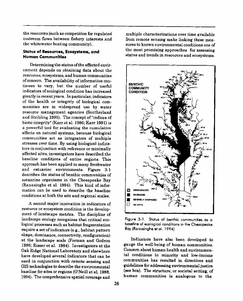
Determining the status of the affected envir-onment depends on obtaining data about theresources, ecosystems, and human communitiesof concern. The availability of information con-tinues to vary, but the number of usefulindicators of ecological condition has increasedgreatly in recent years. In particular, indicatorsof the health or integrity of biological com-munities are in widespread use by waterresource management agencies (Sutherlandand Stribling 1995). The concept of “indices ofbiotic integrity” (Karr et al. 1986; Karr 1991) isa powerful tool for evaluating the cumulativeeffects on natural systems, because biologicalcommunities act as integrators of multiplestresses over time. By using biological indica-tors in conjunction with reference or minimallyaffected sites, investigators have described thebaseline conditions of entire regions. Thisapproach has been applied to many freshwaterand estuarine environments. Figure 3-1describes the status of benthic communities ofestuarine organisms in the Chesapeake Bay(Ranasinghe et al. 1994). This kind of infor-mation can be used to describe the baselineconditions at both the site and regional scales.

A second major innovation in indicators ofresource or ecosystem condition is the develop-ment of landscape metrics. The discipline oflandscape ecology recognizes that critical eco-logical processes such as habitat fragmentationrequire a set of indicators (e.g., habitat patternshape, dominance, connectivity, configuration)at the landscape scale (Forman and Godron1986; Risser et al. 1984). Investigators at theOak Ridge National Laboratory and elsewherehave developed several indicators that can beused in conjunction with remote sensing andGIS technologies to describe the environmentalbaseline for sites or regions (0’Neill et al. 1988,1994). The comprehensive spatial coverage and

multiple characterizations over time availablehorn remote sensing make linking these mea-sures to known environmental conditions one ofthe most promising approaches for assessingstatus and trends in resources and ecosystems.

BENTHIC ~.a ‘QsCOMMUNITY

*CONDITION ~~>

-=$gMIT.2

a!-%?k

ET-9it!i 2T.1O

w

$fj UNDEGRADED

B DEGRADED““’::$$~n

~ SEVERELV DEQRADED

C22.2

I E.c&7

Figure 3-1. Status of benthic communities as abaseline of ecological conditions in the Chesapeake

Bay (Ranasinghe et al. 1994)

Indicators have also been developed togauge the well-being of human communities.Concern about human health and environmen-tal conditions in minori~ and low-incomecommunities has resulted in directives andguidelines for addressing environmental juetice(see box). The structure, or societal setting, ofhuman communities ie analogous to the

26

structure of a natural ecosystem. Human com-munities are integrated entities with character-istic compositions, structures, and functioning.The community profile draws upon indicators ofthese aspects to describe the integrity of thecommunity (FHWA 1996). Community indica-tors can range from general variables such as“social service provision” to specific indicatorssuch as “distance to nearest hospital.” Indica-tors can also be composites of different factors.For example, the familiar “quality of life” indi-cator is an attempt to merge key economic,

EnvironmentalJustice

In 1994, PresidentClinton issued Executive

Order 12398, “Federal Actions to AddweEmitmmmtcJ kstke in Minority Populotkwand Low-{ ncorne Populations,* requiring

federal agencies to udopt strategies to uddras

envirortmentaf @ice concerns within the

context of ogertq operations. 10 an accom-

panying memorandum, the President

emphasizes that existing faws, including NEPA

provide opportunities for federal o~encies to

address this issue. The U.S. EPA has stated

that addressing environmental justice concern,

is entirely consistent with NEPA and that dis-

proportionately high and adverse human

health or environmental effects cm minority or

low-income populations should be analyzedwith the same tools currently intrinsic to the

NEPA process, Specifically, the analysis

should focus on smaller areas or communities

within the affected area to identify significant

effects that may otherwise have been diluted

by an examination of a larger population or

area. Oemogrcaphic,geographic, economic,

cmd human health and risk factors all con-

tribute to whether the populations of concern

face di$pmportionately high and adverse

effects. Public involvement is particularly

important for idenfifyhg the aspects of minor-

ity and low-income communities thot need to

be addressed. Early and sustained cammuni~

cations with the aff&ted community through-

out the NEPA process is an essential aspect of

environmental iustice.

cultural, and environmental factors into anoverall characterization of community well-being.

Characterization of Stress Factors

Environmental impact assessment is anattempt to characterize the relationship be-tween human activities and the resultantenvironmental and social effects; therefore, thenext step in describing the affected environmentis to compile data on stress fkctors pertaining toeach resource, ecosystem, and human commun-ity. Table 3-1 lists 26 activities (both existingand proposed), in addition to the proposedaction, that may cumulatively affect resourcesof concern for the Castle Mountain MiningProject (U.S. BLM 1990). For each activity inthis example, anticipated cumulative effects areidentified for each of 12 resource issues. Theprimary locations of expected effects are alsolisted. The analyst should use this kind ofstress information to summarize the overalladverse effect on the environment. Analo-gously, other activities that benefit the environ-ment (e.g., restoration projects) should be in-cluded to determine the overall net (adverse orbeneficial) effect on the environment. Whereactivities contributing to cumulative effects areless well defined, a general stress level can bedescribed. For instance, the affected environ-ment discussion need not address every farm inthe watershed, but it should note the presenceof substantial agricultural activity.

Two types of information should be used todescribe stress factors contributing to cumu-lative effects. First, the analyst should identi~the types, distribution, and intensity of keysocial and economic activities within the region.Data on these socioeconomic “driving variables”can identify cumulative effects problems in theproject area (McCabe et al. 1991). For example,population growth is strongly associated withhabitat loss. A federal proposal that would con-tribute to substantial population growth in aspecific region (e.g., a highway project travers-ing a remote area) should be viewed as a likelydriving variable for environmental effects.

27

Table 3-1. Other activities (existing and proposed) that may cumulatively affect resources ofconcern for the Castle Mountain Mining Proiect (U.S. BLM 1990)

AnticipatedEnvironmental

Primary ImpactDescription/Responsible Agency Status Issues That Could

Be CumulativeLocation

lhiliti&s/Semites

1 AT&T Communication cable upgrading (BLMN) E,P 4,1 Iv

2 PocBellmicrowave sites (BIA4N) E,P 4,1 Iv

3 Bio Gen power plant (SBC) E 2 Iv

4 Additional utility lines (1 -15 corridor) (BLMN) P 4,4 Iv

5 Whiskey Pete’s airslrip/waterline (BLMN) P 4 Iv

6 Salid woste landfill (UP Tracks near state line) (BLMN) P- 4,12 Iv

7—.-

Waste water ponds (Ivanpoh Lake) (BLMN)-– t— .–~––~ --— -

4,9 IV

i Nipton woste site (BIA4N) P 4,9 Iv

? IA-Los Vegas bullet train (BLMN) P – 4,9,10 &

Commercial and Residenficsl——

10 Nipton land exchonge (BLMN) P 4,6,12~~v—–—

11 Sccs~eredresidential units (BLMN) E,P - . . LV

?ecreaticm

12 Ivanpah Lake landsailing (BLMN) E 4,5,10 Iv

13 Borstow to Vegas ORV race (BLMN) E 4,5,10 Iv

14 East Molave Heritage Trail use (BLMN) E 4,5,10 I~L~ W

15 Molave Road use (BLMN) E 4,5,10 l~L~W –~ Clark Country Rood A6BP use (BLMS,CC) E 4,5,10 w

A4ining

17 Proposed Action/Alternative - precious metals (BLMN) I P 3,4,5,8,9 LV

~8 Calasseum Mine - preciaus metals (BIJAN) E 3,4,5,8,9 Iv

19 Caltrans borrow pits - aggregates (BLMN) E 4,5 Iv

20 Morning Star Mtne - preciaus metals (BLMN) E 3,4,5,8,9 Iv

21 Vanderbilt - precious metals mill site (BIMN) E 3,4,5,8,9 Iv

22 Golden Quail Mine - preciaus metals (BLMN) E 34589,,, , LV

23 Hart District Clay Pits (BLMN) E 4,9 LV

24 Mountain pass Mine - rare earth materials (BLMN) E 3,4,5,8,9 Iv.—25 Explorato~ activities (BLMN, BLMS) E,P 1, 4,5,9 L~W

&azing

?6 Grazing leases (BLMN, BLMS) E 4,5 Iyv, w

kurce of Inhrmatian Status IssuesN-MN: BLM Needles E: Existing

Location1 Earth

NA4S: BLM StatelinefW Piute Valley

P Propased 2 Air IV Ivan ah Valley;BC: San Bernardino County. Planning Department 3 Water FSC: Clark County, Planning Department

LW Lan air Valley4 Wildlife5 Vegetation6 Transportation7 Public Sewice/Utilities ,8 Health/Safety9 Visual Resaurces10 Recreation11 Cultural Resources12 Land Use

Second, the analyst should look for indi-vidual indicators of stress on specific resources,ecosystems, and human communities. Like thefamiliar “canary in the coal mine,” changes incertain resources can serve as an early warningof impending environmental or social degrada-tion (Reid et al. 1991). Indicators of environ-mental stress can be either exposure-oriented(e.g., contamination levels) or effects-oriented(e.g., loss or degradation of a fishery). High sed-iment loads and the loss of stable stream banksare both common indicators of cumulativeeffects from urbanization.

The goal of characterizing stresses is todetermine whether the resources, ecosystems,and human communities of concern are ap-proaching conditions where additional stresseswill have an important cumulative effect.Simple maps (Figure 3-2) of existing andplanned activities can indicate likely cumu-lative effects, as in the example of Seattle’sSouthwest Harbor (USACE et al. 1994).Regulatory, administrative, and planning inform-ation can also help define the condition of theregion and the development pressures occurringwithin it. Lastly, trends analysis of change inthe extent and magnitude of stresses is criticalfor projecting the future cumulative effect.

Regulations, Administrative Standards,and Regionai Plans

Government regulations and administrativestandards (e.g., air and water quality criteria)can play an important role in characterizing theregional landscape. They often influence devel-opmental activity and the resultant cumulativestress on resources, ecosystems, and humancommunities. They also shape the manner inwhich a project maybe operated, the amount ofair or water emissions that can be released, andthe limits on resource harvesting or extraction.For example, designation of a “Class I“ airquality area can restrict some types of devel-opment in a region because the Prevention ofSignificant Deterioration (PSD) requirementestablishes a threshold of cumulative air qual-ity degradation,

29

In the United States, agencies at manydifferent levels of government share respon-sibilities for resource use and environmentalprotection. In general, the federal governmentis charged with functions such as nationalstandard-setting, whereas state governmentsmanage implementation by issuing permits andmonitoring compliance with regulatory stan-

dards. Each of the states handles environ-mental regulation and resource management inits own way. Most states have chartered spe -cific agencies for environmental protection, re -source management, or both. This information,along with contact names, can be obtained fromthe Council of State Governments (Brown andMarshall 1993). States usually have discretionunder federal law to set standards more strin-gent than national ones. Land-use decisions areusually made by local governments. Local con-trol may take the form of authority to adoptcomprehensive land use plans; to enact zoningordinances and subdivision regulations; or torestrict shoreline, floodplain, and wetlanddevelopment. Data on local government issuesand programs can be obtained through relevantlocal government agencies.

The affected environment section of a NEPAanalysis should include as many regulations,criteria, and plans as are relevant to the cumu-lative effects problems at hand. Federal, state,and local resource and comprehensive plansguiding development activities should be re-viewed and, where relevant, used to completecharacterization of the affected environment.Agencies’ future actions and plans pertaining tothe identified resources of concern should be in-cluded if they are based on authorized plans orpermits issued by a federal, state, or other gov-ernmental agency; highly speculative actionsshould not be included. Agency or regionalplanning documents can provide the analystwith a reasonable projection of future activitiesand their modes of operation. How projecteffects fit within the goals of governmental reg-ulations and planning is an important measureof cumulative effects on the resources, ecosys-tems, and human communities of the region.

- Im+==f

M l?-]t —mm

u.

L– I I I

.-Ih

9NoTTascm

Figure 3-2. Regional map of proiects and activities contributing to cumulative effects in Seaitle’s Southwest Harbor

(USACE et al. 1994)

30

Trends

Cumulative effects occur through the ac-cumulation of effects over varying periods oftime. For this reason, an understanding of thehistorical context of effects is critical toassessing the direct, indirect, and cumulativeeffects of proposed actions. Trends data can beused in three ways: (1) to establish the baselinefor the affected environment more accurately(i.e., by incorporating variation overtime), (2) toevaluate the significance of effects relative tohistorical degradation (i.e., by helping to esti-mate how close the resource is to a threshold ofdegradation), and (3) to predict the effects of theaction (i.e., by using the model of cause andeffects established by past actions).

The ability to identify trends in conditionsof resources or in human activities depends onavailable data. Although data on existing con-ditions can sometimes be obtained for cumu-lative effects analysis, analysts can rarely goback in time to collect data (in some cases, lakesediment cores or archaeological excavationscan reconstruct relevant historical conditions).Improved technologies for cost-effectivelyaccessing and analyzing data that have beencollected in the recent past, however, have beendeveloped. Historical photographs and re-motely sensed satellite information can beefficiently analyzed on geographic informationsystems to reveal trends. The analyst may usethese tools to characterize the condition of aresource before contemporary human influ-ences, or the condition at the period whenresource degradation was first identified. Asshown in Figure 3-3, remote sensing imagerywas used to record the change in the conditionof the Jemez Mountains, New Mexico (Allen1994). The 1935 map (left) shows the location ofrailroads, dirt roads, and primitive roads in thelandscape surrounding the Bandelier NationalMonument. By 1981 (right) the increase inroads and the appearance of several townsitesis striking.

This 12-fold increase in total road length isan effective measure of cumulative environmen-tal degradation resulting from the accompany-ing fire suppression, motorized disturbance ofwildlife, creation of habitat edge in forestinteriors, and introduction of weedy speciesalong road corridors. The U.S. Forest Servicehas been using this landscape-scale GIS andremotely sensed information in planning effortsfor the Bandelier’s headwaters area to ensurethat desired forest conditions are maintained(e.g., area and distribution of old growth anddensities of snags).

OBTAINING DATA FOR CUMULATIVEEFFECTSANALYSIS

Obtaining information on cumulative effectsissues is often the biggest challenge for the ana-lyst. Gathering data can be expensive and timeconsuming. Analysts should identifj whichdata are needed for their specific purpose andwhich are readily available. In some cases,federal agencies or the project proponent willhave adequate data; in other cases, local orregional planning agencies may be the bestsource of information. Public involvement canoften direct the analyst to useful information or,itself, serve as an invaluable source of informa-tion, especially about the societal setting, whichis critical for evaluating effects on human com-munities. In any case, when information is notavailable from traditional sources, analystsmust be resourceful in seeking alternativesources. Table 3-2 lists some of the possibletypes and sources of information that maybe ofuse for cumulative effects analysis.

Although most information needed todescribe the affected environment must beobtained from regional and local sources, sev-eral national data centers are important.Census Bureau publications and statisticalabstracts are commonly used for addressingdemographic, housing, and general socioeco-nomic issues, as are several commercialbusiness databases. Currently, an extensiveinventory of environmental data coordinated by

31

The Nature Conservancy through state NaturalHeritage Programs (NHPs) and ConservationData Centers (CDCS) provides the mostcomprehensive information available about theabundance and distribution of rare species andcommunities (Jenkins 1988). NHPs and CDCSare continually updated, computer-assistedinventories of the biological and ecologicalfeatures (i.e., biodiversity elements) of theregion in which they are located. These datacenters are designed to assist in conservationplanning, natural resource management, andenvironmental impact assessment. Anotherpromising source of data is the U.S. Geological

by the consolidation of biological research,inventory and monitoring, and informationtransfer programs of seven Department ofInterior bureaus. The mission of the Division isto gather, analyze, and disseminate the biolog-ical information necessary to support soundmanagement of the nation’s resources. The U.S.Geological Survey itself was originally createdin response to the demands of industry andconservationists for accurate baseline data.Although substantial information can alreadybe obtained horn USGS, the implementation ofthe National Biodiversity Information Infra-structure (NAS 1993) may provide even greater

Survey’s Biological Resources Division, created access to comprehensive biological data,

“$.... ...”..... ............;

,..,’[ w.............. N

.,$. . . . f’::. ‘--......

o s 10

kilometers

1981

Figure 3-3. Remote sensing imagery illustrating the cumulative increase in roads between 1935 and 1981 across

the same 187,858 ha of the Jemez Mountains, New Mexico. The crosshatched line is a railroad; the solid lines

are dirt roads; the thin dashed lines are primitive roads’ and dotted lines show the current boundary of Bandelier

National Monument (Allen 1994),

32

Table 3-2. Possible sources of existing data for cumulative effects analysis

Individuals ■ former and present landholders● Iong-t[me residents■ Iong-t!me resource users● long-time resource managers

Historical societies Local, state, and regional societies provide:● personal Iournals■ photos■ newspapers■ indiwdual contacts

Schools and universities ■ central libraries■ natural history or cultural resources collections ar museums■ field stations■ faculty in hwtory and natural and social sciences

Other collections Private, city, state, or federal collections in :● archaeology■ botany~ zaolag

{“● natura history

Natural history suweys ■ private■ state■ national

Private organizations ■ land preservation■ habitat preservation■ conservation■ cultural resources history■ religious institutions■ chambers of cammerce■ volunta~ neighborhood organizations

Government agencies ■ local park districts .. local plannm~ag~cles■ local records- ee mg agencies■ state and federal and management agencies■ state and federal fish, wildlife, and conservation agencies■ state and federal regulatory agencies I■ state planmng a encles

Y■ state and federa records-keeping agencies■ state and federal suryeys■ state and federal agricultural. and forestry agencies■ state hlstorlc preservation offtces■ Indian tribal government planning, notural resource, and cultural resource affices

Proiect proponent ■ proiect dam and supporting environmental documentation

Although federal data sources are critical integration of data (Irwin and Rades 1992). Thefor compiling baseline data, they have sub- only comprehensive effort to develop estimatesstantial-limitations. For the most part, federalenvironmental data programs have evolved tosuppart a specific agency’s missions. They arenot designed to capture the interconnectionsamong environmental variables or generateinformation needed for analyses that cut across

sectorial and disciplinary lines. The fact thatfederal databases are often generated by moni-toring programs designed to track progress inmeeting regulatory goals further inhibits

of baseline ecological conditions across theUnited States has been the EnvironmentalMonitoring and Assessment Program (lMI.AP).EMAP has successfully developed indicators formany resources and has applied them inregional demonstration programs to providestatistically rigorous estimates of the conditionof ecosystems. Fully implemented, this pro-gram would be invaluable for analyzing cumu-lative effects (see box).

33

13diaillgmi$ii1ihi9 w&#ji@iliCmdithm mrcwgh WAP

Over fhe M decade, EPA has ied a rr@i@en~ effm-t to assess the Gonditkm of the rmfian’s

IWYA&Ul rewtirces {MWW et cd, 1991), Yh~:Envitonm@c+l A4tmitoringj tmd Asswsment Progmrn

(EJA@]’s goal is “to identify the extent.pn~ ~agriii~e of ~nvircmmemt~l prablaw cm re$icmal andnational scchs and fu pt’uvide infsrm&o that Wliimakem, @mtkts, and’fhepublicntiedfOtiluafethewccws of environmental policim and praqrams fl%ornfcm et cd<19%4], WAP hcwdevkkped Qscientifically rigorous monitoring deisiqn. @mrton et al. 195@) witldn which upproprikde Irtdicofms

(Burbw 19?4) canbe:scm#A trwovIds X* typtqof informotkmr+uirtid to oddress thesa questions.EMAP MM WMXISSMly~ld tastdmpny of the’hxlkatcws, samplin~protocols,and assessment methods

required to evaluate the ccqdtion of indh+idued tscek-agiccd msmJr@ ffmtien and Chrisfie 1993;

$ummem et al, 1993; V&dsb~ @ cd. 1993; “lmwis and Conklim 1994], Although intimates of the

ccmdition of certain resouwes have Wn **I+ for w%dn mgiom, EW “hasnot yet beenimpienmntd on a IQrge scale,

EMAP difbrs from ofher mafiitmin~ pro~roms in tlm following ways:

B WAP focuses on assessing. ecok@cxd condition by measuring biological indicators,8i010$ical indic@W’s

fRrmiichs irt~tatii rniwasure~ of respome to natural and

human-induced stress at cannq be obtained f~m frcdificmal chemical and physical.indicatum of, environmental strews W& w pcdfutanfs und Iw@iiat modification. Thepro ram maIntolM a core set of indhhr$ that arb in@6ir@ed natianaliy with uniform

Jm : cdolo~ and quality control,.

K IWAP wos q @@i@6fly ri~wws .som”li~ desiiqn, ~By measwinq indicators within u$network of prababMy scm@Qs rather m Jrom shs deck. using subjective criteria,

EAW produ- ~bid astimates of the status of utid chtm~es in indicators of ecologicalctmditicm wi~: known ew$idwws.

■ ~P takes an qcosystem+wianfed approach to,monitwitigby~ctmpli~ sewral ecologicalresources< EMAP meintai.ns.moti~ng db-ls .itt C@dtw’til kmd$, rungelands{ %rwsts,estuaries, and surface waf*rS, $.*.,. H@ss and sfreams], * alsa maintajns cross-cuttingocfivifies in ksndscape daracteiizatien, iridhtor d@opm@n$ cd atmospheric depodticm.

Them attributes m~ke EW wdquely sdtisd to uddnsssing cumukttlve effects. Where regional

estirnafes of ecol~iccd cotwlitian h~vet beitt de@aped, thqy tin be used os “baselirw condtiions forevaluating the effects of new p@scts. Afthbugh ~P moniforin~is ~uw9nt@limitedto a few regions

of#MJCQUntW4 the W cqqmach is MHQ a@id ta stafe monitoring “k+fkxtsthatw“IIestablish baseline

condfikm(m &wPwrlundandWei$be~ 1MM for opplicoticm to Marykmdstrenms),

AFFECTED ENVIRONMENT SUMMARY

The description of the affected environmenthelps the decisionmaker understand the cur-rent conditions and the historical context of theimportant resources, ecosystems, and humancommunities. The analyst uses this phase ofthe NEPA process to characterize the regionand determine the methodological complexityrequired to adequately address cumulative

effects. In describing the affected environment,the cumulative effects analyst should

identify common cumulative effectsissues within the region;

characterize the current status of theresources, ecosystems, and human com-munities identified during scoping;

identi& socioeconomic driving variablesand indicators of stress on these re-sources;

34

■ characterize the regional landscape in The affected environment section shouldterms of historical and planned devel- include data on resources, ecosystems, andopment and the constraints of govern- human communities; environmental and socio-mental regulations and standards; and economic stress factors; governmental regula-

■ define a baseline condition for the re- tions, standards, and plans; and environmental

sources using historical trends. and social trends. This information will providethe analyst with the baseline and historicalcontext needed to evaluate the environmentalconsequences of cumulative effects (Chapter 4).

35

4DETERMINING THE ENVIRONMENTALCONSEQUENCES OF CUMULATIVE EFFECTS

PRINCIPLES

D Addr= c@ditlve, countetvaMingi and

synergkfic effects.

m Lti @y~d ~ Ii@ d the CICflQ~.

u Mt= ths sustdndMIWOfwweescecosystems, and human cornmunltles.

The diversity of proposed federal actionsand the environments in which they occur makeit difficult to develop or recommend a singlemethod or approach to cumulative effects anal-ysis. In this chapter, we attempt to provideinsight into and general guidelines for per-forming analyses needed to determine theenvironmental consequences of cumulativeeffects. We assume the analysis has alreadybeen scoped, including stipulating geographicand time boundaries (see Chapter 2), and thatappropriate data have been gathered for theresources, ecosystems, and human communitiesof concern (see Chapter 3). Reference is made,when appropriate, to specfic cumulative effectsanalysis methods described in Chapter 5 andAppendix A.

The analyst must ensure that the resourcesidentified during scoping encompass all thoseneeded for an analysis of cumulative effects.The analyst must also ensure that the relevantpast, present, and reasonably foreseeable future

37

actions have been identified. As an iterativeprocess, cumulative effects analysis often iden-tifies additional resources or actions involved incumulative effects during the analysis phase.In addition to confirming the resources andactions to be considered, the analyst shouldcomplete the following specific steps to deter-mine the environmental consequences of thecumulative effects:

m

mIEiiElEiiizl

Identify the important cause-and-effect relationships betweenhuman activities and resources,ecosystems, and human com-munities.

Determine the magnitude andsignificance of cumulative effects.

Modify or add alternatives toavoid, minimize, or mitigate sig-nificant cumulative effects.

Monitor the cumulative effects ofthe selected alternative and adaptmanagement.

CONFIRMING THE RESOURCES ANDACTIONS TO BE INCLUDED IN THE CUMU-LATIVE EFFECTS ANALYSIS

Even though scoping has identified likelyimportant cumulative effects, the analystshould include other important cumulativeeffects that arise from more detailed consider-

ation of environmental consequences. Inaddition, as the proposed action is modified orother alternatives are developed (usually toavoid or minimize adverse effects), additional ordifferent cumulative effects issues may arise.Specifically, the proposed action and reasonablealternatives (including the no-action alterna-tive) could affect different resources and couldaffect them in different ways. For instance,hydroelectric facilities primarily affect aquaticresources by blocking fish migration routes,altering thermal regimes, and eroding streamchannels as releases fluctuate. Reasonablealternatives for proposed hydroelectric facilitiesoften include various types of power generatingfacilities that affect the environment in dif-ferent ways. For example, the effects of coal-fired electric plants are most often related tocoal-mining activities, the release of heatedwater to nearby water bodies in the coolingprocess, and the release of a variety of pol-lutants (including greenhouse gases) to the airduring combustion. Nuclear plants also releaseheated water but they release radioactivematerials to the air instead of greenhousegases. Other past, present, or future actionsalso should be included in the analysis ifevaluation of the cause-and-effect relationshipsidentifies additional stresses affecting re-sources, ecosystems, and human communitiesof concern.

IDENTIFYING AND DESCRIBING CAUSE-AND-EFFECT RELATIONSHIPS FORRESOURCES, ECOSYSTEMS, AND HUMANCOMMUNITIES

In preparing any assessment, the analystshould gather information about the cause-and-effect relationships between stresses and re-sources. The relationship between the percentof fine sediment in a stream bed and the emer-gence of salmon fly (Figure 4- 1) is an example ofa model of cause and effect that can be usefulfor identi&ing the cumulative effects on aselected resource. Such a model describes theresponse of the resource to a change in itsenvironment. To determine the consequences of

the proposed action on the resource, the analystmust determine which cumulative environmen-tal changes (e.g., higher sediment load) willresult from the proposed action and otheractions.

la) I (

o 20 40 60 00 160

Percent Fine Sediment

Figure 4-1. Empirical cause and effect relationship

between emergence of salmon fry and percent of

fine sediment in the stream bottom (Stowell et al.

1983)

Determining the Environmental Changesthat Affect Resources

Using information gathered to describe theaffected environment, the factors that affectresources (i.e., the causes in the cause-and-effect relationships) can be identified and aconceptual model of cause and effect developed.Networks and system diagrams are the pre-ferred methods of conceptualizing cause-and-effect relationships (see Appendix A). The ana-lyst can develop this model without knowingprecisely how the resource responds to environ-mental change (i.e., the mechanism of thecause-and-effect relationship). If all pathwaysare identified, the model will be quite complex(Figure 4-2). Such a complex model can seldombe fully analyzed because sufficient data usu-ally are not available to quanti& each pathway.Because of this, the model should be simplifiedto include only important relationships that canbe supported by information (Figure 4-3).

38

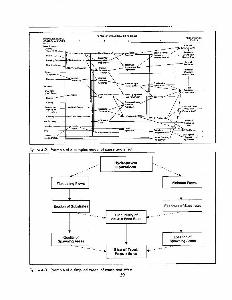
RESPONSEVARIABLESANDPROCESSESMANAGECVEXTERNAL RESOURCWSECONTROLVARIABLES ,. ~ ~. ~. STATUS

Figure 4-2. Example of a complex model of cause and effect

PFluctuating Flows

HydropowerOperations

I I

aErosion of Substrates

--”1 Productivity ofAquatic Food Base

k

+

Quality ofSpawning Areas

1

Size of TroutPopulations

?

Exposure of Substrates

t IwFigure 4-3. Example of a simplied model of cause and effect

39

The cause-and-effect model can aid in theidentification of past, present, and futureactions that should be considered in the analy-sis. In the example shown in Figure 4-3, theanalyst should determine if there are otherprojects in the area that would affect any of thecause-and-effect pathways. The cause-and-effect model for the cumulative effects analysiswill often include pathways that would not beneeded for a project-specific analysis. Thus, asin defining boundaries, analyzing the conse-quences of cumulative effects requires broaderthinking about the interactions among theactivities and resources that affect environ-mental change.

Determining the Response of the Resourceto Environmental Change

Once all of the important cause-and-effectpathways are identified, the analyst shoulddetermine how the resource responds to envir-onmental change (i.e., what the effect is). Thecause-and-effect relationships for each resourceare used to determine the magnitude of thecumulative effect resulting from all actionsincluded in the analysis.

Cause-and-effect relationships can be sim-ple or complex. The magnitude of an effect on aspecies may depend simply on the amount ofhabitat that is disturbed. Similarly, effects onarchaeological sites may be quantified by enum-erating the sites that are disturbed. Otherresponses may be more complex. The exampleshown in Figure 4-1 demonstrated that the suc-cessful hatching of salmon eggs depends on thepercentage of fine particles in the stream bot-tom in a complex but predictable fashion. Socio-economic models can be applied in a similarway to determine the effects of changes inimmigration and emigration rates on the finan-cial condition of a human community.

A wide variety of cause-and-effect evalua-tion techniques have been described in theliterature (see Chapter 5). Techniques for eval-uating ecological resources include the set ofHabitat Suitability Index Models (HSI;

Schamberger et al. 1982; Hayes 1989) developedby the U.S. Fish and Wildlife Service for itsHabitat Evaluation Procedures (HEP; U.S. Fishand Wildlife Service 1980). These models usecause-and-effect relationships for several keyenvironmental variables to determine the suit-ability of different habitats for a variety ofspecies. The change in number of habitat units(i.e., the ability of an area to support a species)as a result of multiple actions is a usefulmeasure of cumulative effects. Species habitatmodels also drive the Habitat EvaluationSystem of the U.S. Army Corps of Engineers(1980). For wetland habitat designations, theWetland Evaluation Technique is often used(Adamus et al. 1987). Other methods for link-ing measures of environmental change to effectson resources include developing relationshipsbetween loss in wetland area and functionssuch as flood storage, water quality, and lifesupport (Preston and Bedford 1988; Leibowitzet al. 1992) and linking hydrology first tovegetation and then to wildlife habitat (Nestler1992).

Nonlinear cause-and-effect relationshipsamong several environmental changes pose anadditional challenge for the analyst. A commonexample is the synergistic effect on fish popula-tions that results from the combination of directmortality losses to hydropower turbines andincreased predation losses that occur as preda-tors are attracted to dead and stunned fish. Theanalyst may also have to predict additional fishmortality horn disease as a result of reductionsin immune responses caused by toxic contami-nation. A third example of a common cumula-tive cause-and-effect problem is the combinedeffect on dissolved oxygen levels of excessivealgal growth resulting from both increasednutrient loading and higher temperatures.

One of the most useful approaches for deter-mining the likely response of the resource, eco-system, and human community to environmen-tal change is to evaluate the historical effects ofactivities similar to those under consideration.In the case of road construction through a

40

forest, the effects of similar past actions such asthe construction of pipelines and power linesmay provide a basis for predicting the likelyeffects of the proposed road construction. Theresidual effects of constructing and operatingthese linear facilities include fragmentation offorest tracts and the creation of homogeneousvegetation in the rights-of-way. Trends analy-sis (see Appendix A) can be used to model theeffects of linear facilities over time andextrapolate the effects of a road constructionproject into the future.

If cause-and-effect relationships cannot bequantified, or if quantification is not needed toadequately characterize the consequences ofeach alternative, qualitative evaluation proce-dures can be used. The analyst may categorizethe magnitude of effects into a set number ofclasses (e.g., high, medium, or low) or provide adescriptive narrative of the types of effects thatmay occur. Often, the analyst will be limited toqualitative evaluations of effects because cause-and-effect relationships are poorly understoodor because few site-specific data are available.Even when the analyst cannot quanti~ cumu.lative effects, a useful comparison of relativeeffects can enable a decisionmaker to chooseamong alternatives.

DETERMINING THE MAGNITUDE ANDSIGNIFICANCE OF CUMULATIVE EFFECTS

The analyst’s primary goal is to determinethe magnitude and significance of the environ-mental consequences of the proposed action inthe context of the cumulative effects of otherpast, present, and fiture actions. To accom-plish this, the analyst must use a conceptualmodel of the important resources, actions, andtheir cause-and-effect relationships. The crit-ical element in this conceptual model is definingan appropriate baseline or threshold conditionof the resource, ecosystem, and human com-munity beyond which adverse or beneficialchange would cause significant degradation orenhancement of the resource, respectively.

The concept of a baseline against which tocompare predictions of the effects of the pro-posed action and reasonable alternatives is crit-ical to the NEPA process. The no-actionalternative is an effective construct for this pur-pose, but its characterization is often inade-quate for analyzing cumulative effects. Much ofthe environment has been greatly modified byhuman activities, and most resources, ecosys-tems, and human communities are in the pro-cess of change as a result of cumulative effects.The analyst must determine the realistic poten-tial for the resource to sustain itself in thefuture and whether the proposed action willaffect this potential; therefore, the baselinecondition of the resource of concern shouldinclude a description of how conditions havechanged over time and how they are likely tochange in the future without the proposedaction.

The potential for a resource, ecosystem, andhuman community to sustain its structure andfunction depends on its resistance to stress andits ability to recover (i.e., its resilience). Deter-mining whether the condition of the resource iswithin the range of natural variability or isvulnerable to rapid degradation is frequentlyproblematic. Ideally, the analyst can identifi athreshold beyond which change in the resourcecondition is detrimental. More often, theanalyst must review the history of that resourceand evaluate whether past degradation mayplace it near such a threshold. For example, theloss of 50% of historical wetlands within awatershed may indicate that further losseswould significantly affect the capacity of thewatershed to withstand floods. It is often thecase that when a large proportion of a resourceis lost, the system nears collapse as the surviv-ing portion is pressed into service to performmore functions.

The baseline condition should also includeother present (ongoing) actions. For example,the National Ambient Air Quality Standards(NAAQS) inventory represents the universe of

41

present actions used in air quality analyses todetermine whether new emission sources willexceed air quality standards. The NAAQSinventory includes all existing emission sources,sources with Prevention of SignificantDeterioration (PSD) permits that have not yetbegun to operate, and applicants for whom aPSD permit has not yet been issued. TheNAAQS analysis requires explicitly modelingall existing nearby sources (as far away as 50kilometers) be for air quality effects. In theanalysis of the cause-and-effect relationshipsrelated to the anticipated impacts, each sourcerepresents a cause, and their combined emis-sions create an effect on air quality, the signif-icance of which can be determined by comparingthe concentration of pollutants emitted to thres-hold concentrations specified in the NAAQS.The NAAQS thresholds are concentrationsknown to cause significant human health orother environmental effects.

The historical context and full suite of on-going actions are not only critical for evaluatingcumulative effects, but also for developing po-tential restoration as well. The first step indeveloping a river restoration plan is to under-stand how past actions (e.g., contributions ofcontaminants to the watershed) have contrib-uted to the current condition of the water body.The historical trends in resource condition andits current potential for sustained structure andfunction are an essential frame of reference fordeveloping mitigation and enhancement mea-sures.

Determining Magnitude

Initially, the analyst will usually determinethe separate effects of past actions, presentactions, the proposed action (and reasonablealternatives), and other future actions. Onceeach group of effects is determined, cumulativeeffects can be calculated. The cumulativeeffects on a specific resource, however, will notnecessarily be the sum of the effects of all

actions. Knowing how a particular resourceresponds to environmental change (i.e., thecause-and-effect relationship) is essential fordetermining the cumulative effect of multipleactions. Will the effects of two or more actionsbe additive, i.e., if one project would result inthe death of 25’%0of a trout population (within agiven level of uncertainty) and another thedeath of 10% of the trout, would the two projectstogether result in the loss of 35V0of the trout?Although this is sometimes the case, there areoften instances where the cause-and-effect rela-tionship is more complex, i.e., the cumulativeeffect of two projects may be greater than thesum of the effects of each (in the trout example,more than 35% of the trout would die) or lessthan their sum (less than 35% of the troutwould die). In some cases, the resource maybetter withstand additional adverse effects asstress increases, while in others, the resourcemay crash once a threshold is reached.

Once effects are identified using one of themethodologies described in Chapter 5, a tablecan be used to itemize effects into categories ofpast, present, proposed, and future actions.Tables 4-1, 4-2, and 4-3 show how these tablescan be constructed using the results horn differ-ent types of analyses. Regardless of the degreeof quantification used, such tables are usefultools for putting the effects of the proposedaction and alternatives into proper context.Table 4-1 illustrates the net cumulative effectsof combining fish population increases from theproposed action with population losses frompast and future actions. The table could be ex-panded to include the countervailing effect ofsulfate aerosols on global warming (becausethey compensate for greenhouse gases) at thesame time they are degrading ambient air qual-ity. A series of such tables (one for each altern-ative) enables the analyst to compare alterna-tives meaningfully.

42

Table 4-1. Example table using quantltatke description of effects (within a given level ofuncertainty) on various resources

ResourceCumulative

Past Actions Present Actions Proposed Action Future ActionsEffect

Air Quality No effect on S02 20% increase in S02 1O% increase in S02 5% increase in S02 35% increase in

so,

Fish 50% of 1950 2% of fish 5% increase in fish 1% of fish 48% af 1950 fish

population lost population lost population population lost population lost

Wetlands 78% af presettlement 1% of existing 0.5% of existing 1 .5% of existing 95% of preset-

wetlands lost wetlands lost wetlonds lost wetlands lost annu- tlement wetlands

annually far 5 years ally for 10 years lost inl O years

The separation of effects into those attribu-table to the proposed action or a reasonablealternative versus those attributable to pastand future actions also allows the analyst todetermine the incremental contribution of eachalternative. Situations can arise where anincremental effect that exceeds the threshold ofconcern for cumulative effects results, not hornthe proposed action, but from reasonably fore-seeable but still uncertain future actions.Although this situation is generally unexplored,the decisionmaker is faced with determiningwhether to forgo or modi& the proposed actionto permit other future actions. Identifying in-cremental effects, therefore, is an importantpart of informing the decisionmaker.

Most cumulative effects analyses will iden-tifi varying levels of beneficial and adverseeffects depending on the resource and the indi-vidual action. Aquatic species will experienceentirely different effects from terrestrial ones.A warm water fishery (e.g., Iargemouth bass)may benefit from a change that is detrimentalto a cold water fishery (e.g., trout), and effectsthat are beneficial to the well being of a humancommunity (e.g., provision of social services)may be detrimental to natural systems (e.g.,wetlands lost during construction of a hospital).

Because of this mixture of beneficial andadverse effects, the decisionmaker is often hardpressed to determine which alternative is envir-onmentally preferred. To overcome this prob-lem, indices of overall cumulative effect can bedeveloped. Some of the matrix methods used incumulative effects analysis were developedspecifically to address this need. These methodsuse unitless measures of effect (e.g., scales orranks) to get around the problem of combiningresults from a variety of resources.

Presentation of overall cumulative effectscan be controversial. Intentional or uninten-tional manipulation of assumptions can dra-matically alter the results of aggregated indices(Bisset 1983), and experience indicates thatcomplex quantitative methods for evaluatingcumulative effects make it more diflicult for thepublic to understand and accept the results.Effects on resources are usually presentedseparately, and professional judgment is usedin determining the reasonable alternative withthe greatest net positive cumulative effect. TheU.S. EPA has developed guidelines for address-ing specific kinds of risks (including cancerrisks and the risks posed by chemical mixtures)and for comparing disparate kinds of risks (U.S.EPA 1993).

43

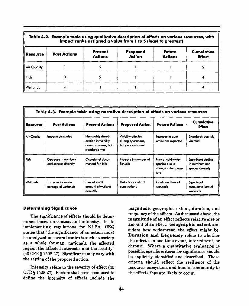
Table 4-2. Example table using qualitative description of effects on various resources, withimpact ranks assigned a vaiue from 1 to 5 (ieast to greatest)

i I I I I

Resource Past ActionsPresent Proposed Future CumulativeActions Adion Actions Effect

Air Quality 1 2 1 1 2

Fish 3 2 1 1 4

Wetlands 4 1 1 1 4I , 1 1 1

Tabie 4-3. Exampie tabie using narrative description of effects on various resources IResource

Air Qualify

Fish

Wetlands

Past Actiosss I Present Actions

Impacts dissipated

D-ease in numbers

and species diversity

Noticeable deteri-

oration in visibility

during summer, but

standards met

Occasional docu-

mented fish kills

Large reduction in I Lassof small

acreage of wetlands amount of wetland

annually

Determining Significance

The significance of effects should be deter-mined based on context and intensity. In itsimplementing regulations for NEPA, CEQstates that “the significance of an action mustbe analyzed in several contexts such as societyas a whole (human, national), the affectedregion, the affected interests, and the locality”(40 CFR $ 1508.27). Significance may vary withthe setting of the proposed action.

Intensity refers to the severity of effect (40CFR $ 1508.27). Factors that have been used todefine the intensity of effects include the

Proposed Action

Visibility affeded

during operations,

but standards met

Increme in number of

fish kih

Disturbance of a 5

acre wetland

Future ActionsCumulative

Effect

Increase in auto Standards possibly

emissions expectd violated

ILoss of cold-water Significant de&e

species due to in numbers and

change in tempera- Speciesdwersity

ture

Continued loss af i significant

wwtlands cumulative lass af

wetlands

magnitude, geographic extent, duration, andkquency of the effects, As discussed above, themagnitude of an effect reflects relative size oramount of an effect. Geographic extent con-siders how widespread the effect might be.Duration and frequency refers to whetherthe effect is a one-time event, intermittent, orchronic. Where a quantitative evaluation ispossible, specfic criteria for significance shouldbe explicitly identified and described. Thesecriteria should reflect the resilience of theresource, ecosystem, and human community tothe effects that are likely to occur.

Thresholds and criteria (i.e., levels of accept-able change) used to determine the significanceof effects will vary depending on the type ofresource being analyzed, the condition of theresource, and the importance of the resource asan issue (as identified through scoping). Cri-teria can be quantitative units of measure suchas those used to determine threshold values ineconomic impact modeling, or qualitative unitsof measure such as the perceptions of visitors toa recreational area. No matter how the criteriaare derived, they should be directly related tothe relevant cause-and-effect relationships.The criteria used, including quantitative thres-holds if appropriate, should be clearly stated inthe assessment document.

Determinations of significance in an EA oran EIS are the focus of analysis because theylead to additional (more costly) analysis or toinclusion of additional mitigation (or a detailedjustification for not implementing mitigation).The significance of adverse cumulative effects isa sensitive issue because the means to modificontributing actions are often outside the pur-view of the proponent agency. Currently,agencies are attempting to deal with this diffi-cult issue by improving their analysis of his-torical trends in resource and ecosystemcondition. Even where cumulative effects arenot deemed to be significant, better characteri-zation of historical changes in the resource canlead to improved designs for resource enhance-ment, Where projected adverse effects remainhighly uncertain, agencies can implement adap-tive management—flexible project implemen-tation that increases or decreases mitigationbased on monitoring results.

AVOIDING, MINIMIZING, ANDMITIGATING SIGNIFICANT CUMULATIVEEFFECTS

If it is determined that significant cumula-tive effects would occur as a result of a proposedaction, the project proponent should avoid,

minimize, or mitigate adverse effects bymodifiing or adding alternatives. The pro-ponent should not overlook opportunities toenhance resources when adverse cumulativeeffects are not significant. The separation ofresponsibilities for actions contributing tocumulative effects makes designing appropriatemitigation especially diflicult. In the case of theLackawanna Industrial Highway, the FederalHighway Administration and PennsylvaniaDepartment of Transportation sponsored devel-opment of a comprehensive plan for the valleythat provides a mechanism for ensuring thatsecondary development accompanying construc-tion of the highway would protect valuedresourms, ecosystems, and human communities(see box).

By analyzing the cause-and-effect relation-ships resulting in cumulative effects, strategiesto mitigate effects or enhance resources can bedeveloped. For each resource, ecosystem, andhuman community of concern, the key to devel-oping constructive mitigation strategies isdetermining which of the cause-and-effect path-ways results in the greatest effect. Mitigationand enhancement strategies that focus on thosepathways will be the most effective for reducingcumulative effects.

It is sometimes more cost-effective to miti-gate signiilcant effects after they occur. Thismight involve containing and cleaning up aspill, or restoring a wetland after it has beendegraded. In most cases, however, avoidance orminimization are more effective than remedi-ating unwanted effects. For example, attempt-ing to remove contaminants from air or water ismuch less effective than preventing pollutiondischarges into an airshed or watershed. Al-though such preventative approaches can be themost (or only) effective means of controllingcumulative effects, they may require extensivecoordination at the regional or national scale(e.g., federal pollution control statutes).

45

Mitigating the Secondu QndCumddwt Effdd?!ik

IwckawamxuValley IndustrialHighway

Cwmulutive effects uncdysiseon&@d as

pcxt of the EIS for construction of Q 16-mih3-Iong, muki-lane, limited access highway in

the Lackawanna Wdley of Pennsylvania pre-

dicted s@stardiat sewmclqry Srwircmmantcd

ccm$equences frcvn the expe& {and

desired} economic development in the valley,

SpedficcNy, additional industrkd, commer-

cial, and hcwsinq development would

accompany the economic cmtivity, producinp

higher demands on the valle$s circulation

system as well as on central water and sewer

services and on other typeset cernmunity

servicesas well. To ensure that the dwkprmantoccurring crs o tesuh of the highway’s

construction woufd take place in an emvkm-

ment~(ly-wnsitive rmmner, fhe Lackowanna

Valley Corridor Plan was dmvdoped, l%

plan was a cooperative sfudy sponsored by

the Federal Hiqhway Administration,

Pennsyhmnia Department of Transportation,

Pennsylvania Department of Community

Affairs, and t.ackawanna County through the

LcrckawcrnncrCounty Regional Planning

Commission (1996), The study prodv~ed an

overall framework for the f~r~ da~el~p.

mertt of the valley~ including a Land Use

Picrn and a Circulation Plan, and a series of

land development re$ktion.s that maybe

implemented by valley rnunicipali?im to

ensure that new development prefects cam-

munity valuas and environmental resources.

By undertaking fhe Lackciwanna Valley

Corridor Plan os part of the erwircmrnentcrt

decisionmaking process for the Lackawarma

Val#ey Industrial Highway, the responsible

federai and state agencies pr~ided a con.

crete mechanism lo avoid, minimize, and

mitigate potentially adverse cumulative

effecfs from secondary actions beyond their

direct control.

ADDRESSING UNCERTAINTY THROUGHMONITORING AND ADAPTIVE

MANAGEMENT

The complexity of cumulative effects prob-lems ensures that even rigorous analyses willcontain substantial uncertainties about pre-dicted environmental consequences (Carpenter1995a). Risk assessment methods offer effectiveways of presenting the uncertainties to deci-sionmakers (Carpenter 1995b), and increasedscientific knowledge and improved analyticalcapabilities using modern computers and GIScan help reduce this uncertainty. Nonetheless,both researchers and practitioners generallyagree that monitoring is critical to assess theaccuracy of predictions of effects and ensure thesuccess of mitigations (Canter 1993). Monitor-ing provides the means to ident@ the need formodi&ing (increasing or decreasing) mitigation,and adaptive management provides the flexibleprogram for achieving these changes. An effi-cient, cost-effective approach to adaptive man-agement is to sequentially implement mitiga-tion measures so that the measures can bechanged as needed (Carpenter 1995c).

It is important to remember that the goal ofthe NEPA process is to reduce adverse envir-onmental effects (or maximize the net beneficialeffect), including cumulative effects. Cumula-tive effects analysis, therefore, should be aniterative process in which consequences areassessed repeatedly following incorporation ofavoidance, minimization, and mitigation mea-sures into the alternatives. In this way, moni-toring is the last step in determining thecumulative effects that ultimately result fkomthe action. Important components of a monitor-ing program for assessing cumulative effectsinclude the following:

■ measurable indicators of the magnitudeand direction of ecological and socialchange,

■ appropriate time fkame,

46

■ appropriate spatial scale,

■ means of assessing causality,

■ means of measuring mitigation efficacy,and

9 provisions for adaptive management.

ENVIRONMENTAL CONSEQUENCESSUMMARY

Although cumulative effects analysis issimilar in many ways to the analysis of project-specific effects, there are key differences. Todetermine the environmental, social, and eco-nomic consequences of cumulative effects, theanalyst should

■ Select the resources, ecosystems, andhuman communities considered in theproject-specific analysis to be those thatcould be affected cumulatively.

■ Identifj the important cause-and-effectrelationships between human activitiesand resources of concern using a net-work or systems diagram that focuseson the important cumulative effectspathways.

~ Adjust the geographic and time boun-daries of the analysis based on cumu-lative cause-and-effect relationships.

■ Incorporate additional past, present,and reasonably foreseeable actions intothe analysis as indicated by the cumu-lative cause-and-effect relationships.

Determine the magnitude and signif-icance of cumulative effects based oncontext and intensity and present tablescomparing the effects of the proposedaction and alternatives to facilitate deci-sionmaking.

Modify or add alternatives to avoid,minimize, or mitigate cumulative effectsbased on the cause-and-effect pathwaysthat contribute most to the cumulativeeffect on a resource.

Determine cumulative effects of theselected alternative with mitigation andenhancement measures.

Explicitly address uncertainty in com-municating predictions to decisionmak-ers and the public, and reduce uncer-tainty as much as possible through mon-itoring and adaptive management.

Determining the environmental consequen-ces entails describing the cause-and-effectrelationships producing cumulative effects andsummarizing the total effect of each alternative.These activities require developing a cumula-tive effects analysis methodology (Chapter 5)

from available methods, techniques, and tools ofanalysis (Appendix A).

47

5METHODS, TECHNIQUES, AND TOOLSFOR ANALYZING CUMULATIVE EFFECTS

Analyzing cumulative effects under NEPAis conceptually straightforward but practicallydifficult. Fortunately, the methods, techniques,and tools available for environmental impactassessment can be used in cumulative effectsanalysis. These methods are valuable in allphases of analysis and can be used to developthe conceptual fkamework for evaluating thecumulative environmental consequences, de-signing appropriate mitigations or enhance-ments, and presenting the results to thedecisionmaker.

This chapter introduces the reader to theliterature on cumulative effects analysis anddiscusses the incorporation of individualmethods into an analytical methodology.Appendix A provides summaries of 11 methodsfor analyzing cumulative effects. The researchand environmental impact assessment com-munities continue to make important contri-butions to the field. In addition to methodsdeveloped explicitly for environmental impactassessment, valuable new approaches to solvingcumulative effects problems are being put forthby practitioners of ecological risk assessment(Suter 1993; U.S. EPA 1992; U.S. EPA 1996),regional risk assessment (Hunsaker et al.1990), and environmental planning (Williamson1993; Vestal et al. 1995). Analysts should usethis chapter and Appendix A as a starting pointfor further research into methods, techniques,and tools that can be applied to their projects.

LITERATURE ON CUMULATIVE EFFECTSANALYSIS METHODS

Several authors have reviewed the widevariety of methods for analyzing cumulativeeffects that have been developed over the last 25years (see Horak et al. 1983; Witmer et al. 1985;Granholm et al. 1987; Lane and Wallace 1988;Williamson and Hamilton 1989; Irwin andRodes 1992; Leibowitz et al. 1992; Hochberg etal. 1993; Burris 1994; Canter and Kamath 1995;Cooper 1995; Vestal et al. 1995). In a review of90 individual methods, Granholm et al. (1987)determined that none of even the 12 mostpromising methods met all of the criteria forcumulative effects analysis. Most of themethods were good at describing or defining theproblem, but they were poor at quantifyingcumulative effects. No one method was deemedappropriate for all types or all phases of cum-ulative effects analysis. In general, theseauthors grouped existing cumulative effectsanalysis methods into the following categories:

■ those that describe or model thecause-and-effect relationships of inter-est, often through matrices or flowdiagrams (see Bain et al. 1986; Armourand Williamson 1988; Emery 1986;Patterson and Whillans 1984);

49

■ those that analyze the trends in effectsor resource change over time (seeContant and Ortolano 1985; Gosselinket al. 1990); and

■ those that overlay landscape features toidenti& areas of sensitivity, value, orpast losses (see McHarg 1969; Bastedoet al. 1984; Radbruch-Hall et al. 1987;Canters et al. 1991).

These methods address important aspectsof considering multiple actions and multipleeffects on resources of concern, but they do notconstitute a complete approach to cumulativeeffects analysis. General analytical frameworksfor analysis have been developed for the U.S.Army Corp of Engineers (Stakhiv 1991), U.S.Fish and Wildlife Service (Horak et al. 1983),Department of Energy (Stun et al. 1987), U.S.Environmental Protection Agency (Bedford andPreston 1988), and the Canadian Government(Lane and Wallace 1988). In addition, the U.S.EPA and the National Oceanic and AtmosphericAdministration have developed two specific ap-proaches to address the problems of cumulativewetlands loss (Leibowitz et al. 1992; Vestal etal. 1995).

These methods usually take one of two basicapproaches to addressing cumulative effects(Spaling and Smit 1993; Canter 1994):

= Impact assessment approach, whichanalytically evaluates the cumulativeeffects of combined actions relative tothresholds of concern for resources orecosystems.

■ Planning approach, which optimizesthe allocation of cumulative stresses onthe resources or ecosystems within aregion.

The first approach views cumulative effectsanalysis as an extension of environmentalimpact assessment (e.g., Bronson et al. 1991;Conover et al. 1985); the second approachregards cumulative effects analysis as a cor-relate of regional or comprehensive planning

(e.g., Bardecki 1990; Hubbard 1990; Stakhiv1988; 1991). Although the impact assessmentapproach more closely parallels current NEPApractice, an optimizing approach based on acommunity-derived vision of future conditionsmay be preferable in the absence of reliablethresholds for the resources, ecosystems, andhuman communities of concern. In fact, theplanning approach to cumulative effects anal-ysis is becoming more common within agenciesand intergovernmental bodies as they embracethe principles of ecosystem management(IEMTF 1995) and sustainable development.These two approaches are complementary andtogether constitute a more complete cumulativeeffects analysis methodology, one that satisfiesthe NEPA mandate to merge environmentalimpact assessment with the planning process.

IMPLEMENTING A CUMULATIVE EFFECTSANALYSIS METHODOLOGY

Although the NEPA practitioner must drawfrom the available methods, techniques, andtools it is important to understand that a study-specific methodology is necessary. Designing astudy-specific methodology entails using avariety of methods to develop a conceptualframework for the analysis. The conceptualframework should constitute a general causalmodel of cumulative effects that incorporatesinformation on the causes, processes, andeffects involved. A set of primary methods canbe used to describe the cumulative effects studyin terms of multiple causation, interactiveprocesses, and temporally and spatially vari-able effects.

The primary methods for developing theconceptual causal model for a cumulative effectsstudy are

Questionnaires, interviews, andpanels to gather information about thewide range of actions and effectsneeded for a cumulative effects analysis.

Checklists to identify potential cumu-lative effects by reviewing importanthuman activities and potentially affectedresources.

50

•13

•14

•15

•16

•17

Matrices to determine the cumulativeeffects on resources, ecosystems, andhuman communities by combining indi-vidual effects from different actions.

Networks and system diagrams totrace the multiple, subsidiary effects of

various actions that accumulate uponresources, ecosystems, and human

communities.

Modeling to quantify the cause-and-effect relationships leading to cumu-lative effects.

Trends analysis to assess the status

of resources, ecosystems, and human

communities over time and identify

cumulative effects problems, establish

appropriate environmental baselines,

or proiect future cumulative effects.

Overlay mapping and GIS to incor-porate locational information into cum-ulative effects analysis and help set theboundaries of the analysis, analyzelandscape parameters, and identifyareas where effects will be the greatest.

After developing the conceptual framework,the analyst must choose a method to determineand evaluate the cumulative effects of projectactions. This method must provide a procedurefor aggregating information across multiple re-sources and projects in order to draw con-clusions or recommendations. The simplestmethod is the comparison of project (or pro-gram) alternatives qualitatively or quanti-tatively in tabular form.

Tables and matrices use columns androws to organize effects and link activities (oralternatives) with resources, ecosystems, andhuman communities of concern. The relativeeffects of various activities can be determinedby comparing the values in the cells of a table.The attributes of each cell can be descriptive ornumerical. Tables are commonly used to pre-sent proposed actions and reasonable alterna-tives (including no-action) and their respectiveeffects on resources of concern. Tables can beused to organize the full range of environ-mental, economic, and social effects. Dependingon how the table is constructed, a cell may

51

represent a combination of activities and,therefore, be cumulative, or it may include aseparate column for cumulative effects.

Cumulative effects are increasingly appear-ing as a separate column in EISS. In the case ofthe cumulative mining effects in the Yukon-Charley Rivers National Preserve, Alaska(National Park Service 1990), the estimatedeffect of the proposed mining actions on eachresource (e.g., riparian wildlife habitat) wasevaluated both as a direct effect and as acumulative effect in combination with pastmining losses. Quantitative short-term andlong-term effects (in acres) were calculated(Table 5-l). In the case of the Pacific yew (U.S.Forest Service 1993), the potential direct,indirect, and cumulative effects on the geneticresource of the Pacific yew were summarizedqualitatively (e.g., risk of genetic erosion at edgeof range; Table 5-2).

Some tables are designed explicitly toaggregate effects across resources (includingweighting different effects). Grand indices thatcombine effects include the EnvironmentalEvaluation System (Dee et al. 1973) and ecolog-ical rating systems for wildlife habitat andother natural areas (e.g., Helliwell 1969, 1973).Such approaches have been relatively unsuc-cessful because intentional or unintentionalmanipulation of assumptions can dramaticallyalter the results of aggregated indices (Bisset1983), and because complex quantitative meth-ods for evaluating cumulative effects make itmore difficult for the public to understand andaccept the results. Westman (1985) concludedthat aggregation and weighting of effects shouldbe rejected in favor of providing information ina qualitative, disaggregated form. Although itmay not be possible to combine highly dis-parate resource effects, different resourceeffects that cumulatively affect interconnectedsystems must be addressed in combination. Inany case, greater efforts need to be made topresent the full suite of adverse and beneficialeffects to the decisionmaker so that compari-sons are clear and understandable.

Table 5-1. Cumulative effects of mining on riparian habitat in Yukon-Charley National Preserve,Alaska (National Park Sewice 1990)

Habitat(acres) Lon@orm Impacts(acres) Short-TermImpacts(acres)

StudyAreaDrainage

Exh&ng mstPremining Mining

Altematlve Cumulative Alternative Cumulative

Premining) LossA Less Lass A Loss Loss

Vood chopper 1,227 1,101(89.7) 126 30 156 26 182

:001 2,081 1,376 (66.1 ) 705 _ 20 725 14 739

iam 1,158 1,148(99.1) 10 20 30 11 41

rOTAL 4,446 3,615 (81.2) 841 70 911 51 962

‘ourih of July ‘ 833 777 J93.3) _56 20 76 16 92

XAND TOTAL 5,299 4,402 (83.1 ) 897 90 987 67 1,054

rable 5-2. Cumulative effecfs on the genetic resources of the Pacific yew (U.S. Forest Service 1993)

Wornath

A

B

c

D

F

G1

G2

DirectEffectson ExfstingLevelsofGeneticVariation

Risk of losing small populations at edgeof range, thereby reducing existing levels.

None.

Rtsk of slightly reducing levels withinpopulation for some populations. Noeffect on overoll variation,

Wfithin population levels could be reduced

more than in Ah. C. No effect on overallgenetic variation.

Within population levels could be reducedmare then in Ah. D. Overall levels ofvariation would be reduced slightly,

Same as Alt. D.

Some os Alt. D.

Indirect Effectson Levelsof GeneticVariation In Future Generations

Risk of Iasing small populations at edge ofrange, thereby reducing future levels.

None.

Risk of slightly reducing same populations.No effect on overall variation or volues.

Could be reduced more than in Alt. C. forsame papulotians. No overall effect.

Cauld be reduced more than in Alt D.Potentiol significant reduction in adaptabil-ity of some populations and some reduc-

tion in volues.

Same as Ah. D.

Same as Ah. D.

Cumulative Effects

Risk of genetic erosian at edge ofrange.

Would negate risk to small popula.tions and halt genetic erasion.

Would enhonce gene variation.

Same os Alt. C.

Same as Alt. C.

Same as Alt. C

Gene conservation would not bewell served because of fewerresenfes.

52

Although tables and matrices are the most withstand stress. Carrying capacity analy-common method for evaluating the cumulative sis has been applied to a wide range ofeffect of alternatives, map overlays and model- resources to address cumulative effects.ing can be used to summarize and evaluate Cumulative effects are a more complex problemcumulative effects. for whole ecosystems, because ecosystems are

In general, the standard environmentalimpact assessment methods described abovecan be combined effectively to addresscumulative effects (Figure 5-1). Two aspects ofcumulative effects analysis, however, warrantspecial analysis methods: (1) the need toaddress resource sustainability, and (2) theneed to focus on integrated ecosystems andhuman communities. By definition, cumulativeeffects analysis involves comparing thecombined effect with the capacity of theresource, ecosystem, and human community to

subject to the widest possible range of directand indirect effects. Analyzing the cumulativeeffects on ecosystems requires a better under-standing of the interworkings of ecologicalsystems and a more holistic perspective.Specifically, ecosystem analysis entails newindicators of ecological conditions includinglandscape-scale measures. In addition to thesetwo special methods, analyzing cumulativeeffects on human communities requires specificeconomic impact analysis and socialimpact analysis methods.

1RESOURCE AND

IMPACTINTERACTIONS

Networks andSystems Diagrems

-1

IDENTIFY RANGEOF RESOURCES

Westlonnaires,Intarviaws,andPanels

Checklists

L

\

TEMPORAL

SCOPING

Trands Analysis

l--SPATIAL

SCOPING

Ovarlay Mappingand GIS

/1 /

EVALUATIONS

Tablas and Matrices

Models

Map Overlays

Figure 5-1, Conceptual model for combining primary methods into a cumulative effects analysis

53

In addition to the primary and specialmethods discussed above, there are severaltools that can be used to conduct or illustratecumulative effects analysis. The most impor-tant are modern computers with capabilities forstoring, manipulating, and displaying largeamounts of data. Although simple tables,graphs, and hand-drawn maps are adequate formany analyses, powerful computers can facil-itate the use of multidimensional matrices andsophisticated models that require solving com-plex equations or conducting simulations.General tools for illustrating cumulative effectsinclude dose-response curves, cumulative fre-quency distributions, maps, and videography.Video simulation, wherein an existing site iscaptured through imagery and electronicallyaltered to show how the site will look after aproposed action is implemented, is a promisingnew technology for analyzing effects and com-municating them to the public (Marlatt et al.1993).

Most importantly, geographic informa-tion systems (GIS) can manipulate and dis-play the location-specific data needed forcumulative effects analysis. GIS can be used tomanage large data sets, overlay data andanalyze development and natural resourcepatterns, analyze trends, use mathematicalmodels of effect with locational data, performhabitat analysis, perform aesthetic analysis,and improve public consultation (Eedy 1995).GIS can incorporate a statistically reliablelocational component into virtually any cumu-lative effects analysis. Unlike manual mappingsystems, the scale can be adjusted and the datalayers easily updated. Once a GIS has beendeveloped, it can drastically reduce the effortneeded to analyze the effects of future projects,i.e., each new development proposal can bereadily overlain on existing data layers to evalu-ate cumulative effects (Johnston et al. 1988).

Effective use of the increased analytical andpresentation capabilities of computers and GISrequires large amounts of data. Fortunately,available remote sensing technologies canprovide locational information at varying levelsof resolution for virtually all parts of the UnitedStates. Remote sensing applications (both pho-tographic and satellite imagery) can help theanalyst reveal the past status of environmentalresources or ecological processes, determineexisting environmental conditions, and quan-titatively or qualitatively assess possible futuretrends in the environment. Although remotesensing is a relatively recent technologicaldevelopment, aerial photography available formost areas of the United States since the 1930sor 1940s, and space-based photographs andsatellite imagery have been collected since the1960s. For example, aerial photography from1960, 1981, and 1990 (Figure 5-2) show changein the condition of small mountainous tributarystreams to the North Fork Hoh River in theOlympic Peninsula. The photo taken in 1960shows undisturbed old growth Sitka spruce-hemlock forest. The photos of the same locationtaken in 1981 and 1990 show extensive timberharvest and soil erosion. Each patch of har-vested timber was approved under individuallogging permits over a 30-year period. As aresult of the cumulative timber harvest, thearea has experienced severe landsliding anderosion, causing sedimentation in salmonspawning and rearing areas in the Hoh Riverand in lower portions of the tributary streams.

The combination of remote sensing and GIShas facilitated the development of a suite oflandscape-scale indicators of ecosystem statusthat hold promise for quanti&ing ecologicalvariables and improving the measurement ofcumulative effects (Hunsaker and Carpenter1990; Ness 1990; O’Neill et al. 1988, 1994).

54

1960 1981 1990 .—

Figure 5-2. Deteriorating trend in watershed condition of the North Fork Hoh River, Washington as illustrated by

a time-series of aerial photographs depicting cumulative loss of forest from individual timber sales (Dave Somers,

The Tulalip Tribes, personal communication)

Table 5-3 summarizes the 11 important cum-ulative effects analysis methods discussed above.Appendix A provides standardized descriptions ofthese methods. Many cumulative effects analysismethods can be adapted for environmental orsocial impact assessment; the basic analyticalframeworks and mathematical operations areoften applicable to both social and environmentalvariables, Each of the 11 methods represents ageneral category that may contain more specificmethods. When and where each method is appro-priate for cumulative effects analysis depends onthe following criteria:

n1 Whether the method can assess~.

effects of same and different nature● temporal change. spatial characteristics● structural/functional relationships● physicalhiologicalhuman

•12

•13

● additive and synergistic interac-tions

● delayed effects● persistence of impacts

Whether the method can

● quantify effects● synthesize effects● suggest alternatives. serve as a planning or decision-

making tool● link with other methods, and

Whether the method is

● validated● flexible● reliable and repeatable.

interactions

55

Table 5-3. Primary and special methods for analyzing cumulative effects

Primary Methods Description Strengths Weaknesses

1. Qucs?lonnalres, Questionnaires, interviews, ond ponels ore useful ■ Flexiblelntenriewe, and

■ Cannot quantifyfor gathering the wide range of information on

Panels■ Con deal with ~ Comparison of

multiple actions and resaurces needed to address su&ective alternatives iscumulative effects. Brainstorming sessions, information subjectiveinterviews with knowledgeable individuals, andgroup consensus building activities can helpidentify the important cumulative effects issues inthe region.

t. Checklists Checklists help identifi potential cumulative effects ■ Systematic ● Can be inflexibleby providing a list of common or likely effects and

● Concise ~ Da not oddressjuxtaposing multiple actions and resources; - interoctians orpotentially dongeraus for the analyst thot uses cause- effectthem os a shortcut to thorough scoping and relotianshipsconceptualization of cumulative effects problems.

-+-----

B. Matrices Matrices use the familiar tabular farmot to ~ Comprehensive ■ Do not oddressorganize and quantify the interactions between presentation space or timehuman activities and resources of concern. Once , ● comparisonOf

■ Can beeven relatively complex numerical data are alternatives cumbersomeobtoined, motrices are well-suited ta combining the

■ Address multiple ■ Do not addressvalues in individual ceils of the matrix (throu h

!matrix algebra) to evaluate the cumulative e ectsproiects cause-effect

of multiple actions on individual resources,relationships

ecosystems, and human communities.

60 Networks and Networks and system diograms are an excellent ■ FacilitateSystem Diagrams

■ No likelihood formethod far delineating the couse-and-effect rela- conceptualization secondary effectstionships resulting in cumulative effects; they allow , ■ Address cause. ■ Problem ofthe user to analyze the multiple, subsidiary effects

4

effect relationships comparable unitsof various actions and trace indirect effects to re-

● identify indirect ■ Do not addresssources that accumulate from direct effects onother resources.

effects space or time

5. Modeling , Modeling is a powerful technique for quantifying , ● Can give unequivo- ● Need a lot of datathe cause-and-effect relationships leading to cal results

■ Can be expensivecumulative effects, can take the form of ■ Addresses cause-mathematical equations describing cumulative

■ Intractable witheffect relationships

processes such as soil erosion, or moy constitutemany interactions

~ an expert system that computes the effect of■ Quantification

various proiect scenarios based on a program of ■ can inte9rate timelogical decisions. and space

b. Trends Anaiysis Trends analysis ossesses the status of a resource, ■ Addresses ■ Need a lot of dataecosystem, and human community over time and accumulation over in relevant systemusually results in a graphical praiectian af past or timefuture conditions. Changes in the occurrence or

● Extrapolation of■ Problem

i intensity of stressors over the same time period cansystem thresholds is

identification still iargelyalso be determined. Trends can help the analystidentify cumulative effects problems, establishappropriate environmental baselines, or proiectfuture cumulative effects.

7. Overiay Mapping L ZeffecsOverlay mapping and geographic information ■

and 61S systems (G IS) incorporate locational information. pattern and based on locationinto cumulative effects analysis and help set the

I boundaries of the analysis, analyze landscapeproximity of effects

■ Da not explicitly■ Effective visual address indirect

arometers, and identify areas where effects wi II beI ~e greatest. Map overlays can be based on either

presentation effects

t the accumulation of stresses in certain areas or an■ Can optimize ■ Difficult to address

the suitability of each land unit for development.development magnitude ofoptions effects

56

Table 5-3. Continued

SpeclaiMethods Description Strengths Weaknesses

B. Carrying Capacity Carrying capacity analysis identifies thresholds (as ■ True measure of ■ Rarely can measure

Analysis constraints on development) and provides mech- cumulative effects capacity directlyanisms to monitor the incremental use of unused against threshold

■ Maybe multiplecapacity. Carrying capacity in the ecological ■ Addresses effects in thresholdscontext is defined as the threshold of stress below system context

■ Requisite regionalwhich populations and ecosystem functions can be

■ Addresses time data are oftensustained. In the social context, the carrying foctarscapacity of a region is measured by the level of

obsent

services (including ecological services) desired bythe populace.

9. EcosystemAnalysis Ecosystem analysis explicitly addresses biodiversity ■ Uses regional scale ~ Limited to naturaland ecosystem sustainability. The ecosystem and full range of systems

approach uses natural boundaries (such as components and■ Often requires

watersheds and ecoregians) and applies new interactions species surrogatesecological indicators (such as indices of biotic 8 Addresses space for systemintegrity and landscape pattern). Ecosystem and time = Data intensiveanalysis entails the broad regional perspective andholistic thinking that are required far successful

= Addresses■ Landscape

cumulative effects analysis.ecosystem indicators stillsustainability under development

10. Economic Impact Economic impact analysis is an important compa- ~ AddressesAnalysis

■ Utility and accuracynent of anolyzing cumulative effects because the economic issues of results

economic well-being of a local community ● Models provide dependent on data

depends an many different actions. The three definitive, quality and model

primary steps in conducting an economic impact quantified results assumptions

analysis are (1) establishing the region of influ- ■ Usuolly do notence, (2) modeling the economic effects, and (3)determining the significance of the effects

address nanmarketvalues

Economic models play an important role in theseimpact assessments and range from simple tosophisticated.

11. Social Impact Social impact analysis addresses cumulative effects ■ Addresses social ● Utility and accuracy

Analysis related to the sustainability of human communities issues of resultsby (1) focusing on key social variables such as ■ Models provide dependent on datapopulation characteristics, community and institu- definitive, quality and modeltianal structures, political and social resources, quantified results assumptionsindividual and family changes, and communily ■ Social values areresources; and (2) pro@cting future effects using highly varioblesocial analysis techniques such as linear trendprojections, population multiplier methods,scenarios, expert testimony, and simulationmodeling.

57

REFERENCES

Adamus, P.R., E.J. Clairain, Jr., R.D. Smith,and R,E. Young. 1987. Wetland EvaluationTechnique (WET). Vol. II. Methodology. U.S.Amy Corps of Engineers Waterways ExperimentStation, Vicksburg, MS. 178 pp.

Allen, C.D. 1994. Ecological perspective: Linkingecology, GIS, and remote sensing b ecosystemmanagement. In Sample, V.A., ed. Remote Sensingand GIS in Ecosystem Management. Island Press,Washington, DC. pp. 111-139.

Armour, C.L. and S.C. Williamson. 1988.Guidance for Modeling Causes and Effects inEnvironmental Problem Solving. Biological Report89(4). U.S. Fish and Wildlife Service, Fort Collins,co.

Bain, M.B., J.S. Irving, R.D. Olsen, EA. Stun,and G.W. Witmer. 1986. Cumulative ImpactAssessment: Evaluating the EnvironmentalEffects of Multiple Human Developments.&gonne National Laboratory, Argonne, IL.ANIJEES-TM-309

Barber, M.C. ed. 1994. EnvironmentalMonitoring and Assessment Program: IndicatorDevelopment Strategy. U.S. EnvironmentalProtection Agency, Washington, DC. EPM620/R-94/022.

Bardecki, M.J. 1990. Coping with cumulativeimpacts: An assessment of legislative andadministrative mechanisms. Impact AssessmentBulletin 8:319-344.

Bastedo, J.D., J.G. Nelson, and J.B.Theberge. 1984. Ecological approach to resourcesurvey and planning for environmentallysignificant areas: The ABC methods.Environmental Management 8:125-134.

Bedford, B.L. and E.M. Preston. 1988.Developing the scientitlc basis for assessingcumulative effects of wetland loss and degradationon landscape functions: Status, perspectives, andprospects. Environmental Management 12:755.

Bisset, R. 1983. Methods for environmentalimpact analysis: Recent trends and futureprospects. Journal of Environmental Management11:27-43.

Bronson, E.S., K. Sears, and W.M. Paterson.1991. A Perspective on Cumulative EffectsAssessment. Report No. 91016 EnvironmentalStudies and Assessments Department, OntarioHydro, Toronto, Ontario. 32 pp.

Brown, R.S. and K. Marshall. 1993. ResourceGuide to State Environmental Management. TheCouncil of State Governments, Lexington, KY.

Burris, R.K. 1994. Cumulative ImpactAssessment in the Environmental ImpactAssessment Process, Masters Thesis, University ofOklahoma, Norman.

Canter, L,W. 1993. The role of environmentalmonitoring in responsible project management.The Environmental Professional 15:76-87.

Canter, L.W. 1994. Draft. Methods forCumulative Effects Assessment. Environmentaland Ground Water Institute, University ofOklahoma, Norman, OK.

59

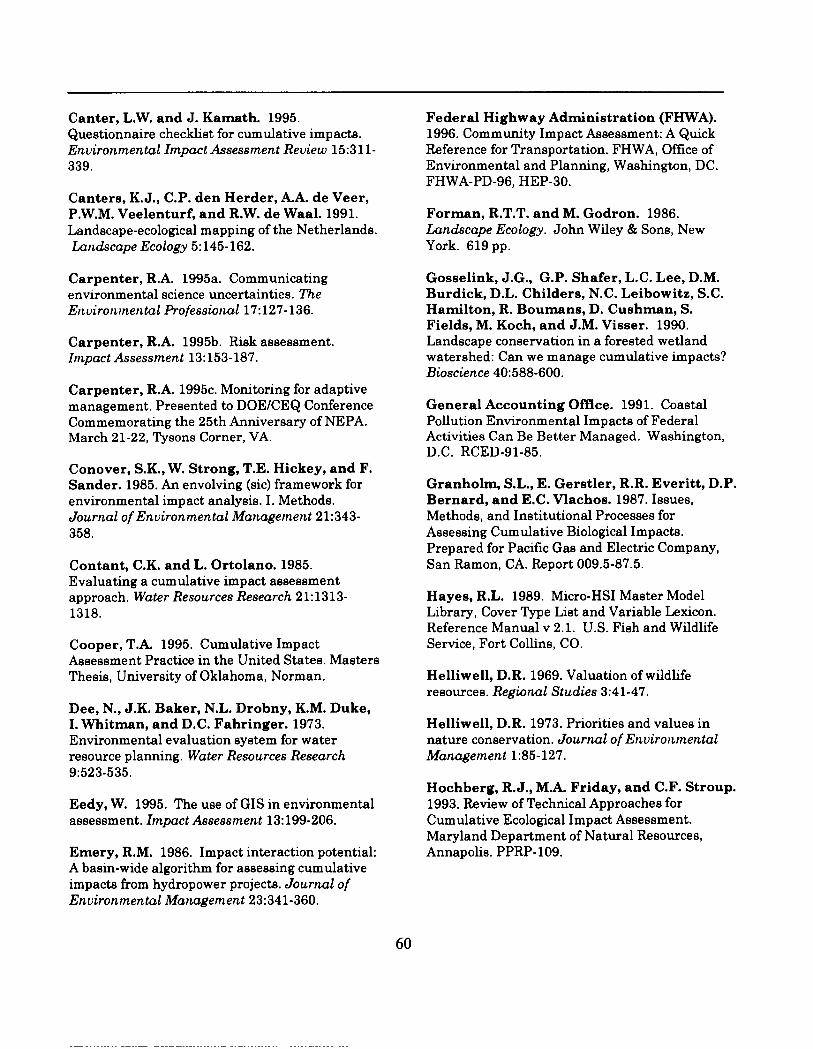
Canter, L.W. and J. Kamath. 1995.Questionnaire checklist for cumulative impacts.Environmental Impact Assessment Review 15:311-339.

Canters, K.J., C.P. den Herder, A.A. de Veer,P.W.M. Veelenturf, and R.W. de Waal. 1991.Landscape-ecological mapping of the Netherlands.Landscape Ecology 5:145-162.

Carpenter, R.A, 1995a. Communicatingenvironmental science uncertainties. TheEnvironmental Professional 17:127-136.

Carpenter, R.A. 1995b. Risk assessment.Impact Assessment 13:153-187.

Carpenter, R.A. 1995c. Monitoring for adaptivemanagement. Presented to DOE/CEQ ConferenceCommemorating the 25th Anniversary of NEPA.March 21-22, Tysons Corner, VA.

Conover, S.K., W. Strong, T.E. Hickey, and F.Sander. 1985. An envolving (sic) framework forenvironmental impact analysis. I. Methods.Journal of Environmental Management 21:343-358.

Contant, C.K. and L. Ortolano. 1985.Evaluating a cumulative impact assessmentapproach. Water Resources Research 21:1313-1318.

Cooper, T.A. 1995. Cumulative ImpactAssessment Practice in the United States. MastersThesis, University of Oklahoma, Norman.

Dee, N., J.K. Baker, N.L. Drobny, K.M. Duke,I. Whitman, and D.C. Fahringer. 1973.Environmental evaluation system for waterresource planning. Water Resources Research9:523-535.

Eedy, W. 1995. The use of GIS in environmentalassessment. Impact Assessment 13:199-206.

Emery, R.M. 1986. Impact interaction potential:A basin-wide algorithm for assessing cumulativeimpacts from hydropower projects. Journal ofEnvironmental Management 23:341-360.

Federal Highway Administration (FHWA).1996. Community Impact Assessment: A QuickReference for Transportation. FHWA, OffIce ofEnvironmental and Planning, Washington, DC.FHWA-PD-96, HEP-30.

Forman, R.T.T. and M. Godron. 1986.Landscape Ecology. John Wiley & Sons, NewYork. 619 pp.

Gosselink, J. G., G.P. Shafer, L.C. Lee, D.M.Burdick, D.L. Childers, N.C. Leibowitz, S.C.Hamilton, R. Boumans, D. Cushman, S.Fields, M. Koch, and J.M. Visser. 1990.Landscape conservation in a forested wetlandwatershed: Can we manage cumulative impacts?Bioscience 40:588-600.

General Accounting OffIce. 1991. CoastalPollution Environmental Impacts of FederalActivities Can Be Better Managed. Washington,D.C. RCED-91-85.

Granholm S.L., E. Gerstler, R.R. Everitt, D.P.Bernard, and E.C. Vlachos. 1987. Issues,Methods, and Institutional Processes forAssessing Cumulative Biological Impacts.Prepared for Pacii3c Gas and Electric Company,San Ramon, CA. Report 009.5-87.5.

Hayes, R.L. 1989. Micro-HSI Master ModelLibrary, Cover Type List and Variable Lexicon.Reference Manual v 2.1. U.S. Fish and WildlifeService, Fort Collins, CO.

Helliwell, D.R. 1969. Valuation of wildliferesources. Regional Studies 3:41-47.

Helliwell, D.R. 1973. Priorities and values innature conservation. Journal of EnvironmentalManagement 1:85-127.

Hochberg, R. J., M.A. Friday, and C.F. Stroup.1993. Review of Technical Approaches forCumulative Ecological Impact Assessment.Maryland Department of Natural Resources,Annapolis. PPRP-109.

60

Horak, G. C., E.C, Vlachos, and E.W. Cline.1983. Methodological Guidance for AssessingCumulative Impacts on Fish and Wildlife. Reportto U.S. Fish and Wildlife Service. DynamacCorporation, Fort Collins, CO.

Hubbard, P. 1990. Cumulative EffectsAssessment and Regional Planning in SouthernOntario. Canadian Environmental AssessmentResearch Council, Hull, Quebec. 45 pp.

Hunsaker, C.T. and D.E. Carpenter. 1990.Environmental Monitoring and AssessmentProgram —Ecological Indicators. U.S.Environmental Protection Agency, ResearchTriangle Park, NC. EPA 600/3/-89/060.

Hunsaker, C.T., R.L. Graharq G.W. Suter II,R.V. O’Neill, L.W, Barnthouse, and R.H.Gardner. 1990. Assessing ecological risk on aregional scale. Environmental Management14:325-332.

Interagency Ecosystem Management TaskForce (IEMTF). 1995. The Ecosystem Approach:Healthy Ecosystems and Sustainable Economies,Vol. 10verview. Washington, DC.

Irwin, F. and B. Rodes. 1992. Making Decisionson Cumulative Environmental Impacts: AConceptual Framework. World Wildlife Fund,Washingtm, DC. 54 pp.

Jenkins, R.E. 1988. Information managementfor the conservation of biodiversity. In Wilson,E.O., ed. Biodiuersity. National Academy Press,Washington, D.C. pp 231-239.

Johnston, C.A., N.E. Detenbeck, J.P. Bonde,and G.J, Niemi. 1988. Geographic informationsystems for cumulative impact assessment.American Society of Photogrammetry and RemoteSensing 54(11): 1609-1615.

Karr, J,R. 1991. Biological integrity: A long-neglected aspect of water resource management.Ecological Applications 1:66-84.

Karr, J. R., K.D. Fausch, P.L. Angermeier,P.R. Yant, and I.J. Schlosser. 1986. AssessingBiological Integrity in Running Waters: A Methodand Its Rationale. Illinois Natural History SurveySpecial Publication 5, Champaign, IL.

Lackawanna County Regional PlanningCommission. 1996. Lackawanna Valley CorridorPlan. Scranton, PA.

Lane, P.A. and R.R. Wallace. 1988. A User’sGuide to Cumulative Effects Assessment inCanada. Canadian Environmental AssessmentResearch Council, Ottawa, Ontario.

Larsen, D.P, and S.J. Christie. 1993. EMAP-Surface Waters 1991 Pilot Report. U.S.Environmental Protection Agency, Corvallis, OR.EPM620/R-93/003.

Leibowitz, S.G., B. Abbruzzese, P. Adamus, L.Hughes, and J. Irish. 1992. A SynopticApproach to Cumulative Impact Assessment—AProposed Methodology. U.S. EnvironmentalProtection Agency, Corvallis, OR. EPM600/R-92/167.

Lewis, T.E. and B.L. Conkling, eds. 1994.Forest Health Monitoring Southeast Loblolly/Shortleaf Pine Demonstration Interim Report.U.S. Environmental Protection Agency,Washington, DC. EPA/620/R-94/006.

Marlatt, R.M., T.A. Hale, and R.G, Sullivan.1993. Video simulation as a part of Armyenvironmental decision-making: Observationsfrom Camp Shelby, Mississippi. EnvironmentalImpact Assessment Review 13:75-88.

McCabe, G,, C. Orians, C. Clavate, and K.Branch. 1991. Driving variables that impactenvironmental quality. Battelle Pactilc NorthwestNational Laboratory, Richland, WA.

McCold, L, and J. Holrnan, 1995. Cumulativeimpacts in environmental assessments: How wellare they considered. The EnvironmentalProfessional 17:2-8

61

McHarg. I. 1969. Design with Nature. NaturalHistory Press, New York, NY. 197 pp.

Messer, J. J., R.A. Linthurst, and W.S.Overton. 1991. An EPA program for monitoringecological status and trends. EnvironmentalManagement 17:67-78.

National Academy of Sciences. 1993. ABiological Survey for the Nation. NationalAcademy Press, Washington, DC.

National Park Service. 1990. FinalEnvironmental Impact Statement. Mining inYukon- Charles Rivers National Preserve, Alaska.Cumulative Impacts of Mining. Volume 1.Anchorage, AK.

National Performance Review. 1994.Creating a Government that Works Better andCosts Less. Washington, D.C. September.

National Research Council (NRC). 1986. Thespecial problem of cumulative effects. InCommittee on the Applications of EcologicalTheory to Environmental Problems. EcologicalKnowledge and Problem Solving: Concepts areCase Studies. National Academy Press,Washington, D.C. pp. 93-103.

Nestler, J. 1992. Cumulative impact assessmentin wetlands. Wetlands Research Program Bulletin1:1-8. U.S. Army Corps of Engineers, Vicksburg,MS.

Ness, R,F 1990. Indicators for monitoringbiodiversity: A hierarchical approach.Conservation Biology 4:355-364.

Odum W.E. 1982. Environmental degradationand the tyranny of small decisions. Bioscience33:728-729.

O’Neill, R.V., J.R. Krummel, R.H. Gardner, G.Sugihara, B. Jackson, D.L. DeAngellis, B.T.Milne, M.G. Turner, B. Zygmunt, S.W.Christensen, V.H. Dale, and R,I. Graham.1988. Indices of landscape pattern. LandscapeEcology 1:153-162.

O’Neill, R.V., K.B. Jones, K.H. Riiters, J.D.Wickha~ and LA. Goodman. 1994. LandscapeMonitoring and Assessment Research Plan. U.S.Environmental Protection Agency, Las Vegas, NV.EPA/620/R-94/009.

Overton, W.S., D. White, and D.L. Stevens.1990. Design Report for EMAP (EnvironmentalMonitoring and Assessment Program). U.S.Environmental Protection Agency, Corvallis, OR.EPA/600/391/053.

Patterson, N.J. and T.H. Whillans. 1984.Human interference with natural water levelregimes in the context of other cultural stresses onGreat Lakes wetlands. In H.H. Prince and F.M.D’Itri, eds. Coastal Wetlands. Lewis Publishers,Inc., Chelsea, MI.

Peterson, E.B., Y.H. Chan, N.M. Peterson,GA. Constable, R.B. Caton, C.S. Davis, R.R.Wallace, and G.A. Yarranton. 1987.Cumulative Effects Assessment in Canada: AnAgenda for Action and Research. CanadianEnvironmental Assessment Research Council,Hull, Quebec.

President’s Council on Sustainable Develop-ment. 1996. Sustainable America: A NewConsensus for Prosperity, Opportunity, and aHealthy Environment in the Future, Washington,DC. 186 pp.

Preston, E.M., and B.L. Bedford. 1988.Evaluating cumulative effects on wetlandfunctions: A conceptual overview and genericframework. Environmental Management 12:565-583.

62

Radbruch-Hall, D.H., K. Edwards, and R.M.Batson. 1987. Experimental Engineering-Geologic and Environmental-geologic Maps of theConterminous United States. Bulletin 1610. U.S.Geological Survey, Reston, VA.

Ranasinghe, J.A., S.B. Weisberg, J. Gerritsen,and D.M. Dauer. 1994. Assessment ofChesapeake Bay Benthic MacroinvertebrateResource Condition in Relation to Water Qualityand Watershed Stressors. Prepared for TheGovernor’s Council on Chesapeake Bay ResearchFund and Maryland Department of NaturalResources, Annapolis, MD.

Reid, W.V., J.A, McNeely, D.B, Tunstall, andD. Bryant. 1991. Indicators of BiodiversityConservation. World Resources Institute,Washington, D.C.

Risser, P., J.R. Karr, and R.T.T. Forman.1984. Landscape Ecology: Directions andApproaches. Champaign: Illinois Natural HistorySurvey, Special Publication 2.

Schamberger, M., A.H. Farmer, and J.W.Terrell. 1982. Habitat Suitability Index Models:Introduction. U.S. Fish and Wildlife Service,Washington, D.C.

Sutherland, M.T. and J.B. Stribling. 1995.Status of biological criteria development andimplementation. In Davis, W. and T. Simon, eds.Biological Assessment and Criteria: Tools forWater Resources Planning and Deciswn Making.Lewis Publishers, Inc, Chelsea, MI. pp. 79-94.

Sutherland, M.T. and S.B. Weisberg. 1995.Maryland Biological Stream Survey: The 1995Workshop Summary. Chesapeake Bay Researchand Monitoring Division, Maryland Department ofNatural Resources, Annapolis. CBRM-BA-95-2.

Spaling, H. 1995. Cumulative effectsassessment. Impact Assessment 12:231-251.

Spaling, H. and B. Smit. 1993. Cumulativeentionmental change: conceptual frameworks,evaluation approaches, and institutionalPerspectives. Environmental Management17:587-600.

Stakhiv. E.Z. 1988. An evaluation paradigm forcumulative impact analysis. EnvironmentalManagement 12:725-748.

Stakhiv, E.Z. 1991. A cumulative impactanalysis framework for the US Army Corps ofEngineers regulatory program. Draft report(February 1991). Institute for Water Resources,US Army Corps of Engineers, Fort Belvoir, VA.282 pp.

Stowell, R., Espinosa, T.C. Bjornn, W.S.Platts, D.C. Burns, and J.S. Irving. 1983.Guide for Predicting Salmonid Response toSediment Yields in Idaho Batholith Watersheds.U.S. Forest Service, Northern and IntermountainRegions.

Stun, E.A., K.E, LaGory, and W.S. Vinikour.1987. Methodologies for Assessing theCumulative Environmental Effects ofHydroelectric Development on Fish and Wildlifein the Columbia River Basin Volume 1:Recommendations. Final report to BonnevillePower Administration, Portland, OR. DOE/BP-19461-3.

Summers, J. K., J.M. Macauley, V.D. Engle,G.T. Brooks, P.T. Heitmuller, A.M. Adams.1993. Louisiana Province Demonstration Report:EMAP —Estuaries, 1991. U.S. EnvironmentalProtection Agency, Gulf Breeze, FL. EPM620/R-94/001

Suter, G.W, IL 1993. Ecological RiskAssessment. Lewis Publishers, Boca Raton, FL.

Thornton, K. W., G. E. Saul, and D. E. Hyatt.1994, Environmental Monitoring and AssessmentProgram Assessment Framework. U.S.Environmental Protection Agency, ResearchTriangle Park, NC. EPA/620/R-94/O16.

63

U.S. Army Corps of Engineers (USACE). 1980.A Habitat Evaluation System for Water ResourcePlanning. U.S. Army Corps of Engineers,Vicksburg, MS. 88 pp.

U.S. Army Corps of Engineers (USACE),Washington Department of Ecology, and Port ofSeattle. 1994. Southwest Harbor Cleanup andRedevelopment Project: Joint Federal/state DraftEnvironmental Impact Statement. Seattle, WA.

U.S. Bureau of Land Management ( BLM).1990. Final Environmental Impact Statement.Castle Mountain Project, San Bernadino County,California. Needles, CA.

U.S. Environmental Protection Agency. 1992.Framework for Ecological Risk Assessment. RiskAssessment Forum, Washington, DC. EPA 630/R-92-001.

U.S. Environmental Protection Agency. 1993.A Guidebook to Comparing Risks and SettingEnvironmental Priorities. Washington, DC. EPA230-B-93 -O03.

U.S. Forest Service. 1993. Pacific Yew FinalEnvironmental Impact Statement. USDA, ForestService, Paciilc Northwest Regional Office,Portland, OR.

U.S. Fish and Wildlife Service. 1980. HabitatEvaluation Procedures. ESM 102. US Fish andWildlife Service, Division of Ecological Services.Washington, D.C.

Vestal, B., A, Rieser M. Ludwig, J. Kurland,C. Collins, and J. Ortiz. 1995. Methodologiesand Mechanisms for Management of CumulativeCoastal Environmental Impacts. Part I—Synthesis, with Annotated Bibliography; Part H-Development and Application of a CumulativeImpacts Assessment Protocol. NOAA CoastalOcean Program Decision Analysis Series No. 6.NOM Coastal Ocean Office, Silver Spring, MD.

Weisberg, S.B., J.B. Frithsen, A.F. Holland,J.F. Paul, K.J. Scott, J.K. Summers, H.T.Wilson, R. Valente, D.G. Heimbuch, J.Gerritsen, S. C Schimmel, and R.W. Latimer.1993. EMAP-Estuaries Virginian Province 1990Demonstration Project Report. USEPA,Environmental Research Laboratory,Narragansett, RI. EPA 600/R-92/100.

Westman, W.E. 1985. Ecology, ImpactAssessment, and Environmental Planning. Wiley-Interscience, New York, NY.

Williamson, S.C, 1993. Cumulative impactsassessment and management planning: Lessonslearned to date. In Hildebrand, S.G. and J.B.Cannon, eds. Environmental Analysis: The NEPAExperience. Lewis Publishers, Boca Raton, FL. pp391-407.

Williamson, S.C. and K. Hamilton. 1989.Annotated Bibliography of Ecological CumulativeImpacts Assessment. U.S. Fish and WildlifeService Biological Report 89(11). National EcologyResearch Center, Fort Collins, CO.

Witmer, G., J.S. Irving, and M. Bain. 1985. AReview and Evaluation of Cumulative ImpactAssessment Techniques and Methodologies.Prepared by kgonne National Laboratory forBonneville Power Administration.

World Commission on Environment andDevelopment. 1987. Our Common Future.Oxford University Press, UK.

64

A-1

APPENDIX A

SUMMARIES OFCUMULATIVE EFFECTS ANALYSIS METHODS

A-2

METHODS

A-3

1QUESTIONS, INTERVIEWS, AND PANELS

��

��

��

��

��

��

��

��

��

��

��

!��

��

�� "��

� �� #$�� %&'() ��

��

��

�� *�� +��

�� ,�� -� ��

��, #�� #.�� %&&/0 1��

� � � �� )� *�� %&2')� 3��

��

��

�� -��

�� -� ��

�� #�� %&2')�

�� -� �� -��

��

METHODS

A-4

1EXAMPLES:

�� 4�� #�� ) �� 5�

��

��

�� 6�� 3��

�� ,*�� +��, ��

�� 763 #689� ��

�� "�� :�� %&&;� %&&<)� ��

�� 6�� :�� =��

�� -� �� >�� *�� 3�� #689�

?�� $�� =�� #%&&@) �� *�� 9�� %&&<) ��

��

�� *�� 3��

�� #:�� <� �� <�

%)� +� �� ;A ��

��

�� %; �� #��

� ��) � ��

��

��

��

��

��

��

�� *�� 3�� 6�� 8�� 9��

��

��

��

��

��

*�� 3��

��

��

�� 7��

�� *��

��

� � � � � � � � � � � � �

References

6�� 8�� 9�� #689�) *��

9�� %&&<� 6�� 8�� 9�� *��

3�� 3��

:�� B� ��

6�� 8�� 9�� #689�) �� :��

%&&;� 6�� 8�� 9�� *��

8�� C *�� +��

B� ��

6�� 8�� 9�� #689�) �� :��

%&&<� 6�� 8�� 9��

� �� B� +��

.�� .�D�� *�"� 1�� 8� � .�� "��

"�8�� %&&/� ��

�� C �� E�� ?�� $��

=� ��

%2#;)C;&(�<@A�

$�� .� � �� =� �� %&'(� ��

��

��1�� 3�� :�� *�� = �

METHODS

A-5

�� 6� �� B�6� $�E�� 1�� 8�� 1�� *� �� F� *�� %&2'� ��

%&2'� =��

��

�� :�� ;(C%A'�%2@�

*�� ?�� 8�� %C *� ��

"96G?3�%&/A%�<� +�� ?��

3�� 3�� 9*�

>�� ?�� $�� =�� %&&@� +��

6�� :��

=�� 3�-� �� ?�� :��

:�� 7�� : �

METHODS

A-6

2CHECKLISTS

��

�� ,�� , ��

�� :��

��

�� =��

��

�� -� �� :��

:��

��

� ��

��

��

��-� �� 0 ��

�� -� ��

�� ?� �� #��

�� ) � ��

��

�� #��

�� =�� <)� ��

�� 0

��

��

��

METHODS

A-7

2EXAMPLES:

�� -� �� ,"�� , ��

�� #��

�-� �� #:�� %&&A)�

�� )� ��

��

6�� 6 � #�� >�� "96 %&&/)� �� >�� :��

:�� "�� #%&&<) 6�� $�� #$�� %&'/)� ��

�� (A ��

�� -� �� & �� %%

!�� (( �� #D��

�� C B�� %&'<)� ��

Does the project have environ-mental effects which are individ-ually limited, but cumulativelyconsiderable? Cumulatively cons-iderable means that theincremental effects of an individualproject are considerable whenviewed in connection with theeffects of past projects, the effectsof other current projects, and theeffects of probable future projects.It includes the effects of otherprojects which interact with thisproject and, together, are consid-erable.

�� ,��, ��

� ��

��

�� :��

�� B�� #%&&() ��

��

��

��

�� ;�@@@ �� %�@@@

��

� ��

��

�� $�� #%&'%)�

:��

��

�� ,��, � ,�� , ,��, � ,��

��, �� ,� �� , � ,�� , ��

�� %

��

��

��

��

��

�� =��

��

��

METHODS

A-8

Table A-1. H ypothetical checklist for identif ying potential cumulative effects of a hi ghway pro ject

Potential ImpactArea

Proposed Action OtherPast Present Future Cumulative

Actions Actions Actions ImpactConstruction Operation Miti gation

Topography and ** * **Soils

Water Quality ** * + * * * ***

Air Quality ** * **

Aquatic ** ** + * * **Resources

Terrestrial * * * **Resources

Land Use * *** * * ***

Aesthetics ** *** + * **

Public Services * + + +

Community * * *Structure

Others

KEY: * low adverse effect ** moderate adverse effect *** high adverse effect+ beneficial effect � no effect

References

:�� "�� *��

#:��)� %&&<� 6�� 6�<'� >�� :�� 6��

:�� :�� :�� 7� @26/;(� 3�-� � $�� :�� $�

*�� 6�� " ��

�� ;%( �� %@ � �* <@� & � $�� $�?�� +�6� :�� ?�?� .��

:�� $�1� %&&A� �� 6�� :�� A/(� >��

��! "�� = E��.�� 7�� E�� %< �

F��

:�� $�1� �� D� B�� %&&(� !�� 6�� :�� 9��

�� 763 9�� >�� "96� 1�� ":�

�� #��

%(C<%%�<<&�

D�� *�B� �� *� B�� %&'<� 6��

��

�� *�� "�%<� >��

:�� 6�� $��

:�� $�

$�� 6�F�� %&'/� 6��

D�*� ?�� %&'%� 3� �� 6��

>�� "�� 6�� #"96)� %&&/�

METHODS

A-9

3MATRICES

��

�� #��

�� )� ��

��

��

��

�� #$�� %&'%) �� 4

��

�� #?�� %&2A0 ��

�� %&2'0 $�E�� %&&<)� ��

=�� #��

�� G� ��G ��)� � ��

��

�� -� �� 9� � ��

��

��

�� $�� -� �� 1��

��% ��

�� & ��' ��

�� ! =��

��

��

��

�� =��

� ��

�� #:�� %&&A)� ��

��

�� +� �� %

� ��

�� #�� ?� ��

�� )� ��

�� 0 �� #��

�� =�� /)�

� ��

� ��

METHODS

A-10

3EXAMPLES:

=��

�� >�� -� ��

E�� #$�� %&'%)� �� -� �� =��

�� :� 3 � ��

�� 9�� *�� *�� 6��

�� :�� #+6*:

�� 3� �� #:� 3) �� %&2A�� %&2'0 �� ?�� %&&<)� 9��

+�� 6�� *�� :��

��%&2@� #+6*: %&2(� %&2A�0 *�� %&2()� �� #?��

�� %&2A0 �� %&2'0 $�E�� %&&<)�

�� 6� � ��

��

�� :� 3 �� #�� 0 ��

��) �� #� � ��

� �� % � () �� -� � ��

�� #��

�� )� 6� � �� =�� #��

�� %&2'0 $�E�� %&&<) ��

�� ?�� #%&2A) ��

�-� � #+�� %)� � �� #�� )

��

�� -� � � ��

�� :� 3 �� -� ��

��

�-� ��

� �� 0 �� -� ��

�� +� ��

��

��

1�� #>�+1� %&2@0 ?�� %&2;)� � ��

��

��

METHODS

A-11

Figure A-1. Example of cumulative impact computations for a target resource with three resource componentsand two projects (FERC 1987).

References

?�� =�?�� D�� *�"� 9�� 6� � �� :�� $�1� %&&A� ��

�� E�1� 1�� %&2A� :�� & "�� = E��.�� 7��

��C �� F��

��

7$G66��=�<@&� �� 7�� +�� 6�� *�� :�� #+6*:)�

$�� $� %&2(� 3� ��

?�� B�"� %&2;� �� (�� #�� (@C<<2(�</@<�

��

�� +�� 3�� +�� 6�� *�� :�� #+6*:)�

%;� +1�G9?��2;G;A� >�� +�� 1�� %&2A�� 9�� *�� ?��

�� 1�� 6�� $�� >�� -� �� :�� +�� 6�� *��

+�� :�� :9� :�� 1�� "�:� +6*:G"6��

�-� �� C ��

@@/%�

METHODS

A-12

+�� 6�� *�� :�� #+6*:)� $�� $�?�� +�6� :�� ?�?� .��

%&2A�� *�� ?�� D�*� ?�� %&'%� 3� �� 6��

�� -� �� 1�� +�� 6�� :�� A/(� >��

6�� *�� :�� 1�� E�� %< �

"�:� +6*:G+6��@@/;�

+�� 6�� *�� :�� #+6*:)� ��

%&2'� �� *�� ?�� 3 </A�<(@ �� +�1� 9�� *�E�

�-� �� +�� 6�� *�� 1�� *�.� .�� #��)� 3� ��

:�� 1�� "�:� +6*:G+6�� .�� +��

@@//� �� +�� ?�� ="�

�� D�� =�?� ?�� %&&<� �� 6� �� B�6� $�E�� 1�� 8��

:�� +�� 1�� %&2'� =��

�� *�� ?�� E� .��

�� D�?� :��

�� )�*� �� $�� 3�� ? � �� :�� *�� ?�� H 8�� ;C 6��

*�� +$� � <('�<';� �� +��

$�E�� B�6�� 6� � �� 1�� 8�� "96G?3�%&/A%�/�

%&&<� 3��

�� >�� +�� 1�� %&2@� .��

�� :�� *�� ?�� 3� /@2�/;< �� 6�= %@;� >�� +��

��E� .�� D�?� :�� 1�� "�� 6 ��

�� )�*� �� 1�� "�:�

$�� 3�� ? � *�� +$�

*�� 7� %&2(� 3��

?�� 3�� 3�� 9*�

METHODS

A-13

4NETWORKS AND SYSTEM DIAGRAMS

�� 4 ?� ��

�� #��)� ��

�� #��) � �� #� � ��

��) � ��

�� 7��

��

��

��

��

� �� #�� ) ��

��

�� 7��

�� +� �� 5�

�� '��'��

�� ! ��

7�� #E�� *�� %&'')�

��

�� 6��

�� 6��

�� #� ��) � ��

�� #�� )� ��

7�� #%) ��

��

�� :�� #;) ��

��

��

�� #��

�� )� 1�� 5�

��

��

�� #��

��)� ��

��

��

��

#�� )�

��

METHODS

A-14

Figure A-2. Example of an “impact tree” for new freeway construction in an established downtown businessdistrict (modified from Rau and Wooten 1985)

4EXAMPLES:

�� #:��) 6��

�� #%&'%)� �� 3�� #%&&/)�

��

��

�� +��

�; ��

� �� +�� / #?�� %&2<)� ��

�� #�� *�� 1�� %&2() ��

��

�� #�� ) ��

�� $� ��

��

�� #+�� <) ��

�� 0 ��

��

��

METHODS

A-15

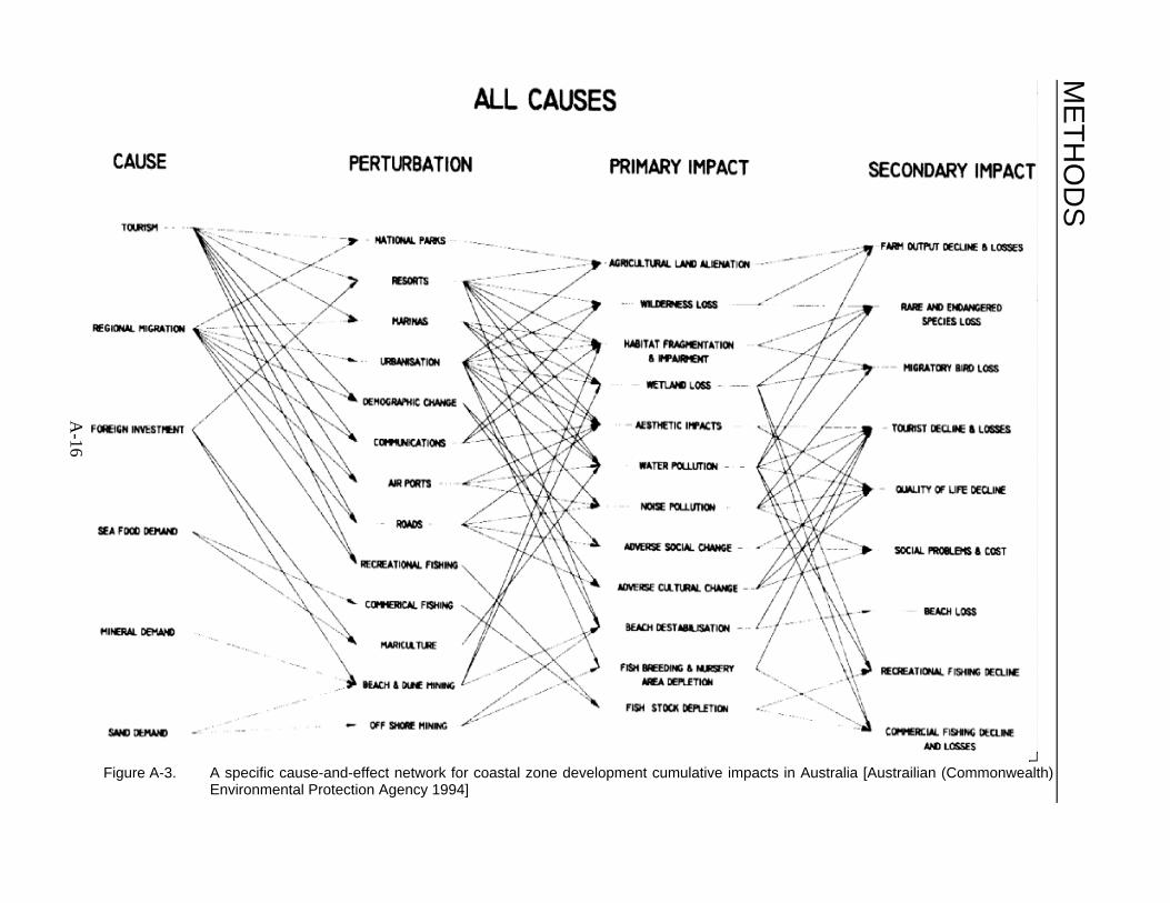
ME

TH

OD

S

A-16

Figure A-3. A specific cause-and-effect network for coastal zone development cumulative impacts in Australia [Austrailian (Commonwealth)Environmental Protection Agency 1994]

METHODS

A-17

Figure A-4. System diagram showing cumulative indirect effects of aerial application of herbicide on an aquaticsystem (Bisset 1983).

� �� :�� ?�� *��

3��

��

�� ?��

#1�� %&2')� ��

��

� �� #�� ) �

�� #��

��) � � ��

��

�� ?��5� ��

��

� ��

��

�� #1�� %&&<)�

References

�� #:��) 6��

3�� %&&/� ��

:��

6�� :��

*�� =��

?�� *� %&2<� =��

�� C ��

��

�� %%C;'�/<�

E��=�1� �� 3�E� *�� %&''� ��

��

�� <C%22�;@&�

*�� D�E� �� "�:�1�� %&2(�

�� ,��-�

= E��.�� 7�� F��

METHODS

A-18

�� D�:� %&'%�� (�� - �� 1�� :�� :�$� �� E�1� B�� $�

�� .�� #��

�� .�� /��

�� .�� 0�� >�� :��

?�� : �

1�� :� %&&<� :��

�� C $��

$�� "�� C ��E� .�� D�?�

:�� #��)��

)�*� �� $�� 3�� ? � *��

+$� � <&%�/@'�

+�� 7� .�� %&2'� :��

�� C � ��

:�� ?�� )��

�� 1�� )�� #��

.�� (;C<''�<22�

METHODS

A-19

5MODELING

�� ' ��

�� '��'�� C

�� =��

��

� �� .��

�� 9��

�� -� � � ��

�� =��

� ��

�� *��

�� #�� =�� %@ �� %%)�

"�� -� ��

�� +� ��

�� 763 � ��

��

� �-� �� *��

�� 7��

��

��

�� #%) ��

�� #;) �� 7��

��

��

�� E��

��

��

� � � � � 6 � ��

=��

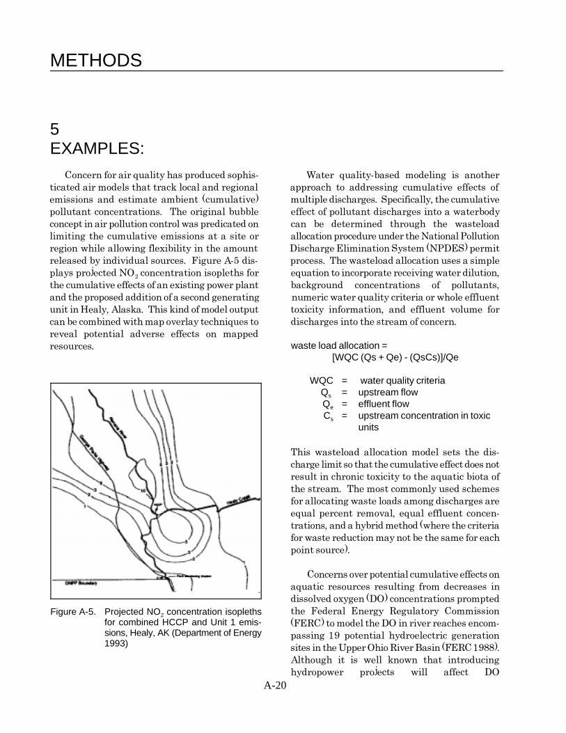
METHODS

A-20

Figure A-5. Projected NO concentration isopleths2

for combined HCCP and Unit 1 emis-sions, Healy, AK (Department of Energy1993)

5EXAMPLES:

:� �� 1��

��

�� # ��) ��

��

� ��

�� 7�� 3��

�� "�� 6�� #73"6�) ��

�� +�� ( ��

�� -� �� 79 � �� ;

��

��

�� .��

��

��

�� waste load allocation =[WQC (Qs + Qe) - (QsCs)]/Qe

WQC = water quality criteriaQ = upstream flows

Q = effluent flowe

C = upstream concentration in toxics

units

��

��

��

��

��

��

�� #��

��

�� )�

:� ��

��

�� #"9) � ��

�� +�� 6�� *�� :��

#+6*:) �� "9 ��

�� %& ��

�� >��9��*��?�� #+6*:%&22)�

��

�� -� �� "9

METHODS

A-21

Figure A-6. Cumulative effects on dissolved oxygencaused by hydroelectric development,reduced spillages, and reduced aera-tion at dams (FERC 1988)

� ��

�� #��

�� )� ��

��

�� #+�� A)�

��

��

�� "9 ��

�� "9 ��

��

� � ��

��

�� #?9") ��

��

��

�� "9 � ��

�� >��

�� -� �� "9 � ��

��

��

# �� -� ��) � ��

��

��

��

�� #��

�� ) � ��

��

�� .�� 6�� 3� �� #.630>�� +��

�� *�� =�� 1�� %&2@) �� +��

�� =�� #�+�=0 ��

� �� #$�� 6�� %&2()� �� %&2/) �� >�� +�� 1��

�� .63 �� .��

�� #.��) ��

� �� #� �� %&2;0 .�� %&2&)�

�� .��

��

��

�� ?�� .��

� ��

�� / � ;@�� #� �� %&2A)� ��

�� -� �� 1��

�� 'I �� -��

�� # �� .��

�� 0 %<I � ;/I �� ) �� .63 ��

�� -� � �� +�=�� #��

�� #%&&/) � �� ) ��

��

METHODS

A-22

=��

� �� 1��

� �� 763 ��

�� >�� 6 ��

�� +�� #6�+�) ��

#%)�� #;)��

�� #<) ��

�� 6�+� ��

�� 6 ��

#=�� %@)�

��

��

��

��

��

9�� #��

��) ��

��

�� -� �

�-� �� =��

��

��

��

�� #�� %&2')�

E�� #%&2() ��

� ��

��

��

��

��

��

�� #��

�� ) ��

��

��

��

�� J�

��

References

�� :�$�� *�D� +�� D�1� �� %&2/

:�� >�� .�� 6��

3� �� #.63) �� +��

�� =�� #�+�=) ��

�� >�� +�� 1��

1�� 6�� $��>�� +��

:�� :9� +1�G9?��2/G%%�

+�� 6�� *�� :�� #+6*:)�

%&22� +�� 6��

.�� "�� >�� 9��

*�� ?�� 9�� 3��1�� 8��

+6*:" �� 7� 6$2(�%&�%%/� +�� 6��

*�� :�� 9�� .��

$� ��1�� ":� ��

+6*:G+6��@@(%�

E�� D�:� �� D�*� �� %&2(�

��

��1�� #�� #�� %AC%/�

;@�

.�� *�$� %&2&� =� ��.��

��

*�� =�� ;�%� >�� +�� 1��

�� +�� :�� :9�

$�� =�"� 6�� %&2(� :��

6�� =� ��.��"��

+�� *�� "��=��

�C �� *�� 3�� ?��

3�� 3�� 9*� %%/ � K

��

� ��=�� .� +�� D�1� ��

%&2;� .�� =��C

�� >�� +�� 1��

1�� ":�

� �� *�$� %&2A� .��

=��C1�� *� ��

�� ?�� *�� 2;#%@�%;2)� >��

+�� 1�� 1�� ":� %'

�

METHODS

A-23

�� 6� �� B�6� $�E�� 1�� 8�� >�� "�� 6�� %&&<� +��

%&2'� =�� 6��

�� 3��.�� :�� :�� 3�-� �� "96G6��

�� :�� @%2A�

*�� ?�� H 8�� ;C 6��

�� +�� ?�� 3�� >�� +�� 1�� %&2@� .��

�� 3�� 9*� "96G?3�%&/A%�/� 6�� 3� �� 6�= %@;� >�� +��

�� D�:�� .�$� �� :�1�� 1�� "�� 6 ��

%&&/� 6 �� C �� 1�� ":�

?�� #��

�� (� 1�� ,��! ��

1�� ?��=" � A@'�A;;�

METHODS

A-24

6TRENDS ANALYSIS

��

��

��

�-� �� :��

��

��

��

��

��

��

� ��

�� 1��

��

��

� ��

�� +�

��

��

��

� ��

�� 1��

�� #�

� ��)� ��

��

��

��

��

��

� !�"��

��

��

:��

��

�� .��

��

��

��

?��

��

��

�� #��

�� )� ��

��

�� #��

�� )� :��

� ��

��

��

��

:��

�� <��

��

� �� 8��

��

��

��

��

�� >��

METHODS

A-25

Figure A-7. Common flicker population trends (Robbins et al. 1986)

6EXAMPLES:

��

��

�� +� ��

�� >�� +�� 1�� 5� ��

?�� ?�� #??�) �� #+�� ')� ��

��

�� #*��

%&2A)� � �� # ��

�� ??� �� %&&@0 �� %&&;)�

METHODS

A-26

Figure A-8. Cadiz township forest fragmentation(Curtis 1956 cited in Terborgh 1989)

�� =��

�� >�� +��

� �� +�� 2 1�� 5� 7�� 1��

�� #71�0"�� %&&%)� ��

�� 1�� #:�� #�� ) ��

%&(A �� %&2&)� �� 71� ��

��>�� :�� 6�� #��

�� >�� 63 � +�� 1�� ) ��

79 #%&&<)� ��

�� :�� ?��

1 � �� ,�� , � ��

� �� %2''� � �� >�� 63

%/@ �� 6��*�� $�� :��

�� #$�� %&&;) ��

��

��

��

��

��

��

�� #�� ;)� ��

4 ��

�� +�

��

��

� ��

�� $��

� ��

��

��

��

��

��

��

��

��

�� 6�� : � �� (@�

��

�� #"� ��

�� %&2()� ��

��

��

METHODS

A-27

Table A-2. Habitat loss b y historic period in Commencement Ba y, WA(modified from USACE 1993)

Historic Period Habitat Type of Lost Habitat photo graphic evidence)Historical Records historical records and Acres Remainin g

Total Lost Habitat (includes

1877 - 1894 mudflat 11 0 2,074marsh 20 0 3,874

1894 - 1907 mudflat 208 605 1,469marsh 41 415 3,459

1907 - 1917 mudflat 51 542 927marsh 35 64 3,395

1917 - 1927 mudflat 48 162 765marsh 0 72 3,320

1927 - 1941 mudflat 143 133 632marsh 399 1,676 1,44

1941 - Present mudflat 105 412 187marsh 1,557 1,587 57

TOTALS mudflat 566 1,54marsh 1,052 3,814

References

�� *� �� D�+� $�� *� E�� $�� E�� ?� �� 3� �� $�

%&&@� 3�� .�� D� �� %&&;� ��

�� 7�� .�� 2�� 'C%� � :�� J 3��

('� =�� >�� 6�� 3��

:�� D�� %&(A� �� :�� 9*� 63 GA@@G*�&;G%A'�

�� +�

#�� .�� (�� & ��

1�$� �� ';%�'<A� >�� :��

3�� $�

"�� 6�� :�6� D�� 1�6� +�� %&&%�

1��C ��

:��>�� =��%&'@5� � =��

%&2@5�� >�� "�� +��

1�� 1�� ":� ;2 �

"� �� E� �� 6� �� %&2(� :��

�� C

��

�� #�� (C<'�

A/�

�� 6�� *�� $��

*�� :�� "� ?�� 3�.� E�� %&2A�

�� ?�� ?�� C �� +�� +��

F�� %&A(�%&'&� >�"9�� +�� 1��

�� *�� 3�� %('�1��

":�

�� D� %&2&�1�� ,�� 3��

4��5 3�� >�� 3�� 7D� ;@' �

�� D� %&&;�1��

8��"�� ;AA#()C&2�%@/�

>�� :�� 6�� #>� :6) � >��

+�� 1�� 79 � %&&<�

:�� ?�� :��

8�� >�� :��

6�� 1 �=��GD��

METHODS

A-28

7OVERLAY MAPPING AND GIS

#��

�� $%�&' �� #= .�� %&A&)�

��

�� *��

� ��

��

�� 9�� *��

�� 5� ��

�� =�� E��

�� #*�� %&2')� � � ��

�� #= B��

� �� =� �� %&'()� *��

�� ' ��

��! #*�� %&2')� 9��

��

�� ,�� , ��0 ��

��

��

�� 6��

��

� ��

��

��

��

��

� ��

��

,�� , �� #:��

�� 1�� %&&<)� 1��

�� #��

��) ��

��

�� *��

�� #��

�� ) � � � � � � � � � � � � � �

��

��

�� #�� )�

METHODS

A-29

9��

��

E�� #�� -� � � ��

�� ?�� %&22)� �� #�� )�

��

�� 6� � �� >�� E��

� ��

�� 1�� #� ��)� ��

�� #��) �� #D�� %&22)� ��

�� E��

��

�� $��

�� E��

��

�� #� ��

��) ��

��

� ��

��

METHODS

A-30

7EXAMPLES:

6�� ,�� , � ��

E��

�� #��

�� =��

�� ) ��

�� #��

� ��

�� )� ��

�� E��

��

��

�� =��

�� +� ��

�� 5� �� #��

�� +� �� ) ��

��

�� #��

�� # �� )� 9��

��) ��

�� :��

�� "�� 6��

�� :�� . ��

6��1�� 8�� #1�� 8��"9�%&&;)� #��

E��

�� ) �� #��

�� ) ��

��

�� "�� 7�� 7��

�� 3�� *�� ="� %&&A)�

�� #��

�� 9�� E��

� �� )� ��

�� 1�� )��& �� = .�� #%&A&) �� 1�� #%&2') ��

�� E��

��

�� 3�� 3�� ?�� 9�� +��

?�� #��

��

1�� "�:� ��

��

�� +�� & #��

METHODS

A-31

Figure A-9. Hypothetical intersection between aviation flight corridors and environmental resources near a typicalU.S. military installation (Department of the Navy 1996)

�� ) �� E��

��

�� E��

�� #�� %&&/) ��

�� #$�� = :�� %&&()� D��

9�� +�� #%&&/) �� E��

�� #��

�� ) �� .� �� E��

�� #%) ��

�� #;)�� #<) ��

�� #/) �� #() ��

� ��

METHODS

A-32

�� 3� �� 7��

��

E�� 9�� E��

�� #�

�� ) � �� 3��

��

��

��

� �� #��

�� )� 9�� E��

��

��

�� #�� :�� ) �

��

References

?�� *�E� %&22� 3��

��

��

�� %;C%%�%'�

:�� :�B� �� $�$�1�� %&&<� ��

"�� :�� C

3�� :�� C

��E� .�� D�?� :��

�� )�*� ��

$�� 3�� ? � *�� +$� � <<A�<(A�

"�� 7�� %&&A� .��

��

�� >��

�� =� �� D��

��

#D��) 3��9�� 7��

3�� *�� ="�

+�� D�+� %&&/� "��

��

�� C �� E�� C 8� �

�� #�� "�� 4 " ��

�� ! �� 3��

1�� ":� � %2�;/�

D�� :� �� 7�6� "�� D�3� ?��

E�D� 7�� %&22� E��

�� :��

�� "�� *�� #��

"�� (/#%%)C%A@&�%A%(�

$�� D�E� �� D� = :�� %&&(�1��

�� 4 "� $��

3�� ? � *�� +$� <A2 �

= .�� %&A&�� )�� 7��

.�� 3�� 7�� F�� 7F� %&' �

= B�� E�"� %&'(� 3�� 6��

*�� 3�� #��

�� $ 6� :�� 3� � ?��

D��1�� L �� 7�� F�� 7�� F�� ;<(�

;//�

*�� .�=� %&2'�� 4�� "��

�� *��! D��1�� L ��

7�� F�� 7�� F�� '�(<�

�� 8� �� %&&/�#�� "�� 4 "

�� ! �� 3��

1�� ":� <A& �

1�� "� �� 3�D� 1�� 6�+� ?�� B�*�

6�� 7�"� $�� 6� � 7��

=�"�1�� %&2'� :��

�� "��

;<2C'('�'A%�

1�� 8�� "��

#"9�)� %&&;� :��

"�� 6�� #�"6��)C

�� :�� . 6�� 2%�

1�� 8�� "9�� "�� .��

:��18�

METHODS

A-33

8CARRYING CAPACITY ANALYSIS

�� :��

��

�� C

�� :��

��

��

��

��

��

� �� #�� ) ��

�� 1��

��

��

��

� � ��

��

��

� � �� #�� ) ��

��

�� :��

��

�� #��

�� )� =��

��

��

�� #��) ��

�� -� ��

��

� ��

#:�� 1�� %&&<)�

� ��

� ��

� 1��

� *� ��

� $��

��

��

��

��

��

��

�� #� ��) ��

��

�� :��

��

��

�� >��

�� -� ��

��

��

��

�� -��

��

��

�� #�� ) ��

��

� ��

#�� ) ��

��

�� #��

�� )�

METHODS

A-34

8EXAMPLES:

�� #��

� �� :�� :�� 1��

�� ) ��

�� #��

�� )� ��

>�� :�� %&&@� ��

��

��

��

7�� =��

��

� ��

�� #�� 4 ��

�� )� ��

#�="$�) �� #�� ) ��

�� #�� ) ��

73"6� �� #��

�� )� ��

��

��

��

�� #:�� 1�� %&&<)� +� �� +��

1��

�� #��

�� #�� %&'/)� �� %&2()� ��>�� :�� 6�� #%&&<)

��

�� +�

��

�� #�� ?��

�� )� �� >�� +��

�� #��' ��

�� )�� 4�� - �� 2(/ �� ;<A -��

"�� /��"�� ?��

��

��

�� <(@

�� #��

�� #*�� %&&;)� ��

�� )�

�� *��

�� $�� :��

METHODS

A-35

Figure A-10. Sanibel Island, Florida population versus runoff assimilation capacity (Clark 1976)

:�� , #� �� %&'2)� � ��

��

�� +��

��

�� #��

�� -� ��)� 1�� #:�� %&'A)� ��

��

,��

��

�� +�� %@ ��

��

��

��

��

METHODS

A-36

References

:�� D� %&'A� �� *��C � �� "�=�� E�� "�?�� 7�

+�� :�� 3�� ?�� %&'2� �� :�� :�� :� ��

7�� :�� +�� 3�� 3�� *��

1�� ":� 7�� <<2� �� 3��

:�� :�B� ��1�� $�$� %&&<� ��

�� C �� *�$� %&'/� �� (�� 3��

3�� 6�� .�� *�� 3��

.�� E� �� :�� D�?�� ' 7��F�� 7F�

�� )�*� �� $��

3�� ? � *�� +�� E�.�� :�� "�7�� $� �� *�:�� 3��

*�� *�� *�� E��=�.� *�� *�$� �� :�� #$ :) �� 1��

?�� 3�$� B�� "� � ?� �� D�� E� 3�� >�� "��

E�� *� �� 6�$� +�� %&&;� �� +�� E��

=�� *� �� 7�� *�� 7��%'A�

E�� >��

>�" +�� E�� *�� >�� :�� 6�� %&&<� "��

*=�;%'� +�� :�� :9� 6�� :��

�� :��

=�6� �� +�� %&2(� �� $��

�� *� �� ?�� +� *��

�� :�� 95 $�� $�� = .��

:�� >� :�� 6��

:�� "��

METHODS

A-37

9ECOSYSTEM ANALYSIS

6 ��

�� %&&%� �� >�� 63

� �� #%&&A) ��

�� -��

��

��-�� ="$� #>�� 63

�� C %&&/) �� ,�� , ��

� (��

6 ��

��

��

��

� ��

� )�� 6 ��

��

��

� ��

� ��

��

4

� *��

��

��

� ��

��

�� # � .

:�� 6 �� =��

%&&()�

4 �� /�� )�� '

�� *�� #�� ) ��

�� 6 �� =�� +� �M� #%&&()

�� ,��

�� "��

�� C #%) ��

*� �� ,�� , � ��

�� #;) ��

��

��

#1�� "�� 7��

*�� %&&;0*�� 6��

:��%&&()�

?� ��

�� ?� ��

��

�� #��

�� )� ��

��

�� +� ��

��

��

��0 ��

� ��

��

3��

�� :6!M� #%&&<) ��

3�� .��

METHODS

A-38

PRINCIPLES OF BIODIVERSITY CONSERVATION (CEQ 1993)

1. Take a "big picture" or ecosystem view.

2. Protect communities and ecosystems.

3. Minimize fragmentation. Promote the natural pattern and connectivity of habitats.

4. Promote native species. Avoid introducing non-native species.

5. Protect rare and ecologically important species.

6. Protect unique or sensitive environments.

7. Maintain or mimic natural ecosystem processes.

8. Maintain or mimic naturally occurring structural diversity.

9. Protect genetic diversity.

10. Restore ecosystems, communities, and species.

11. Monitor for biodiversity impacts.Acknowledge uncertainty.Be flexible.

�� #<) �� 63 %&&@) ��

�� #��

�� 0 3�� ?�� %&220 $��

�� %&&;) ��

�� 7��

#�� 0 ��

B � � � % & & % 0 > � � � ��

��

#�� %&&/)�

METHODS

A-39

9EXAMPLES:

:�� 3� ��

�� #�� ) ��

�� 763 �� :�� C �� 3� ��

�� #�� )� ��

��

��

��

��

��

�� #+6= �) �� 6��

��

��

"�� "��

�� ,�� 6��'"��

�� 2��'4� �� (�� #�� "�� 1��

�� #�� )�� "�� 2 � #>��

+�� ?�� $��=�� 1��

%&&<)� 6�� "�� 7�� *�� #%&&;) ��

��

��

��

��

�� #��

��

��

�� )� �� #�� 1��

�� )� ��

�� #��

�� #=�� %&&(0 *��

�� 6�� :�� %&&()� ��

�� )� �� >�� +�� #��

�-�� >�� ?�� $�� >�� 63

=�� +� �� "�� 6�� *�� $��

��) �� :�� 9*� ��

�� *�� 7� (�� ' �� #$�� %&&;)� ��

�� "��

�� 3� �� #+�� C ��

%%0 >�� +�� %&&<)� ��

�� 3� ��

�� +�� 6 ��

METHODS ti*’

Daditlonatand new

human uses/,

.,/1,

../

Iji!!ii.3;$:-z Important roasting habitat forspotted owls and other birds

mr “? w An important source

CL

of winter food for

<

herbivores such as elk,

_-g* q ““ :~;;:$:;;:?ll’

(IFigure A-1 1. Roles of the Pacific Yew in the Ecosystem (U.S. Forest Service 1993)

A-40

METHODS

A-41

��

��

��

��

��

.��

��

�� :� ��

��

��

�� +6�� *� ��

"� �� #*9") � �� :��

?�� 7�� +�� =�� #>��

+�� %&&%)� ��

��

�� #� ��

�� )� ��

��

��

��

7�� :�� "�� ?��

�� E�� F��

� �� #��

B�� 7�� +��0 3� � %&&@) ��

��

��

��

��

#�� )� ��

�� #.�� :�� %&&@0 7��

%&&@0 957�� %&&/)�

References

� . :�� 6 ��=��

%&&(� �� ?�� 6 ��=��

�� 6 ��

1�� ":�

:�� 6�� !�� #:6!)� %&&<�

�� ?�� :��

6�� >��

7�� 6�� 3�� :��

6�� !�� 6�� 9��

3�� 1�� ":� ;& �

.�� :�� "�6� :�� %&&@�

6�� =��

3��J6 �� >��

6�� 3�� *��

�� 3�� 7:� 63 A@@G<�&@G@A@�

�� 6 ��=��

+� �� %&&(� �� 6 �� C .��

6 �� 6 �� 8��

9�� 1�� ":�

B�� D�*� %&&%� ?�� C $��

7�� 1�� *��

=�� %CAA�2/�

$�� E�� ?� �� 3� �� $�

.�� D� �� %&&;� ��

�� :�� J

3�� =�� >�� 6��

3�� 6�� *��

$�� :�� 9*� 63 GA@@G*�&;G%A'�

=�� "�*�� E�6� E�� B� ��

%&&(� 1��

�� 1��

#�� 3�� <%#<)C<A&�<2A�

7�� *�+� %&&@� ��

��C � ��

.�� 3�� /C<((�<A/�

9M7�� *�8�� B�?� D�� B�.� *�� D�"�

1� �� E�� %&&/� $��

=�� 3�� >��

6�� 3�� $�� 8��

78� 63 GA;@G*�&/G@@&�

3� �� +� %&&@� �� B�� :��C

3�� B�� 7��

+�� C .�� 1�6�� 6��

6��-�� 3�� 3��

1�� ":� � %@(�%@A�

3�� 6�=� �� ?�$� ?�� %&22�

6��

�� C � ��

�� %;C(A(�

(2<�

METHODS

A-42

*�� 6�� :�� >�� +�� %&&%� ��

%&&(� 6 �� :��

� ��C +�� 1�� *�� "�� ?�� 7��

8�� ;�;� *�� 6 �� 9�� +�� >�" � +�� 7�� *��

3�� 9*� ;A � �� ;�

�� D�:�� .�$� �� :� 1�� >�� +�� %&&<� 3� �� F�� +��

%&&/� 6 �� C �� 6�� >�" �

?�� #�� +�� 3� �� 7�� *��

�� (� 1�� ,��! �� 9�� 3�� 9*�

1�� ?�� =" � A@'�A;;�

>�� 6�� 3�� #63 )� =�� %&&<� �� "��

%&&@� ?�� :��C 7�� 3��

E�� 1�� >�� 63 � 9��

1�� *�� 1��

":� 63 �//@G(�&@�@@/�

>�� 6�� 3�� %&&/�

=�� 73"6� 3�� 1��

�� 9�� 1�� =��

1�� "�:� 63 2<<�*�&A�@@%�

>�� 6�� 3�� #63 )�

%&&A� 1�� 6��C ?��

�� 6 �� >��

63 � 9�� 1�� 1�� ":� 63 2/@�

7�&A�@@;�

>�� +�� ?�� $��

�� "��

�� ,�� 6��'"��

�� 2��'4� �� (�� #�� "�� 1��

�� #�� )�� "�� 2 �! 3��

9*� D��

1�� "�� 7��

*�� %&&;� 1�� =��

8�� %�@� �� +�� 1�� 9��

1 � �+1�:6��&;�@@;�

METHODS

A-43

10ECONOMIC IMPACT ANALYSIS

��

�� 763 � ,�� ,-��, ��

� ��

�� , N7��

6�� 3�� %@% #�)O� �

�� 8��

�� & �� '

��

��

��

�� C

� ��

��

� �� #%) ��

�� #;) ��

�� #<) ��

��

4 ��

�� #*9�) �� =��

��

��

#+� �� B�� %&A()� *��

��

��

��

��

��

� ��

#:�� %&'')� ��

��

*9� ��

� � � � � � � � � � � �

6 ��

��

��

#*� �� %&2(0 �� %&&<)� � � ��

� ��

��

�� 0 ��

��

�� "�� ,��, ��

� ��

��

��

��

�� >��

�� -� � ��

9� � �� -� ��

��

�� #*�8) ��

�� #+��) ��

��

� �� #.�� ?�� %&&<)�

��

��

��

��

� ��

��

� ��

�� *�8 �� +��

��

� ��

METHODS

A-44

10EXAMPLES:

�� 6 ��

� �� C � ��

��

��

�� >��

��

��

��

�� ,�� ,

�� ,�� , �� "��

��

��

��

�� ?��

��

��

�� ,� ��

��, �� #�� %&'')� ��

��

� ��

��

��

��

�� #=�� ?�� %&2() ��

��

�� #� ��) � ��O ��

�� ?6 ��

� �� 6�+� ��

��

� �� 6�+� ��

� �� ?* : ��

�� *�� ,�� , ��

#E�� %&''0 �� %&&<) �� 763 �

��

��

�� 6 ��

��

��

��

�� 6 �� +��

#6�+�) ��

�� 0 ��

��

�� ?��

*�� :�� #?* :)� 6�+� ��

��

��-� ��C #%) �� #;)

� �� #<)

�� ?� ��

�� *��

6 �� #*9�)� ?�� 6 ��

�� #?6 ) ��

��

�� N��

��

�� ?* : � ��

��

6�+�� *�8 �� +��

��

�� -� � ��

��

��

�� #�� ) ��

METHODS

A-45

��

��

References:�� D� � �� 6�D� �� %&''�

6 �� G"�� =��C

:�� 3�� 3� ��

*� �� :�� >��

?�� *� �� "�� :��

+�� B� � �� B� B�� %&A(� ��

�� C "��

��

*�� *��& #�� "��

�� %(C ('�2(�

E�� 7�D� %&''� ��

#�� "�� 7�� F��C �� 3��

.�� :�6� �� B� =� ?�� %&&<�

6 �� +�� #6�+�)C

E�� 6 �� =�� 8��

/�%� "�� :6*$ �� *�� "��

� �� :�� 6�� *��

$�� :��

�� =� %&''� ��

��

��

*�� D�� %&''� <<�/%�

=�� *�6� �� 3�"� ?�� %&2(� ��'2��

�� (��

3�� .�� 6�� :�� 7��

D��

*� �� .�1� %&2(� ��

� �� C $��

�� #�� "�� ;(C

A@'�AA%�

�� E�� %&&<� #��

� "�� (��

�� *�� B��

3�� ?�� =��

METHODS

A-46

11SOCIAL IMPACT ANALYSIS

&�� (� :��

�� :6!M� �� ,��

��, �� 763 �� ,��

��, � �� ,��

��

�� , #/@ :+*P %(@2�%/)�

��

��

�� -��

��

:�� E�� 3�� #%&&/)

��

�� C

%� 3��

��

�� #��

�� ) ��

;� :��

��

� �� 0 ��

��

�� 0 ��

��

��

<� 3��

��

��

��

��

/� ��

��

�� #��

�� ) ��

��

��

��

��

�� 0 ��

�� 0 ��

��

��

��

� ��

�� -� ��

��

��

�� C

� �� -� �� #��

�� -� ��

�� )0

� �� #� ��

��

�� )0

� � �� # ��

��

��

��

��)0

� �� #��

��

�� )0

� �� #��

��

�� )�

METHODS

A-47

11EXAMPLES:

� �� 5�

��

�� -� ��

� ��

� ��

��-� ��

� ��

�� -� ��

�� +.1 ��

� ��

��

�� 9��

��

�� #�� ) �� 5�

��

�� +� ��

;@@ �� #��

�� )� ��

��

��

� ��

��

�� #�� )� ��

�� :��

��

��

��

��

��

�� #�� )� ��

�� #�� ) � ��

�� 5� ��

�� =��

�� #= ��) ��

��

��

��

�� +�� .��

#+.1 ) ��

�� -� ��

+.1 #%&&A) ��

�� -��

:��

� ��

��

� ��

"� ��

��

�� $��

��

��

��

�� #��

�� )�

References

METHODS

A-48

+�� .�� #+.1 )� %&&A� �� :�� E��

:�� C !�� 3�� %&&/� E��

*�� +.1 � 9��

6�� 3�� 1�� ":� %;#;)C%@'�%(;�

+.1 �3"�&A� .63�<@�

METHODS

A-49

APPENDIX B

ACKNOWLEDGEMENTS

B-1

ACKNOWLEDGEMENTS

Many people contributed to this handbook. Members of an interdisciplinary team, each withexperience in the art and science of environmental impact assessment and the National EnvironmentalPolicy Act, provided input to the process, contributing ideas, examples, and energy. The project wasdirected by Ray Clark, Director of NEPA Oversight, Council on Environmental Quality. The FederalHighway Administration, Federal Energy Regulatory Commission, Department of the Army, U.S.Forest Service, National Park Service, and U.S. Environmental Protection Agency provided fundingfor this interagency effort. As the primary authors, the following individuals invested the greatestamount of time and effort in producing this handbook – Mark Sutherland, Patti Leppert-Slack,Elizabeth Ann Stun, Kirk LaGory, Matt McMillen, Chuck Herrick, Margo Burnham, Gene Cleckley,Allison Cook, Bill Cork, Tom Russo, Dave Somers, Wendell Stills, Ron Webster, and Bob Wheeler. Theaddresses of these and other contributors are listed below. The handbook was peer-reviewed in draftby a group of academicians and practitioners coordinated by Richard Carpenter (listed on the lastpage). Their comments and those of many others provided valuable input into the handbook. Wethank all who contributed to this effort.

Contributors

GeneCleckleyFred SkaerWendell StillsBob WheelerFederal Highway Administration400 7th Street, SW, Room 3301Washington, D.C. 20590(202) 366-2029

Allison Cook1305 East Capitol Street,Washington, DC 20003

William V. Cork

SE Apt.#2

ICF Kaiser International, Inc.21515 Great Mills RoadLexington Park, MD 20653(301) 866-2020

Robert CunninghamOffice of Polar ProgramsNational Science Foundation4201 Wilson Blvd., Suite 755Arlington, VA 22230(703) 306-1031

Peggy CurridRobert EltzholtzCoe-Truman Technologies206 Burwash AvenueSavoy, IL 61874(217) 398-8594

William DickersonPat HamanAnne MillerJim SerfisU.S. Environmental Protection Agency401 M Street, SW, MC-2252Washington, D.C. 20460(202) 564-2410

John Farrell, RetiredOffice of Environmental AffairsU.S. Department of the Interior1849 C Street N.W.Washington, D.C. 20240(202) 208-7116

Horst GreczmielU.S. Coast Guard2100 Second Street, SWWashington, D.C. 20593(202) 267-0053

Charles Herrick, Ph.D.Margo BurnhamMeridian Corporation4300 King Street, Suite 400Alexandria, VA 22308-1508(703) 998-3600

B-3

ACKNOWLEDGEMENTSJake HooglandEnvironmental Compliance DivisionPlanning and DevelopmentNational Parks ServiceU.S. Department of the InteriorMain Interior Building, Room 12101849 C Street, N.W.Washington, D.C. 20240(202) 208-3163

David KetchamEnvironmental Coordination DivisionU.S. Department of Agriculture, Forest Service291 14thStreet S.W., 5’h Floor, South WingWashington, D.C. 20250(202) 205-1708

Kirk LaGory, Ph.D.Elisabeth Ann StunArgonne National Laboratory9700 South Cass AvenueArgonne, IL 60439(630) 252-3169(603) 252-7169

Patrice “Pat” LeBlancCarmen DrouinFederal Environmental Assessment Review OfficeGovernment of Canada13’1’Floor, Fontaine BuildingHull, Quebec, Canada KIA OH3(819) 953-2530

Phil MattsonPlanning and Environmental AfTairsUSDA Forest Service333 Southwest First AvenueP.(). BOX3623l?o~(liind f~lt 97802-3865

(50:]) 3’2(’;:))~(;5

Matt McMillenEnergetic Corporation501 School Street, SWSuite 440Washington, D.C. 22024(202) 479-2747

Paul Petty

Bureau of Land Management2850 Youngfield StreetLakewood, CO 80215(303) 239-3736

Dennis Robinson, Ph.D.Department of the Army,Corps of Engineers

Water Resources Support Center7701 Telegraph RoadCasey BuildingAlexandria, VA 22310-3868(703) 355-3092

Thomas N. RussoPatti Leppert-SlackFederal Energy Regulatory Commission888 First Street, NEWashington, D.C. 20426(202) 219-2792(202) 219-2767

Dave SomersThe Tulalip Tribes3901 Totem Beach RoadMarysville, WA 98270-9694(206) 653-0220

Mark Sutherland, Ph.D.Versar, Inc.9200 Rumsey RoadColumbia, MD 21045-1934(410) 964-9200

Ron WebsterRobert LozarDepartment of the &my -CERL

2902 Newmark DriveChampaign, IL 61821-17061-800-872-2375

Dick WildermanBranch of Environmental Projects CoordinationMinerals Management Service381 Eldon Street, Mail Stop 4320Herndon, VA 22070(703) 787-1670

Gary Williams, Ph.D.Argonne National Laboratory955 LEnfant Plaza North, S.W.Suite 6000Washington, D.C. 20024(202) 488.2418

B-4

ACKNOWLEDGEMENTS

Peer Review Panel

Richard CarpenterRt. 5, BOX 277Charlottesville. VA 22901

Mark Bain, Ph.D.Cornell UniversityDepartment of Natural Resources208A Fernow HallIthaca, NY 14853

Alex HoarU.S. Fish and Wildlife Service300 Westgate Center DriveHadley, MA 01035-9589

Lance McColdOak Ridge National LaboratoryP.O. BOX 2008Oak Ridge, TN 37831-6206

Larry W. Canter, Ph.D. B.J. Quinn

University of Oklahoma North Carolina Department of Transportation

Environmental and Groundwater Institute Planning and Environmental Branch

200 Felgar Street, Room 127 P.O. BOX 25201Norman, OK 73019-0470 Raleigh, NC 27611-2501

Cheryl Contant, Ph.D. Michael V. Stimac

University of Iowa HDR EngineeringDepartment of Urban and Regional Planning 500 108th Avenue, Suite 1200

347 Jefferson Hall Bellevue, WA 98004

Iowa City, IA 52242-1316

B-5

Date post:	12-Feb-2022
Category:	Documents
Upload:	others
View:	1 times
Download:	0 times

Considering Cumulative Effects Under NEPA - U.S. Department of

Documents