Electrical Engineering and Computer Science DepartmentCase Western Reserve University

Distributionally Robust Monte CarloSimulation: A Tutorial Survey

Constantino M. Lagoa and B. Ross Barmish

Technical Report EECS 01-01, September 2001

Distributionally Robust Monte Carlo

Simulation: A Tutorial Survey∗

Constantino M. Lagoa† and B. R. Barmish‡

Abstract

Whereas the use of traditional Monte Carlo simulation requires probability distribu-tions for the uncertain parameters entering the system, distributionally robust MonteCarlo simulation does not. The description of this new approach to Monte Carlo simu-lation is the focal point of this tutorial survey. According to the new theory, instead ofcarrying out simulations using some rather arbitrary probability distribution such asGaussian for the uncertain parameters, we provide a rather different prescription basedon distributional robustness considerations. The new approach which we describe, doesnot require a probability distribution f for the uncertain parameters. Instead, moti-vated by manufacturing considerations, a class of distributions F is specified and theresults of the simulation hold for all f ∈ F . In a sense, this new method of MonteCarlo simulation was developed with the robustician in mind. That is, the motivationfor this new approach is derived from the fact that robusticians often object to clas-sical Monte Carlo simulation on the grounds that the probability distribution for theuncertain parameters is unavailable. They typically begin only with bounds on theuncertain parameters and are unwilling to assume an a priori probability distribution.This is the same starting point for the methods provided here.

†EE Department, The Pennsylvania State University, University Park, PA 16802.‡EECS Department, Case Western Reserve University, Cleveland, OH 44106.∗Funding for this research was provided by the National Science Foundation under Grants ECS-9811051and ECS-9984260.

1. Introduction

When the model a system depends nonlinearly on uncertain parameters, a Monte Carlo

analysis is often insightful when mathematical manipulation of the equations would otherwise

be prohibitive; e.g., see [1]. The focal point of this tutorial paper are questions of the following

sort: For the case when there is little or no statistical description of the random variables

entering a system, what Monte Carlo simulation procedure, if any, is appropriate for analysis?

This tutorial survey describes the new approach to Monte Carlo simulation which originates

in [2] and [3]. Whereas the use of traditional Monte Carlo simulation software requires

probability distributions for the uncertain parameters as input, distributionally robust Monte

Carlo simulation method of this paper does not. Instead, similar to classical robustness

theory, the uncertain parameters are described solely in terms of their bounds with no a

priori statistics assumed. In this setting, instead of carrying out simulations using some

rather arbitrary probability distribution such as Gaussian, we provide a rather different

prescription for simulation based distributional robustness considerations. More specifically,

motivated by manufacturing considerations, we define a class of probability distributions Fand prescribe a method of simulation which leads to conclusions which hold robustly for

all f ∈ F . To this end, the theory characterizes some distinguished distribution f ∗ ∈ F with

which the simulation should be carried out. In this sense, our approach is a posteriori in

nature. That is, instead of assuming a probability distribution a priori as in a the classical

Monte Carlo setting, the theory determines what distribution to use.

To illustrate the situation above by way of example, we consider a typical circuit analysis

problem with uncertain resistors, capacitors and inductors described by the manufacturer

only in terms of percentage tolerances about some nominal manufacturing values. In other

words, no statistical description for the circuit parameters is assumed. In such a case, if one

1

wishes to carry out a circuit simulation and simply imposes ad hoc probability distributions

on the parameters in order to proceed, it is arguable that the results obtained may be unduly

optimistic; e.g., see [47] and [48]. Instead, the distributional robustness approach presented

here leads to a probability distribution for Monte Carlo simulation which is an outcome of

the analysis rather than assumed a priori.

In a sense, this new method of Monte Carlo simulation was developed with the robustician

in mind. That is, the motivation for this new approach is derived from the fact that robus-

ticians often object to classical Monte Carlo simulation on the grounds that the probability

distribution for the uncertain parameters is unavailable. In classical robustness analysis with

parametric uncertainty, for example, see [50], one starts only with bounds on the uncertain

parameters and no a priori probability distribution is assumed. This is the same starting

point for the probabilistic method provided here.

This distinction between a priori and a posteriori probability distributions is what makes

the distributional robustness approach different from many which appear in the systems

literature. Be it the Monte Carlo analysis and design methods in papers such as [9],

[12]–[21], [23], [24] and [37]– [39], the learning theory approach as in [42] and [43], the

simulations based on sample size considerations as in [39] and [40], in each case an a priori

probability distribution is assumed for simulation purposes. For the plethora of cases for

which such information is available, there is no need to consider the methods described in this

paper. Finally, is should also be noted that the literature is abound with other approaches

to uncertain parameters with even more significant differences in starting assumptions; e.g.,

see [22], [25] and [38].

1.1 Example: To illustrate the issue addressed in this paper at the most basic of levels, con-

sider the mass-spring-damper system of Figure 1 with applied force u(t), unit mass M = 1,

2

M

c

k u

Figure 1: Mass-Spring-Damper System

uncertain spring constant

0.2 ≤ k ≤ 0.8

and uncertain damping constant

0.3 ≤ c ≤ 0.9.

In view of the parameter uncertainty above, at frequency ω ≥ 0, the gain of the system

relating displacement for equilibrium to the applied force

g(ω, k, c) =1√

(ω2 + k)2 + c2ω2

may vary. In studying such variations, a classical Monte Carlo simulation dictates assignment

of probability distributions to the uncertain parameters k and c. Subsequently, one generates

samples k1, k2, . . . , kN ,c1, c2, . . . , cN and computes an estimate

g(ω).=

1

N

N∑i=1

g(ω, ki, ci).

With regard to the issue under consideration in this paper, the main point to note is that

the value of g(ω) obtained via Monte Carlo simulation can change dramatically based on

the probability distributions assigned to k and c. To illustrate, at frequency ω = 0.01, if

one models highly imprecise manufacturing values for k and c with a uniform distribution,

the expected value of the gain is g(0.01) ≈ 2.31. On the other hand, if one postulates

a highly precise manufacturing process with normal distribution centered on the intervals

for k and c and having standard deviation σ = 0.01, the result becomes g(0.01) ≈ 2.00.

3

This significant difference between the two computed gains poses a dilemma for the systems

engineer when no a priori probability distributions for k and c are given. For example, if

one rates the performance of the system using the uniform distribution whereas the “true”

distribution is the normal distribution, one obtains an erroneous assessment of performance

which is unduly optimistic. To address this problem, the remainder of this paper is devoted

to a tutorial exposition of the distributional robustness approach to Monte Carlo simulation.

The reader interested in more mathematical detail than that provided here may consult some

of the underlying references such as [2], [3], [26], [27], [29] and [30].

2. Preliminaries for Distributional Robustness

In this section, we introduce some of the basic concepts and motivation leading to the distri-

butional robustness formulation to follow. With the mass-spring-damper example above in

mind, we entertain one objection to Monte Carlo simulation which the robustician may raise:

Namely, in the absence of a priori probability distributions for the uncertain parameters qi,

the results of a classical Monte Carlo simulation may be highly suspect.

It turns out that, when working in a distributional robustness framework rather than a

classical robustness framework, it is often the case that a larger radius of uncertainty can be

tolerated while keeping the risk of performance violation acceptably small. Moreover, when

uncertain parameters enter nonlinearly into the system equations, it is often the case that a

Monte Carlo approach based on distributional robustness considerations is computationally

tractable, whereas a robustness approach is not.

2.1 Uncertainty Notation: We consider a system with uncertain parameters

q.= (q1, q2, . . . , q) ∈ R

4

and given bounds

|qi| ≤ ri

for i = 1, 2, . . . , . Since the variations on qi are centered at qi = 0, these parameters are

viewed as deviations from the so-called nominal. To illustrate, for the mass-spring-damper

system of Section 1.1, the spring constant is expressed as k = 0.5 + q1, |q1| ≤ r1, r1 = 0.1

and the damping constant as c = 0.625 + q2, |q2| ≤ r2, r2 = 0.125. With this notation, the

set of admissible uncertainties

Q.= q : |qi| ≤ ri for i = 1, 2, . . . ,

is a hypercube in the -dimensional parameter space.

2.2 Robustician’s Point of View: Given a performance specification, call it Property P,

for the system under consideration, a typical robustness problem is as follows: Determine

if property P is satisfied for all q ∈ Q. Since this is essentially a worst-case criterion, the

robustician recognizes the fact that the assessment of a system from this point of view can

be rather conservative. This conservatism provides motivation for the Monte Carlo approach

described here and can be linked to the fact that a classical robustness analysis only partially

accounts for the shapes of the good set

Qgood.= q ∈ Q : P is satisfied

and the bad set

Qbad.= q ∈ Q : P is violated

in parameter space.

A metaphor to describe the conservatism associated with classical robustness analysis is pro-

vided by Figure 2. In many cases, especially when the dimension of the uncertain parameter

vector q is high, the bad set Qbad behaves as if it is a union of “icicles.” More specifically,

5

rmax

r

Qbad

Qbad

Qbad

q1

q2

Figure 2: A Two-dimensional Representation of the Geometry of Qbad

over a box of radius r as shown in the figure, the volume of the bad set Qbad is quite small

compared to the total volume of Q. For the situation which is depicted, it is noted that a

classical robustness analysis leads to a tolerable radius of uncertainty r = rmax. However,

since Qbad has area much less than that of Q, it can be argued that one can work with larger

uncertainty radii than rmax while keeping the risk of performance violation acceptably small.

Hence, one can often justify system operation with uncertainty radius r > rmax.

This discussion above leads to the following question: Is the so-called icicle geometry of Qbad

in Figure 2 just a theoretical possibility or do most physical systems behave in this man-

ner? Simulations based on the approach in this paper indicate that the icicle phenomenon

described above is common and that classical approaches tend, in general, to be very con-

servative — especially when the number of uncertain parameters is high. These statements

are substantiated both in the sequel and in the cited references such as [2]–[4] and [26]–[36].

2.3 Motivation for Distributional Robustness: The astute robustician might object to

the analysis of r versus rmax above on the grounds that a uniform distribution was implicitly

assumed for the vector of uncertain parameters q. That is, the comparison of the volumes

6

of Qbad versus Q does not provide an indication of the risk when the probability distribution

of q is unknown. The theory of distributional robustness to follow addresses this concern.

Once an appropriate class F of probability distributions is defined, we only conclude that r

can be taken much larger than rmax with small risk only if the volume of Qbad is much smaller

than the volume of Q under all possible measures obtained with f ∈ F . In other words, we

study robustness with respect to f ∈ F .

2.4 Problem Formulation: Let F denote the class of admissible probability distributions

for q. Then, for f ∈ F , we take qf to be the associated random vector and consider a

performance measure φ(q) of the system in question. For example, φ(q) might represent the

gain of the system at some frequency, rise time to a step input, overshoot to a step input,

etc. Equally well, φ(q) can be of a discrete nature. For example, for a feedback system, we

can set φ(q) = 1 if stability is guaranteed with uncertainty q and φ(q) = 0 otherwise. In this

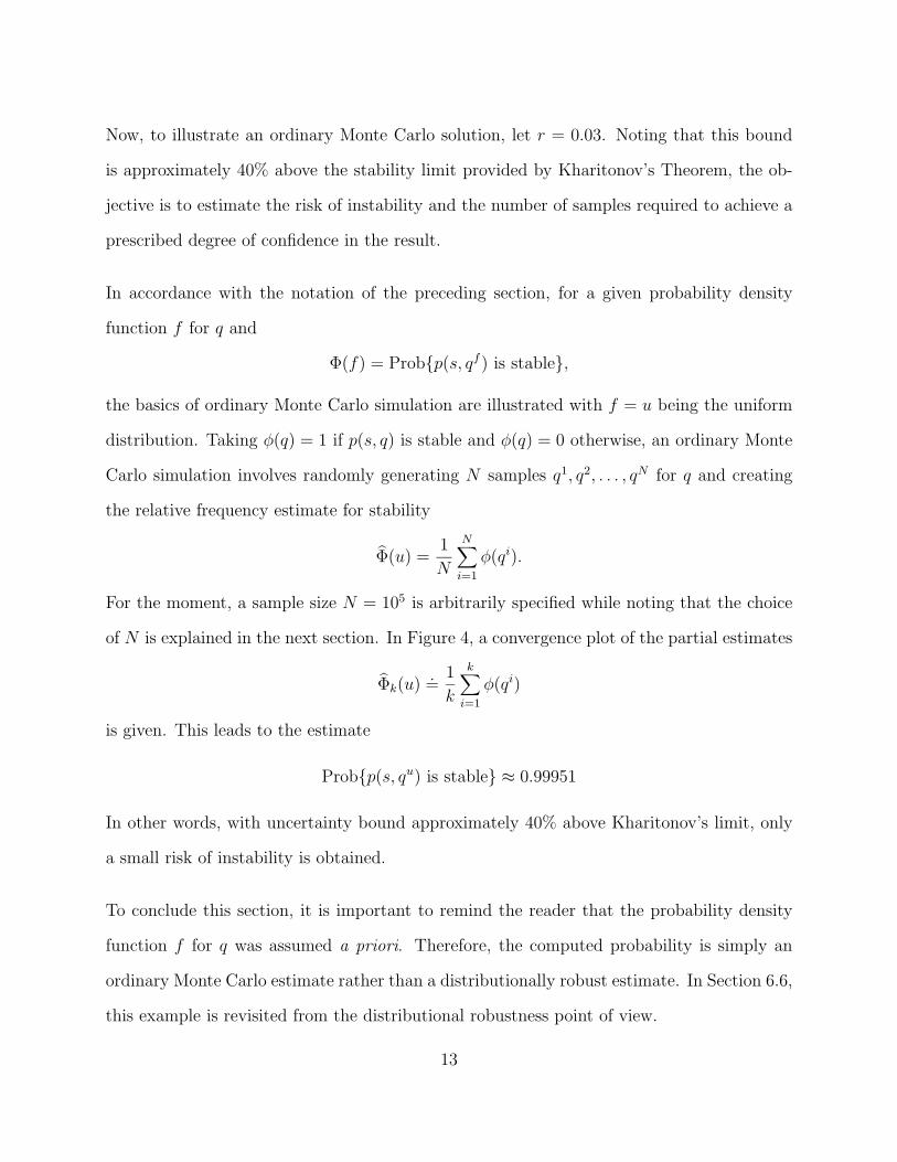
setting, we concentrate on two specific probabilistic measures, taking the distribution f ∈ Fto be a probability density function. The first measure of interest is the probability of

satisfying the performance specifications; i.e., for desired performance level γ > 0, let

Φ(f) = Probφ(qf ) ≤ γ

=∫q∈Q:φ(q)≤γ

f(q)dq.

The second measure is the expected value of φ(qf ). In this case,

Φ(f) = E [φ(qf )] =∫

Qφ(q)f(q)dq.

With the setup above, the distributional robustness problem is to find f ∗ ∈ F minimiz-

ing Φ(f); i.e.,

Φ(f ∗) = minf∈F

Φ(f),

7

or, equivalently,

Φ(f ∗) ≤ Φ(f)

for all f ∈ F .

2.5 Remarks: Upon solving the problem above for f ∗ ∈ F and using this distribution in a

Monte Carlo simulation, we obtain more reliable estimates of probability and expected value

than would be the case using some ad hoc distribution for q. To illustrate, if stability is of

concern, then for any f ∈ F , it follows that

Probstability under qf ≥ Probstability under qf∗.

Hence, a Monte Carlo simulation performed with some ad hoc distribution f ∈ F instead

of f ∗ leads to an unduly optimistic estimate of performance. From a robustician’s point of

view, it is also of interest to determine the extent to which the worst-case performance

φ∗ .= min

q∈Qφ(q)

differs from the expected performance. To this end, the basic inequality

minq∈Q

φ(q) ≤ E [φ(qf∗)]

can be used to understand the icicle metaphor described in Section 2.2.

The desirability of distributional robustness is seen via a simple illustration: Suppose one

is assessing the probability that a performance specification is met and a distributionally

robust probability estimate p = 0.99 is obtained. Then, this probability is guaranteed no

matter which probability density function f ∈ F is realized. Hence, without the knowledge

of the “true” probability distribution, one can nevertheless be confident about the assessment

of performance. This provides a rationale for a new approach to Monte Carlo simulation

for cases when little or no a priori statistical information about the uncertain parameters is

8

available. Namely, in contrast to classical Monte Carlo methods, which require specification

of a probability distribution f for q a priori, we solve a distributional robustness problem

and select a distinguished distribution f ∗ ∈ F . This a posteriori distribution is used in the

random number generation for the associated Monte Carlo simulation. By proceeding in

this manner, one avoids the need to specify some ad hoc distribution when no statistical

information about the uncertainty is available.

3. The Class of Distributions F

In this section, attention is turned to the class of probability distributions F ; to this point

in the paper, this class has not been specified. The paradigm of [2] is now described and

it is argued that the definition of F is physically meaningful for a large class of problems.

In later sections, it is seen that this definition of F leads to a rich theory characterizing

the distinguished distribution f ∗ ∈ F which is used for Monte Carlo simulation. That is, in

order to carry out computer simulations, the computer program generating random numbers

must be “told” what probability distribution f ∈ F to use.

Based on robustness considerations in the systems sciences, an interval bound description of

the uncertainty is the takeoff point for the new paradigm. Motivated in large measure by

manufacturing considerations, the fundamental assumptions in the exposition to follow are

that the uncertain parameters are independent, large deviations in the parameters qi away

from their nominal values is less probable than small deviations and positive and negative

deviations in the qi are equally likely. In other words, no assumptions made about the

probability distribution other than its salient characteristics above. In Section 3.2, after

making these notions precise, the class F emerges. This setup is reminiscent of formulations

such as Huber’s [10] in the field of robust statistics. In contrast to his formulation and

9

−20 −15 −10 −5 0 5 10 15 200

0.01

0.02

0.03

0.04

0.05

0.06

0.07

0.08

0.09

0.1

Figure 3: Admissible Distributions for Capacitor Uncertainty

others, however, no a priori parameterization of the underlying probability density functions

is assumed. This is explained in more detail below.

3.1 Motivating Example: To motivate the definition of F , consider a circuit with an

uncertain capacitor 30 µfd ≤ C ≤ 70 µfd which is nominally manufactured with nominal

value C0 = 50µfd. For this capacitor, the manufacturing process is modelled by assuming

that positive and negative deviations about C0 are equally likely and that large deviations

from C0 are less likely than small deviations. In other words, if |∆C1| < |∆C2|, then the

capacitor with value C = 50 + ∆C1 is more likely to be manufactured than the resistor with

value C = 50 + ∆C2. This situation is illustrated in Figure 3 where the possible probability

density functions for capacitor uncertainty ∆C are depicted with zero mean. These ideas

are now precisely formulated in the more general setting of this paper.

10

3.2 Class of Admissible Distributions F : It is assumed that the uncertainty vector q is

a zero mean random vector with independent components qi. Furthermore, for i = 1, 2, . . . , ,

it is assumed that each component qi is supported in the interval

Qi.= [−ri, ri].

Therefore, the support for the random vector q is the hypercube

Q = Q1 × Q2 × · · · × Q.

Now, a density function fi(xi) is said to be admissible for qi if it is symmetric and non-

increasing with respect to |xi|. More precisely, fi is an admissible probability density function

for qi if

fi(xi) ≥ fi(yi),

for |xi| ≤ |yi| and

fi(xi) = fi(−xi)

for all xi.To make the definition of F complete, the behavior of fi(xi) at xi = 0 needs to be

specified. In this paper, fi(xi) is allowed to be a probability density function which contains

a Dirac delta function at xi = 0. Finally, by writing f ∈ F for the joint density function

f(x).= f(x1, x2, . . . , x) = f1(x1)f2(x2) · · · f(x)

of the random vector qf , the understanding is that each fi is an admissible probability density

function for qi.

3.3 Distributionally Robust Performance: As indicated in Section 2.4, each admissible

density function f ∈ F results in a value Φ(f) for system performance. Now, we define the

distributionally robust cost

Φ∗ .= inf

f∈FΦ(f).

11

Since it has not yet been guaranteed that the infimum above is attained for some f ∗ ∈ F , we

use the “inf” notation for the definition above. This “inf” will later be sharpened to “min”

in the results to follow.

3.4 Summary: The fundamental difference between “ordinary” Monte Carlo theory and

distributionally robust Monte Carlo theory is as follows: In the ordinary Monte Carlo prob-

lem, the probability density function f used in the simulation is specified a priori. In the

distributionally robust Monte Carlo problem, f is determined a posteriori; that is, one solves

a variational problem to obtain f ∗ ∈ F minimizing Φ(f).

3.5 Preview Example: To consolidate the development to date and preview the expo-

sition to follow, an example from the theory of robust stability, for example, see [50], is

provided to demonstrate some of the basic ideas. To this end, we consider the theory of

interval polynomials based on Kharitonov’s Theorem [51] within the probabilistic setting of

this paper. For the uncertain polynomial

p(s, q) = p0(s) +14∑i=1

si−1qi

with interval bounds qi ∈ [−r, r] for i = 1, 2, . . . , 12 and stable nominal

p0(s) = (s + 1)12(s2 + 0.002s + 1),

with lightly damped roots s = −0.001 ± j and good set

Qgood = q ∈ Q : p(s, q) is stable,

we compare a classical Monte Carlo solution of the stability problem with the robust solution.

Whereas ordinary Monte Carlo is used here, in Section 6.6, this same problem is revisited

from the distributional robustness point of view.

First, using Kharitonov’s Theorem [51], robust stability for p(s, q) is guaranteed if

r < 0.021.

12

Now, to illustrate an ordinary Monte Carlo solution, let r = 0.03. Noting that this bound

is approximately 40% above the stability limit provided by Kharitonov’s Theorem, the ob-

jective is to estimate the risk of instability and the number of samples required to achieve a

prescribed degree of confidence in the result.

In accordance with the notation of the preceding section, for a given probability density

function f for q and

Φ(f) = Probp(s, qf ) is stable,

the basics of ordinary Monte Carlo simulation are illustrated with f = u being the uniform

distribution. Taking φ(q) = 1 if p(s, q) is stable and φ(q) = 0 otherwise, an ordinary Monte

Carlo simulation involves randomly generating N samples q1, q2, . . . , qN for q and creating

the relative frequency estimate for stability

Φ(u) =1

N

N∑i=1

φ(qi).

For the moment, a sample size N = 105 is arbitrarily specified while noting that the choice

of N is explained in the next section. In Figure 4, a convergence plot of the partial estimates

Φk(u).=

1

k

k∑i=1

φ(qi)

is given. This leads to the estimate

Probp(s, qu) is stable ≈ 0.99951

In other words, with uncertainty bound approximately 40% above Kharitonov’s limit, only

a small risk of instability is obtained.

To conclude this section, it is important to remind the reader that the probability density

function f for q was assumed a priori. Therefore, the computed probability is simply an

ordinary Monte Carlo estimate rather than a distributionally robust estimate. In Section 6.6,

this example is revisited from the distributional robustness point of view.

13

0 1 2 3 4 5 6 7 8 9 10

x 104

0.993

0.994

0.995

0.996

0.997

0.998

0.999

1

1.001

N

Est

imat

e of

Pro

babi

lity

of S

tabi

lity

Figure 4: Estimated Probability of Stability Versus Sample Size N

3.6 Sample Generation: Although not the focal point of this paper, it is important to

provide an indication of how one generates the random samples and how one chooses the

sample size. Since these problems are important in both the classical and the distributionally

robust Monte Carlo settings, some highlights in the sample generation and sample size

literature are now described.

Currently, many software packages contain routines for generating random samples with

commonly used distributions. For example, the basic distribution of Matlab contains routines

for generating samples with either uniform or Gaussian distributions. However, when dealing

with robustness problems, one is confronted with the necessity of generating samples with

distributions other than the ones mentioned above. For example, when using Monte Carlo

methods for analyzing systems with unstructured uncertainty, one might have uncertainty

that is uniformly distributed on a sphere. For cases like this, one needs more powerful tools

for sample generation; see [5] for a comprehensive treatment.

14

Of special interest to robusticians, is the problem of generating samples uniformly distributed

over a given compact convex set. This problem has been addressed by several authors; we

mention two approaches which have been proposed. The first approach involves the design of

a Markov chain whose stationary distribution is the required one. Examples of this approach

can be found in [5] and [7], where algorithms have been proposed for very general compact

convex sets. For cases when one has a lot of information about the convex set in which we

want the samples to be generated, one can develop more direct sample generation algorithms

which do not rely on the asymptotic behavior of a Markov chain. For example, this is the

case addressed in [8] and [9]. where algorithms are provided for uniform sampling over p

ball described by

qp1 + qp

2 + · · · + qp ≤ 1

and over the “sphere” of matrices

M .= A ∈ Rn×n : σ(A) ≤ 1

where σ(A) denotes the maximum singular value of the matrix A.

3.7 Sample Size: In the literature on sample generation, the following question arises:

For a given uncertainty dimension and a given probability density function f for q, how

many samples N are required to obtain a “reliable” estimate ΦN(f)? Surprisingly, with

reliability defined in terms of probable approximate correctness (PAC) as indicated below,

it can be shown that there are upper bounds for the required number of samples which

are independent of both and f . To illustrate the use of such results, following [42], the

PAC reliability criterion is defined and illustrated using sample size bounds provided in [39]

and [40].

3.8 Reliability Based on Probable Approximate Correctness: In this framework,

the estimate ΦN(f) is viewed as random variable and one seeks to find probability of this

15

quantity being in error by no more than a prescribed tolerance ε > 0. With this setup, an

estimate ΦN(f) is said to have reliability of 0 < δ < 1 if

Prob|ΦN(f) − Φ(f)| > ε ≤ δ.

In other words, the probability of an estimation error exceeding ε is less than or equal to δ.

With the definition above, there are many papers with upper bounds on the number of

samples N = N(ε, δ) which are needed; e.g., see [39] and [40]. To illustrate, a simple upper

bound based on the Law of Large Numbers is

N(ε, δ) =1

4ε2δ.

A second upper bound, obtained using the Bienayme inequality is

N(ε, δ) =

√3

4ε2√

δ.

A third upper bound, obtained using the Chernoff inequality is

N(ε, δ) =ln(2/δ)

2ε2.

None of the bounds above is “best” in the sense of requiring less samples than the others

for all (ε, δ) pairs. Therefore, for a given ε and δ, one can look at all available bounds and

take the smallest of the N(ε, δ) values obtained. To illustrate, using the three bounds above

with ε = 0.01 and δ = 0.06, the Bienayme bound is the tightest and leads to N ≈ 1.77 × 104.

For the tighter specification ε = δ = 0.001 corresponding to a 0.1% error, one obtains

N ≈ 3.8 × 106 using the Chernoff bound.

For the case of the interval polynomial in Section 3.5 above, ε = δ = 0.005 was taken as the

reliability specification and the number of samples dictated is N = 1.2× 105. However, as a

practical matter, it is seen in Figure 4 that with N = 3 × 104, convergence is obtained with

far fewer samples than that prescribed by the theory. This is consistent with the authors’

experience involving Many Monte Carlo case studies of this sort.

16

4. The Truncation Principle

The Truncation Principle of [2] is a fundamental result in the theory of distributional robust-

ness and serves as the takeoff point for the Monte Carlo simulation techniques in the sequel.

This principle indicates that when minimizing the performance functional Φ(f) over f ∈ F ,

one need only consider truncated uniform distributions. In other words, it turns out to be

the case that distributional robustness is achieved by restricting attention to probability

distributions which are constant over some subinterval [−ti, ti] of [−ri, ri]. For example,

even though a truncated normal distribution is admissible, it can be ignored when minimiz-

ing Φ(f) over f ∈ F . This means that the prescription for distributionally robust simulation

involves sampling only a subinterval of the uncertainty rather than the entire interval.

It is interesting that the subinterval sampling scheme above may seem counterintuitive in

certain applications. For example, for Monte Carlo simulation of a system with spring

constant parameter 0.4 ≤ k ≤ 0.6, a distributionally robust simulation may require sampling

restricted to 0.45 ≤ k ≤ 0.55. These ideas are now formalized.

4.1 Truncated Uniform Distributions: A probability density function ut(x) is called a

truncated uniform distribution if each of its components uti(xi) is either distributed uniformly

over a symmetric interval [−ti, ti] ⊆ [−ri, ri] for ti > 0 or zero with probability one for ti = 0;

that is, a Dirac delta function. The interval [−ti, ti] might be different for each uncertainty

component. Using the notation

T.= t = (t1, t2, . . . , t) ∈ R : 0 ≤ ti ≤ ri for i = 1, 2, . . . , ,

for t ∈ T , we take

ut(x).= ut

1(x1)ut2(x2) · · · ut

(x)

17

− r1− t1

r1t1− t2 t2− r2 r2

x1 x2

f x1 1( ) f x2 2( )

Figure 5: Truncated Uniform Distribution

to be the associated truncated uniform distribution. For the special case obtained with ti = ri

for i = 1, 2, . . . , , one obtains the uniform distribution u(x) over Q. It is also observed that

all truncated uniform distributions ut belong to the class F ; i.e., the inclusion

ut : t ∈ T ⊆ F .

holds. An example of a truncated uniform distribution for = 2 is presented in Figure 5.

The Truncation Principle of [2] indicates that, in the search for the minimum of Φ(f), one

need not to consider all possible distributions f ∈ F ; that is attention can be restricted to

the class truncated uniform distributions ut obtained with t ∈ T .

4.2 The Truncation Principle: With the notation above,

inff∈F

Φ(f) = inft∈T

Φ(ut).

4.3 Distributional Robustness: The theorem above provides a prescription for distribu-

tionally robust Monte Carlo simulation for many cases when some optimal truncation t∗ ∈ T

minimizing Φ(ut) can be found. Namely, one simply performs the simulation using uniform

sampling over the interval [−t∗i , t∗i ] in lieu of [−ri, ri].

4.4 Example Illustrating Truncation Principle: The Truncation Principle raises the

possibility that distributionally robust Monte Carlo simulation may lead to results which dif-

fer significantly from what one might obtain using a more traditional Monte Carlo approach.

18

1

L

I

+

-

CC R V1 2 021R

Figure 6: RLC Circuit

That is, in the example below, taken from [30], the Truncation Principle leads to sampling

over a subinterval of the range of qi whereas a classical Monte Carlo analysis typically dic-

tates sampling over the entire range of parameter variation. Subsequently, the two methods

may lead to dramatically different assessments of performance. In this regard, the point of

view in this paper is that traditional Monte Carlo simulation provides an unduly optimistic

estimate of the performance whereas the distributionally robust approach does not.

The RLC circuit of [30] is now studied with random parameters corresponding to independent

uncertainties in the interstage capacitors C1 and C2; see Figure 6. The amplifier has fixed

parameters R1 = 1000, R2 = 100, L = 0.01 and uncertain parameters

0.755 × 10−6 ≤ C1 ≤ 1.695 × 10−6; 0.75 × 10−6 ≤ C2 ≤ 4.55 × 10−6.

For this example, performance is defined in terms of the overshoot to a step input. The

specification is that |V0(t)| not exceed 96.3 volts. This leads to an interest in computing the

probability that this performance specification is satisfied.

To study this circuit using the Truncation Principle, q1 and q2 are identified with deviations

from the center points of the intervals of capacitance. Next, letting V0(q1, q2, t) denote the

dependence of the output voltage on the qi and taking

Q.= (q1, q2) : |q1| ≤ r1 = 0.940 × 10−6; |q2| ≤ r2 = 4.8 × 10−6

19

and

Qgood.= (q1, q2) : |V0(q1, q2, t)| ≤ 96.3 for all t ≥ 0,

we seek to compute the distributionally robust performance

Φ∗ .= min

f∈FProbqf ∈ Qgood.

In accordance with the Truncation Principle, a solution to this problem is obtained with

marginals uti which are truncated uniform distributions described by ti . For the given

uncertainty bounds for the two capacitors variations, a two variable optimization in the

truncation variable t.= (t1, t2) ∈ T was carried out. Using the Matlab rand function to

estimate

pt.= Probqut ∈ Qgood

and generating 100,000 samples for (t1, t2) pairs, the estimate

Φ∗ = Φ(ut∗) = pt∗ ≈ 0.486

was reached with truncations given by t1 = t∗1 ≈ 0.17 × 10−6 and t2 = t∗2 ≈ 0.275 × 10−6.

This result is shown in the contour plot in Figure 7. It is noted that the truncation t∗

maximizing pt is obtained as an interior point within the rectangle of capacitor variation.

In order to compare the result above with a traditional Monte Carlo simulation, we take f = u

to be the uniform distribution and obtain the estimate

Φ(u) = Probqu ∈ Qgood ≈ 0.6912,

which is more than 50% larger than Φ∗.

4.5 Remarks: The successful use of the Truncation Principle to solve the circuit prob-

lem above was facilitated by the fact that the uncertain parameter vector q was only two-

dimensional. For problems with higher dimensional uncertainty, finding an “optimal trunca-

tion” t∗ is generally a nonlinear programming problem. Whereas a gridding method sufficed

20

0 0.5 1 1.5 2 2.5 3 3.5 4 4.5

x 10−7

0

0.2

0.4

0.6

0.8

1

1.2

1.4

1.6

1.8

x 10−6

t1

t2

Figure 7: Contours of Equal Probability in the (t1, t2) Plane

for the circuit illustration above, for a high number of uncertainties, such an approach is

no longer computationally tractable. This motivates an ongoing line of research aimed at

exploiting the structure of the probabilistic robustness problem at hand in order to obtain

an optimal truncation t∗ ∈ T . For example, as seen in Sections 5.1–5.7, for large classes of

circuit configurations, the equations associated the Kirchoff’s laws for circuits make it pos-

sible to characterize the optimal truncation t∗ without recourse to nonlinear programming.

A second case where one can actually determine t∗ occurs when the good set Qgood is convex

and symmetric. As seen in Section 5.9, in this case, the uniform distribution u turns out

to be the optimal truncation; i.e., we set each ti to its maximum value ri. In other words,

in this special case it can be argued that the traditional Monte Carlo approach leads to a

distributionally robust result. Finally, it is also worth mentioning the case when Qgood is

convex but not necessarily symmetric, the concept of symmetrization proves useful to obtain

a bound on the performance function Φ(f) using the uniform distribution; see Section 6.1.

21

5. The Convex and Componentwise Convex Cases

In the absence of an a priori statistical description of the uncertain parameters, it has

been argued that one may obtain unduly optimistic results using traditional Monte Carlo

simulation. In this section, we provide conditions under which the traditional approach

agrees with the distributionally robust approach. In other words, under the conditions

described below, there is indeed a solid rationale for use of the folk theorem which says:

When in doubt, use the uniform distribution. To this end, of the results of [2]–[4] are now

described.

The first result below applies to the case when Φ(f) is the expected value of some componen-

twise convex performance function; i.e., for each i = 1, 2, . . . , , the function φi(qi) obtained

with qk held fix for k = i, is convex in qi. To illustrate, for large classes of robustness

problems with a so-called multilinear uncertainty structure, this componentwise convexity

condition is satisfied; e.g., one can obtain a performance function of the form

φ(q) = 3q1q2q3 + 10q1q2 − 9q1q3 − q2 + 15.

Two examples are provided, which illustrate the application of the Componentwise Convexity

Principle to resistive networks and to H∞ performance. The second result, the Uniformity

Principle in Section 5.9, applies to the case when Φ(f) is the probability of performance

satisfaction and the set Qgood is convex and symmetric (if q ∈ Qgood, then −q ∈ Qgood).

Associated with each of these results, examples are given which illustrate the satisfaction of

the required conditions on Φ(f) and Qgood

5.1 The Componentwise Convexity Principle: If φ(q) is convex with respect to com-

ponent qk, then the minimization of E(φ(qf )) is attained with f ∗ ∈ F having k-th compo-

nent f ∗k = δ, the Dirac delta function. Similarly, if φ(q) is concave with respect to qk then,

the minimization of E(φ(qf )) is attained with f ∗ ∈ F having k-th component f ∗k = u, the

22

uniform distribution.

5.2 Remark: The result above provides conditions under which a minimizing truncation t∗k

in Theorem 4.2 is attained at an extreme t∗k = 0 or t∗k = rk.

5.3 Resistive Networks: For a large class of resistive networks described below, it is seen

that the extreme point solutions obtained above solve the distributional robustness problem

for the expected gain. Such a result is considerably at odds with what one obtains using

Monte Carlo sampling scheme or common sense traditional considerations; i.e, in such a

case, the prescription of the theorem is that some uncertain parameters, those with the

Dirac Delta function distribution, should be held fixed at their nominal values whereas

other uncertain parameters should be sampled uniformly over their range of variation. In

other words, one should resist the temptation to sample those uncertain parameters qk

corresponding to f ∗k = δ in the Componentwise Convexity Principle. To illustrate, if t1 = 0

for q1 and t2 = r2 for q2, then to obtain a distributionally robust performance estimate,

one should ignore the temptation to sample q2 uniformly over its range [−r2, r2]. Instead,

one should generate samples (q1, q2) with q1 fixed at its nominal value and q2 uniformly

distributed over [−r2, r2].

The situation above is more fully described in [34] where the authors consider a planar net-

work N consisting of an input voltage source Vin, an output voltage Vout across a designated

resistor Rout = Rn and uncertain positive resistor n-tuple R.= (R1, R2, . . . , Rn); see Figure 8.

With qi identified with resistor uncertainty ∆Ri representing deviations from the nominal

manufacturing value Ri,0 > 0 and gain

g(q).=

Vout(q)

Vin

,

the Truncation Principle applies to the problem of finding the maximum and minimum values

23

ResistiveNetwork

+nR-inV

-

+

outV

Figure 8: Network Configuration

of the expected gain

E(g(qf )) =∫

Qf(q)g(q)dq.

The definition below, given in [34], leads to the delineation of a class of circuits for which

the optimal truncations for Monte Carlo admit extreme point solution per Section 5.1.

5.4 Essential Resistors: For the class of resistive networks under consideration, phys-

ical interpretations of componentwise convexity and concavity are available. Namely, a

resistor Rk is said to be essential if the following condition holds: There does not exist ad-

missible values of the n − 1 remaining resistors Ri, i = k making the gain g independent

of Rk. If Rk is essential, it can readily be shown that, with qk = ∆Rk as identified above,

the gain is either componentwise convex or concave with respect to qk. To make the con-

vexity/concavity assignment more precise, it is noted that essentiality guarantees that the

partial derivative ∂g/∂qk has one sign over Q. Letting

sk.= sign

(∂g

∂qk

)

denote this invariant sign, exploitation of the Componentwise Convexity Principle leads to

the result of [34] given below.

5.5 Theorem: Assume that all resistors in N are essential. For the case of maximiz-

ing E(g(qf )), define probability density function f ∗ with marginals f ∗i as follows: Set f ∗

i = u

24

if si = −1 and f ∗i = δ if si = 1. Then,

E(g(qf∗)) = max

f∈FE(g(qf)).

For the case of minimizing E(g(qf)), define probability density function f ∗ with marginals f ∗i

as follows: Set f ∗i = δ if si = −1 and f ∗

i = u if si = 1. Then,

E(g(qf∗)) = min

f∈FE(g(qf)).

5.6 Example: To illustrate the use of the theorem above, consider the ladder network

studied in [34] and shown in Figure 9. Applying the theorem above, it can be shown that all

resistors are essential with maximum expected gain being attained by using ti = 0 for the

inter-stage resistors R3k and ti = ri for the remaining resistors. To illustrate how this result is

applied, for a three stage network with nominal values R1,0 = R4,0 = R5,0 = R7,0 = R8,0 = 1,

R2,0 = 2, R3,0 = 3, R6,0 = 5 and R9,0 = 7, and uncertainty bounds ri = 0.8Ri,0 for the inter-

stage resistors and ri = 0.1Ri,0 for the remaining resistors, the results above indicate that

a distributionally robust Monte Carlo simulation should be performed as follows: Hold the

interstage resistors R3, R6 and R9 fixed corresponding to the Dirac Delta function; i.e., do not

sample these parameters despite the fact that sampling ranges are given. For the remaining

resistors, sample uniformly over prescribed ranges [Ri,0− ri, Ri,0 + ri]. This sampling scheme

leads to the estimate

E(g(qf∗)) ≈ 0.1864

with n = 100, 000 samples. In contrast, a more traditional Monte Carlo simulation using the

uniform distribution for all resistors leads to the estimate

E(g(qu)) ≈ 0.1554.

was obtained. In other words, the classical analysis leads to a result which we view as over

optimistic by about 20%.

25

...

...

+

-

VoutVin

R1

R3

R2

R4

R6

R5

Rn-2

Rn

Rn-1

Figure 9: Ladder Network

5.7 Multilinearly Parameterized H∞ Norm: To illustrate a second application of the

Componentwise Convexity Principle, we consider the problem formulation of [36]. Namely,

the starting point is a transfer function matrix H(s, q) which depends multilinearly on the

uncertain vector q. Furthermore, it is assumed that H(s, q) is decomposable as a multilinear

combination fixed stable transfer functions with the uncertain parameters qi being the matrix

multipliers. For example, if H0(s), H1(s), H2(s) and H12(s) are proper stable n×m transfer

function matrices, then

H(s, q) = H0(s) + q1H1(s) + q2H2(s) + q1q2H12(s)

is such a multilinear combination. Another example is obtained from a feedback system

which is set up in the so-called M −∆ configuration with M(s) being a square × proper

stable transfer function matrix and ∆(q) = diagq1, q2, . . . , q. Now,

H(s, q).= det(I + M(s)∆(q))

satisfies the multilinearity requirement of this section.

Using the fact that the norm function is convex and each qi enters affine linearly into H(s, q)

with the remaining parameters fixed, it can readily be shown that that with performance

measure

φ(f) = ||H(s, qf ))||∞,

26

the uncertain parameter vector q enters in a componentwise convex manner. Hence,

maxf∈F

E(||H(s, qf )||∞

)= E (||H(s, qu)||∞) .

In fact, it can also be shown (see [36]) that the same result hold for all moments of ||H(s, q)||∞as well.

5.8 Convex Symmetric Sets: Attention now is turned to the case where Φ(f) is the

probability of performance satisfaction. As seen below, if the set of parameters that satisfy

the performance specifications is convex and symmetric then the the uniform distribution

is the one that should be used in the Distributional Robustness setting. We now formally

present the result of [2] which initiated the distributional robustness line of research.

5.9 The Uniformity Principle: If Qgood is convex and symmetric, then it follows that

minf∈F

Probqf ∈ Qgood = Probqu ∈ Qgood.

Equivalently, the minimizing truncation t∗ in Theorem 4.2 has components t∗i = ri corre-

sponding to the uniform distribution.

5.10 Example (Interval Polynomial): The interval polynomial, analyzed in Section 3.5

from a traditional Monte Carlo point of view is now studied using the Uniformity Principle

It is shown that a distributionally robust under-estimate of the probability of stability can

be obtained using the Uniformity Principle. Indeed, recalling p(s, q) = p0(s) +∑12

i=1 si−1qi

with interval bounds qi ∈ [−r, r] for i = 1, 2, . . . , 12, uncertainty radius r = 0.03 and stable

nominal p0(s) = (s + 1)12(s2 + 0.002s + 1), in lieu of defining Qgood in terms of stability, we

generate this set based on frequency domain considerations. Namely, with target set P(ω)

given in Figure 10, for robust stability, classical robustness theory (for example, see [50]) can

be used to show that with a fixed q ∈ Q, stability of p(s, q) is assured if

p(jω, q) ∈ P(ω)

27

−3 −2 −1 0 1 2 3 4−0.3

−0.2

−0.1

0

0.1

0.2

0.3

0.4

0.5

Figure 10: The Target Set P(ω) for 0.98 ≤ ω ≤ 1.02.

for the critical range of frequencies 0.98 ≤ ω ≤ 1.02.

Now, to obtain the desired distributionally robust Monte Carlo estimate, we take

Qgood.= q ∈ Q : p(jω, q) ∈ P(ω) for 0 ≤ ω < ∞

and note that p0(jω) is the center of the frequency dependent rectangles in Figure 10. Hence,

Qgood is convex and symmetric and the Uniformity Principle applies; that is

pΩ.= min

f∈FProbqf ∈ Qgood = Probqu ∈ Qgood.

Now, an estimate pΩ of pΩ is obtained using a uniform sampling distribution over Q. For

this example, using N = 106 samples, it turns out that

pΩ ≈ 0.9969.

In conclusion, the inequality

pΩ ≤ minf∈F

Probp(s, qf ) is stable,

28

guarantees a distributionally robust probability estimate of stability of at least 0.9969.

5.11 Example (Robust Least Squares): Consider an over-determined set of linear equa-

tions

Ax = b; x ∈ Rn; b ∈ Rm; m ≤ n,

with matrix A ∈ Rm×n having rank m. Given data A = A0 and b = b0, the classical least

squares problem is to as find x = xLS which minimizes the residual cost function

JLS(x).= ‖A0x − b0‖.

It is well known that the solution for this problem is

xLS = (AT0 A0)

−1AT0 b0.

Now, in the presence of data uncertainty, a distributional robustness problem arises: Indeed,

with both A and b having uncertain parameters qi entering affine linearly, we write

A(q).= A0 +

∑i=1

qiAi

and

b(q).= b0 +

∑i=1

qibi

where the n × m matrices and the m × 1 vectors bi above are fixed.

Now, to study this problem using the results in this paper, the uncertain parameter vector q

is assumed to have probability distribution f ∈ F and γ > 0 is taken to be an acceptable

residual cost level. Now, with

Φ(f).= Prob‖A(qf )xLS − b(qf )‖ ≤ γ

and nominal solution xLS satisfying A0xLS = b0, the associated good set

Qgood.= q ∈ Q : ‖A(q)xLS − b(q)‖ ≤ γ

29

is readily shown to be both convex and symmetric. Hence, the Uniformity Principle applies

and it is concluded that

minf∈F

Φ(f) = Φ(u).

5.12 Numerical Example: We now present an example which illustrates application of

the least squares result above. Indeed, with

A(q) =

−1 + q1 −2 + q2 −4 + q3

−5 + q4 5 + q5 −9 + q6

−3 + q7 −3 + q8 −7 + q9

−1 + q10 −2 + q11 −4 + q12

−1 + q13 4 + q14 −1 + q15

and

b(q) = b0 = [−7 − 28 − 14 − 7 − 7]T ,

we first compute the classical least squares solution

xLS = [1 − 1 2]T

corresponding to q = 0. Now, with uncertainty dimension = 15, we assume that the dis-

tribution of the uncertain vector q belongs to the class F and we analyze the performance

of xLS for different radii for the uncertainty. More precisely, we assume that |qi| ≤ r and

study the effects of varying the radius r with xLS held fixed. First, it is noted that clas-

sical robustness theory indicates that the maximum allowed radius is rmax ≈ 0.0112 with

performance specification

‖A(q)xLS − b(q)‖ ≤ 0.1

is satisfied by all allowed values of q if and only if r < rmax ≈ 0.0112. Now, we take the

distributionally robust point of view and seek to compute

Φ∗ = minf∈F

Prob‖A(qf )xLS − b(qf )‖ ≤ γ

30

0 0.005 0.01 0.015 0.02 0.025 0.03 0.035 0.04 0.045 0.050.1

0.2

0.3

0.4

0.5

0.6

0.7

0.8

0.9

1

radius r

Dis

trib

utio

nally

Rob

ust E

stim

ate

rmax

Figure 11: Distributionally Robust Probability of Performance Satisfaction

as a function of the uncertainty radius r. The results obtained are depicted in Figure 11.

To illustrate how conservative a classical robustness measure can be, we take radius of

uncertainty of r = 0.018, which is approximately 60% larger then the rmax. For this radius,

the distributionally robust risk of performance violation is only ε ≈ 0.0001.

For the case of expected performance, it is also interesting to note that least squares analysis

can be carried out for so-called multilinear uncertainty structures. More specifically, con-

sidering the setup above with the entries of A(q) and b(q) depending multilinearly on q, it

follows from the Componentwise Convexity Theorem (see [4] for details) that

maxf∈F

E(‖A(qf )xLS − b(qf )‖) = E(‖A(qu)xLS − b(qu)‖).

31

6. Non-Symmetric and Non-Convex Cases

When Qgood in not convex or symmetric, we seek an optimal truncation t∗ ∈ T , as prescribed

in Theorem 4.2. Since finding t∗ may be computationally complex, it is of interest to circum-

vent this problem. To this end, as illustrated by the polynomial example in Section 5.10, it

is often possible to obtain a lower bound on the probability of performance satisfaction. In

Section 6.1 below, results are given when the convexity property is satisfied but the symme-

try property is violated. In Section 6.3, a method is described which is applicable to cases

for which there exists a deterministic algorithm for testing the satisfaction of performance

specifications on “rectangles” of uncertainty.

6.1 Symmetrization: To motivate the so-called symmetrization approach, consider the

problem of Lyapunov stability with a n×n state space matrix A(q) having entries depending

affinely on the uncertainty vector q and fixed n × n positive-definite Lyapunov matrix P .

Now, consistent with standard Lyapunov theory, for example, see [52], we take

Qgood.= q ∈ Q : AT (q)P + PA(q) < 0.

To motivate the construction below, it is noted that the set Qgood above is readily verified

to be convex but is not necessarily symmetric.

For cases such as the one above, it proves useful to consider the symmetrization of Qgood

given by

Qgood,s.= q : q ∈ Qgood and − q ∈ Qgood.

Now, since Qgood,s is both convex and symmetric, the Uniformity Principle guarantees

minf∈F

Probqf ∈ Qgood,s = Probqu ∈ Qgood,s.

Furthermore, since the containment

Qgood,s ⊆ Qgood

32

holds, the performance estimate obtained using Qgood,s is a lower bound for the true per-

formance. Now, combining these considerations with the applicability of the Uniformity

Principle for Qgood,s, we obtain

Probqu ∈ Qgood,s = minf∈F

Probqf ∈ Qgood,s ≤ inff∈F

Probqf ∈ Qgood.

In practice, it often turns out that this bound is quite useful and the truncation problem is

avoided.

Given that a lower bound on performance is being computed above, the issue of the conser-

vatism of the estimate arises. In this regard, it can be easily seen, using standard reasoning

on probability of sets, that for any f ∈ F ,

Probqf ∈ Qgood ≥ Probqf ∈ Qgood,s ≥ 2 Probqf ∈ Qgood − 1.

In other words, for high performance problems, the bound obtained using symmetrization

becomes tight.

6.2 Example: Figure 12 depicts a mechanical system consisting of four blocks with un-

certain dampers and springs. With eight uncertain parameters with ranges 0.8 ≤ bi ≤ 2.2

and 0.8 ≤ ki ≤ 2.2 for i = 1, . . . , 4 and all unit masses mi = 1, the performance objective

is to keep the gain of the system below a level g for all frequencies. In other words, one

wants to keep the transfer function magnitude |H(jω)| from F to y below g at all frequen-

cies ω ≥ 0. Identifying q1, q2, q3 and q4 with deviations from the center points of the intervals

of spring constants and q5, q6, q7 and q8 with deviations from the center points of the intervals

of damper constants, the theory of Linear Matrix Inequalities, for example, see [52], provides

a sufficient condition for this specification to be satisfied. Namely, with

33

k1

b

k2

2b

k3

3b

k4

4

m =12

m =11 m =13

m =14

b1

y

F

Figure 12: Mechanical System

A0.= A(0) =

0 1 0 0 0 0 0 0−1.5 −1.5 1.5 1.5 0 0 0 0

0 0 0 1 0 0 0 01.5 1.5 −3 −3 1.5 1.5 0 0

0 0 0 0 0 1 0 00 0 1.5 1.5 −3 −3 1.5 1.50 0 0 0 0 0 0 10 0 0 0 1.5 1.5 −3 −3

,

B0 = B(0) =[0 1 0 0 0 0 0 0

]T, C0 = C(0) =

[1 0 0 0 0 0 0 0

],

M0.=

A0S + SAT0 SCT

0 B0

C0S −gI 0BT

0 0 −gI

,

∆A(q) having the appropriate uncertainties corresponding to the non-zero entries of A0

and ∆B(q) = ∆CT (q) = 0, performance is guaranteed if

M0 + ∆M(q) < 0

where

∆M(q).=

∆A(q)S + S∆AT (q) S∆CT (q) ∆B(q)∆C(q)S 0 0∆BT (q) 0 0

.

Taking

Qgood.= q : M0 + ∆M(q) < 0

34

and noting that this set is convex but not symmetric, symmetrization was used to assess the

probability of performance satisfaction. A performance level of g = 6.2076 was considered

and 20,000 samples were used to estimate performance. The value obtained via a Monte

Carlo simulation was

minf∈F

Probqf ∈ Qgood,s = Probqu ∈ Qgood,s ≈ 0.99.

Hence, in this case, we obtain an estimate of probability of performance satisfaction which

satisfies

0.99 ≤ inff∈F

Probqf ∈ Qgood ≤ 0.995.

6.3 Unirectangularity: In this section, we describe the method in [29] which applies to

many cases when the set Qgood is non-convex. Central to this method is the concept of a

unirectangular set which is described below.

As a first step, we define the concept of rectangular projection. That is, given a point q ∈ R,

its rectangular projection R(q) is taken to be the box whose extremes are the point q and

the origin. Namely,

R(q).= (α1q1, α2q2, . . . , αq) : αi ∈ [0, 1] for i = 1, 2, . . . , .

Now, a set Qgood is said to be unirectangular if the rectangular projection of any point q

belonging to Qgood is contained in Qgood; i.e., if q ∈ Qgood then R(q) ⊆ Qgood. An example of

a unirectangular set is shown in Figure 14. The result below, established in [29], motivates

some of the analysis to follow.

6.4 Unirectangularity Principle: If Qgood is unirectangular then,

minf∈F

Probqf ∈ Qgood = Probqu ∈ Qgood.

35

( , , )00 3q

( , , )q q q1 2 3

( , , )q q1 20

q1

q2

q3

Figure 13: Rectangular Projection Set

1q

2q

Figure 14: A Unirectangular Set

36

6.5 Continuation of Unirectangularity: The fact that a Uniformity Principle is also

valid for unirectangular sets is the basis for the method described in [29]. This method is

applicable to all problems for which there exists a deterministic algorithm A which can test

if a given rectangle is contained in Qgood. More specifically, to obtain a lower bound on the

probability of performance satisfaction, for a given uncertainty box Q, let

A(Q).=

1 if q ∈ Qgood for all q ∈ Q;0 otherwise.

For example, if A corresponds to an algorithm for testing some inequality guaranteeing

satisfaction of the desired performance specifications, then A(Q) = 1 indicates that this

inequality is satisfied for all q ∈ Q. Another possibility is that the algorithm A corresponds to

the implementation of some robustness result such as Kharitonov’s Theorem or a structured

singular value criterion.

Next, we describe the method for estimating the probability of performance. In accordance

with [29], if one draws N samples q1, q2, . . . , qN uniformly distributed over Q, it can be shown

that

inff∈F

Probqf ∈ Qgood ≥∑N

i=1 A(R(qk))

N.= p.

Hence, the estimate p above is a lower bound on the probability of performance satisfaction.

6.6 Example (Interval Polynomial): For the second time, the interval polynomial of

Section 3.5 is revisited with the same uncertainty bound ri = 0.03 for i = 1, 2, . . . , 12. In

this case, the algorithm A corresponds to the application of Kharitonov’s Theorem. That

is, A[R(q)] = 1 if the four Kharitonov polynomials associated with R(q) are stable and zero

otherwise. The algorithm above was applied with N = 100, 000 resulting in the estimate

p ≈ 0.99936.

37

7. Spherical Setting: A Brief Introduction

Thus far, this paper has concentrated on cases with the so-called structured uncertainty

entering the model. In this section, we consider cases where the uncertainty is unstruc-

tured. In this regard, the method for analysis of unstructured uncertainty of [31] is briefly

introduced. In this new setting, the first point to note is that the description of F given in

Section 3.2 is unsuitable. That is, for the case of unstructured uncertainty, it is unreasonable

to assume that the uncertain parameters vary independently. This observation motivates a

new definition for the set of probability distributions F so as to accommodate parameter

dependency.

7.1 New Definition of the Class F : Using the Euclidean norm for q and taking

Q.= q : ‖q‖ ≤ r,

a probability density function f is said to belong to the class F if there exists a nondecreasing

function g(·) with scalar argument such that

f(x) = g(‖x‖)

for all x. Intuitively, this says that larger uncertainty values are less likely than smaller

values and that all uncertainty “directions” are equally probable.

7.2 Truncations: Analogous to the development in Sections 1–6, in this spherical setting,

a class of radially truncated uniform distributions is defined. Indeed, letting 0 ≤ t ≤ r

denote a truncation radius, the truncated uniform distribution ut is the uniform distribution

over the truncated sphere

Qt.= q : ‖q‖ ≤ t.

For example, if Q is the unit sphere, then the uniform distribution over the sphere of ra-

dius t = 1/3 would be a radial truncation.

38

In this radial distribution framework, perhaps a most important observation is that there is

only one truncation parameter, no matter what the dimension of q. Therefore, the problem

of finding a optimal truncation t∗ ∈ T is greatly simplified. That is, one need only conduct

a single variable line search in the variable t.

7.3 Truncation Principle: Analogous to the case of independent uncertainty, it is shown

in [31] that the Truncation Principle

inff∈F

Φ(f) = inft∈T

Φ(ut)

also holds in the spherical uncertainty case. As seen in the example below, this result readily

lends itself to numerical computation.

7.4 Example: To illustrate a typical problem which is addressed in the spherical setting,

consider the n-dimensional state space system

x = A(q)x

having uncertain matrix A(q) which is partially structured and given by

A(q).= A0 + B0∆(q)C0

where A0 is a fixed nominal state matrix, B0 is a fixed n × m matrix, C0 is a fixed r × n

matrix and ∆(q) is an m × r random matrix representing the uncertainty. Now, with Q

being a sphere representing unstructured variations and

Qgood.= q ∈ Q : A0 + B0∆(q)C0 is stable,

we consider the problem of finding t∗ ∈ T leading to

mint∈T

Probqut ∈ Qgood = Probqut∗ ∈ Qgood.

39

Now, with the specific problem data

A0 =

0 1 0 0 00 0 1 0 00 0 0 1 00 0 0 0 1

−6812 −3090.6 −913.6 −235.10 −28.1

;

B0 =[0 0 0 0 −1

]T;

C0 =

[520 226 56 11 115.6 6.78 1.68 0.33 0.03

],

it follows that

∆ = [q1 q2]

is a 2-dimensional row vector and Property P is deemed to be satisfied if and only if the

uncertain matrix A = A0 + B0∆C0 is stable. Now, using the Truncation Principle in this

spherical setting with uncertainty radius r = 13.188 and N = 300, 000 samples, the function

Φ(t) = Probut ∈ Qgood

is studied and found to have minimizer t∗ ≈ 11.78; this which corresponds to a probability of

stability Φ(t∗) ≈ 0.8149. In contrast, with uniform distribution, one obtains Φ(r) ≈ 0.8193.

That is, common sense use of the uniform distribution in lieu of ut∗ leads to a probability

estimate which is slightly more optimistic than the distributionally robust result.

7.5 Uniformity Principle: For the case of spherical uncertainty, it is shown in [31] that

a Uniformity Principle holds under weaker hypothesis than in the independent parameter

case. That is, instead of requiring Qgood to be convex and symmetric, we only require Qgood

to be star-shaped; i.e., if q ∈ Qgood then λq ∈ Qgood for all λ ∈ [0, 1].

40

An example illustrating satisfaction of the star-shaped requirement is obtained from the the-

ory of quadratic stability. Indeed, suppose that A0 is an n×n stable matrix and P = P T > 0

is an n × n candidate Lyapunov matrix satisfying

AT0 P + PA0 < 0.

Now, suppose A0 is replaced by A = A0+∆A(q) and we want to determine how large ||∆A(q)||can be while preserving the stability inequality above. Then, if ∆A(q) is a linear function

of q and

Qgood.= q ∈ Q : AT P + PA < 0,

it is easy to verify that the resulting set Qgood is star-shaped. Hence, in view of the Uniformity

Principle, a uniform sampling scheme can be used in a distributionally robust Monte Carlo

simulation.

8. Conclusion

Distributionally robust Monte Carlo simulation is a research area which is still in its infancy.

As seen in this paper, many of the problems in the area reduce to finding a so-called optimal

truncation vector t∗ ∈ T which defines the required interval for uniform sampling. It was also

seen that there are many special cases for which this truncation-finding problem is readily

solved. For example, when Qgood is convex and symmetric, the Uniformity Principle was seen

to apply; i.e., one simply takes all t∗i = ri corresponding to a uniform distribution. A second

special case was seen to involve classes of circuits for which distributional robustness was

obtained with an extreme distribution, uniform or impulsive. Finally, a number of special

cases were described for which one obtains a distributionally robust lower bound for the

probability of performance satisfaction.

41

By way of future research, there are many open problems involving some aspect of truncation-

finding. Most notably, when the performance specification function φ(q) comes from a spe-

cific physical generating mechanism, analogous to the case of resistive networks in Section 5.3,

it is of interest to investigate the extent to which exploitation of the structure of φ may lead

to a solution of the truncation problem. In this regard, there are many control theoretic

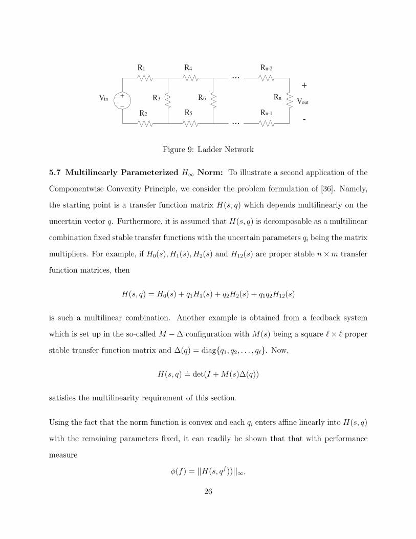
problems of interest. To illustrate, if H(s, q) is a transfer function obtained from a sig-

nal flow graph with uncertain branch gains qi, the manner in which these gains enter H

might be exploited to find the desired truncations t∗i . This is simply one of many examples

of problems with a system theoretic flavor which would be worthy of investigation in the

distributional robustness framework. Finally, it is felt that further research involving the

spherical setting of Section 7 would be worthwhile. For problems lending themselves to this

setting, truncation-finding is not a serious problem because only one truncation parameter

is involved.

A second important line of future research involves what might appropriately be termed

distributionally robust design. To this end, it should be noted the results described in this

paper were entirely of an analysis nature; i.e., there were no design variables entering the

performance specification φ(q). It would be of interest to extend the results reported here

classes of problems for which a design vector x enters φ. For example, one considers a

performance specification φ(x, q) and the goal is to select x so as to provide the best possible

level of performance which is distributionally robust with respect to f ∈ F . Some initial

results in this area are given in [3] and [44].

42

References[1] Rubinstein, R. Y. (1981). Simulation and the Monte Carlo Methods, Wiley, New York.

[2] Barmish, B. R. and C. M. Lagoa (1997). “The Uniform Distribution: A Rigorous Justifi-

cation for its Use in Robustness Analysis,” Mathematics of Control Signals and Systems,

vol. 10, pp. 203-222.

[3] Lagoa, C. M. (1998). Contributions to the Theory of Probabilistic Robustness, Ph.D.

Dissertation, ECE Department, University of Wisconsin, Madison.

[4] Barmish, B. R. and P. Shcherbakov (1999). “Distributionally Robust Least Squares,”

Proceedings of the International Symposium on Adaptive Systems, St. Petersburg, Rus-

sia.

[5] Devroye, L. (1986). Non-Uniform Random Variable Generation, Springer-Verlag, New

York.

[6] Chernoff, H. (1952). A Measure of Asymptotic Efficiency for Test of Hypothesis Based

on the Sum of Observations, Annals of Mathematical Statistics, vol. 23, pp. 493–507.

[7] Fok, D. S. K. and D. Crevier (1989). Volume Estimation by Monte Carlo Methods,

Journal of Statistical Computation and Simulation, vol. 31, pp. 223–235.

[8] Calafiore, G., F. Dabbene and R. Tempo (1998). “Uniform Sample Generation in lp Balls

for Probabilistic Robustness Analysis,” Proceedings of the IEEE Conference on Decision

and Control, Tampa.

[9] Calafiore, G., F. Dabbene and R. Tempo (2000). “Randomized Algorithms for Proba-

bilistic Robustness With Real and Complex Structured Uncertainty,” IEEE Transactions

on Automatic Control, AC–45, pp. 2218–2235.

[10] Huber, P. J. (1981). Robust Statistics, John Wiley & Sons, New York.

43

[11] Barmish, B. R. and B. T. Polyak (1996). “A New Approach to Open Robustness

Problems Based on Probabilistic Prediction Formulae,” Proceedings of the IFAC World

Congress, San Francisco.

[12] Chen X. and K. Zhou (1997). “A Probabilistic Approach to Robust Control,” Proceed-

ings of the IEEE Conference on Decision and Control, San Diego.

[13] Chen, X. and K. Zhou (1998). “Constrained Optimal Synthesis and Robustness Anal-

ysis by Randomized Algorithms,” Proceedings of the American Control Conference,

Philadelphia.

[14] Gazi, E., W. D. Seider and L. H. Ungar (1997). “A Non-parametric Monte Carlo Tech-

nique for Controller Verification,” Automatica, vol. 33, pp. 901–906.

[15] Marrison, C. and R. Stengel (1994). “The Use of Random Search and Genetic Al-

gorithms to Optimize Stochastic Robustness Functions,” Proceedings of the American

Control Conference, Baltimore.

[16] Petersen, I. R. , S. O. R. Moheimani and H. R. Pota (1999). “Minimax LQG Optimal

Control of Acoustic Noise in a Duct,” Proceedings of the World Congress of IFAC,

Beijing, China.

[17] Ray, L. R. and R. F. Stengel (1993). “A Monte Carlo Approach to the Analysis of

Control System Robustness,” Automatica, vol. 29, pp. 229–236.

[18] Stengel, R. F. and L. R. Ray (1991). “Stochastic Robustness of Linear Time-Invariant

Control Systems,” IEEE Transactions on Automatic Control, AC–36, pp. 82–87.

[19] Stengel, R. F., L. R. Ray and C. I. Marrison (1995). “Probabilistic Evaluation of Control

Systems Robustness,” International Journal of Systems Science, vol. 26, pp. 1363–1382.

44

[20] Yoon, A., P. Khargonekar and K. Hebbale (1997). “Design of Computational Experi-

ments for Open-Loop Control and Robustness Analysis of Clutch–to–Clutch Shifts in Au-

tomatic Transmissions,” Proceedings of the American Control Conference, Albuquerque.

[21] Zhu, X., Y. Huang and J. Doyle (1996). “Soft vs. Hard Bounds in Probabilistic Robust-

ness Analysis,” Proceedings of the IEEE Conference on Decision and Control, Kobe,

Japan.

[22] Goodwin, G. C., L. Wang and D. Miller (1999). “Bias-Variance Trade-Off Issues in

Robust Controller Design Using Statistical Confidence Bounds,” Proceedings of the IFAC

World Congress, Beijing.

[23] Zhu, X. (1999) “Probabilistic µ Upper Bound Using Linear Cuts,” Proceedings of the

IFAC World Congress, Beijing.

[24] Calafiore, G., F. Dabbene, R. Tempo. (1999). “The Probabilistic Real Stability Radius,”

Proceedings of the IFAC World Congress, Beijing.

[25] Hara, S. and T. Miyazato. (2000) “A Probabilistic Approach To Robust Control Design,”

Proceedings of the IEEE Conference on Decision and Control, Sydney.

[26] Barmish, B. R., C. M. Lagoa and P. S. Shcherbakov (1996). “Probabilistic Enhancement

of Robustness Margins Provided by Linear Matrix Inequalities,” Proceedings of the

Allerton Conference on Communication, Control and Computing, Monticello.

[27] Barmish, B. R., C. M. Lagoa and R. Tempo (1997). “Radially Truncated Uniform Dis-

tribution for Probabilistic Robustness of Control Systems,” Proceedings of the American

Control Conference, Albuquerque.

[28] Barmish, B. R. and P. S. Shcherbakov (1999). “Distributionally Robust Least Squares,”

Proceedings of SPAS’99, St. Petersburg, Russia.

45

[29] Lagoa, C. M., P. S. Shcherbakov and B. R. Barmish (1998). “Probabilistic Enhancement

of Classical Robustness Margins: The Unirectangularity Concept,” Systems and Control

Letters, vol. 35, pp. 31–43.

[30] Zhang, J., C. M. Lagoa and B. R. Barmish (1998). “Probabilistic Robustness: An

RLC Realization of the Truncation Phenomenon,” Proceedings of the American Control

Conference, Philadelphia.

[31] Barmish, B. R., C. M. Lagoa and R. Tempo (1997). “Radially Truncated Uniform Dis-

tribution for Probabilistic Robustness of Control Systems,” Proceedings of the American

Control Conference, Albuquerque.

[32] Muhler, M. L. and B. R. Barmish, (1999). “A Uniformity Principle for Probabilis-

tic Robustness of the Discrete-Time Linear Quadratic Regulator,” Proceedings of the

American Control Conference, San Diego,.

[33] Shcherbakov, P. S., C.M. Lagoa and B. R. Barmish (1999). “Characterization of

Worst-Case Uncertainty Geometry in the Theory of Probabilistic Robustness,” Pro-

ceedings of the IFAC World Congress, Beijing.

[34] Barmish, B. R. and H. Kettani (2000). “Monte Carlo Analysis of Resistive Networks

Without Apriori Probability Distributions,” Proceedings of the International Symposium

on Circuits and Systems, Geneva, Switzerland.

[35] Kettani, H. and B. R. Barmish (2000). “A New Approach to Monte Carlo Analysis Illus-

trated for Resistive Networks,” Proceedings of the Conference on Information Sciences

and Systems,, Princeton University, Princeton.

[36] Barmish, B. R. (2000) “A Probabilistic Robustness Result For a Multilinearly Param-

eterized H∞ Norm,” Proceedings of the American Control Conference, Chicago.

46

[37] Bai, E.-W., R. Tempo and M. Fu (1997). Worst Case Properties of the Uniform Distribu-

tion and Randomized Algorithms for Robustness Analysis, Proceedings of the American

Control Conference, Albuquerque, New Mexico.

[38] Djavdan, P., H. J. A. F. Tulleken, M. H. Voetter, H. B. Verbruggen and G. J. Ols-

der (1989). “Probabilistic Robust Controller Design,” Proceedings of the IEEE Confer-

ence on Decision and Control, Tampa.

[39] Khargonekar, P. and A. Tikku (1996). “Randomized Algorithms for Robust Constrol

Analysis and Synthesis Have Polynomial Complexity,” Proceedings of the IEEE Confer-

ence on Decision and Control, Kobe, Japan.

[40] Tempo, R., E. W. Bai and F. Dabbene (1996). “Probabilistic Robustness Analysis:

Explicit Bounds for the Minimum Number of Samples,” Proceedings of the IEEE Con-

ference on Decision and Control, Kobe, Japan.

[41] Tempo, R., E. W. Bai and F. Dabbene (1997). “Probabilistic Robustness Analysis:

Explicit Bounds for the Minimum Number of Samples,” Systems and Control Letters,

vol. 30, pp. 237–242.

[42] Vidyasagar, M. (1997). A Theory of Learning and Generalization, Springer Verlag, Lon-

don, England.

[43] Vidyasagar, M. (1997). “Statistical Learning Theory: An Introduction and Applications

to Randomized Algorithms,” Proceedings of the European Control Conference, Brussels,

Belgium.

[44] Barmish, B. R. and C. M. Lagoa (1999). “On the Convexity of the Probabilistic Design

Problem for Quadratic Stabilizability,” Proceedings of the American Control Conference,

San Diego.

47

[45] Director, S. W. and G. D. Hachtel (1977). “The Simplicial Approximation Approach

to Design Centering,” IEEE Transactions on Circuits and Systems, vol. CAS-24,

pp. 363-372.

[46] Director, S. W. and L. M. Vidigal (1981), “Statistical Circuit Design: A Somewhat

Biased Survey,” Proceedings of the European Conference on Circuit Theory Design, The

Hague, The Netherlands.

[47] Pinel, J. F. and K. Singhal (1977). “Efficient Monte Carlo Computation of Circuit

Yield Using Importance Sampling,” Proceedings of the IEEE International Symposium

on Circuits and Systems.

[48] Spence, R. and R. S. Soin (1988). Tolerance Design of Electronic Circuits, Addison-

Wesley, New York.

[49] Barmish, B. R. (1985). “Necessary and Sufficient Conditions for Quadratic Stabilizabil-

ity of an Uncertain Linear System,” Journal of Optimization Theory and Applications,

vol. 46, pp. 399–409.

[50] Barmish, B. R. (1994). New Tools for Robustness of Linear Systems, McMillan, New

York.

[51] Kharitonov, V. L. (1978). “Asymptotic Stability of an Equilibrium Position of a

Familiy of Systems of Linear Differential Equations,” Differentsial’nye Uravnenyia,

pp. 2086–2088.

[52] Boyd, S. P., L. El Ghaoui, E. Feron and V. Balakrishnan (1994). Linear Matrix Inequal-

ities in System and Control Theory, SIAM, Philadelphia.

[53] Rockafellar, R. T. (1970). Convex Analysis, Princeton University Press, Princeton.

48