Constructing N-body Simulations with General Relativistic Dynamics

Mateja GosencaUniversity of Sussex

Collaborators: Julian Adamek, Shaun Hotchkiss

Queen Mary University of London, 27 May 2015

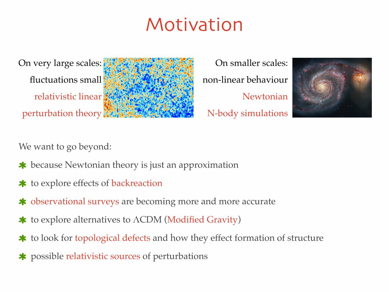
Motivation

We want to go beyond:

because Newtonian theory is just an approximation

to explore effects of backreaction

observational surveys are becoming more and more accurate

to explore alternatives to ΛCDM (Modified Gravity)

to look for topological defects and how they effect formation of structure

possible relativistic sources of perturbations

On very large scales:

fluctuations small

relativistic linear

perturbation theory

On smaller scales:

non-linear behaviour

Newtonian

N-body simulations

The formalism

ds

2 = a

2(⌧)[�(1 + 2 )d⌧2 � 2Bixid⌧ + (1� 2�)�ijdx

idx

j + hijdxidx

j ]

The metric in longitudinal gauge:

Green and Wald: arXiv:1011.4920, 1111.2997

Adamek et al: arXiv:1408.3352

Example: we keep terms:

gravitational potentials are ~10-5

gradients related to peculiar velocities and therefore ~10-3

second spatial derivatives: non perturbative

galactic and cluster scales

Approximation:

every metric perturbation ~ ε every spatial derivative ~ ε-1/2

⇠ �

⇠ �,i�,j or ��,ij

}

“the weak-field limit“, but with spatial derivatives up to all orders

Equations of motion:

(from the time-time part)

(from the transverse-traceless spatial part)

Where the energy-momentum tensor is given by:

T

µ⌫ =X

n

m(n)�

(3)(x� x(n))p�g

�g↵�

dx↵(n)

d⌧

dx�(n)

d⌧

!�1/2dxµ

(n)

d⌧

dx⌫(n)

d⌧

and: ⇧ij = �ikTkj � 1

3�ijT

kk

Adamek et al: arXiv:1408.3352

Post-Newtonian estimation has been used to probe relativistic effects:

using the output of a 3D purely Newtonian simulation (Gadget 2)

(�� )Bi

hij

ds

2 = a

2(⌧)[�(1 + 2 )d⌧2 � 2Bixid⌧ + (1� 2�)�ijdx

idx

j + hijdxidx

j ]

Toy model: spherical symmetryMotivation:

Spherical metric:

simplifies the equations to solve

much faster compared to the full 3D simulation

you can run many simulations for different configurations

easy to compare to the analytical solution

in addition, useful to model e.g. expansion of a void

ds2 = �a2(⌧)⇥(1 + 2 (⌧, r)) d⌧2 + (1� 2�(⌧, r))

�dr2 + r2d⌦2

�⇤

metric perturbations depend only on radial coordinate

and comoving time

particles are pressureless “spherically symmetric shells”

�,rr +2

r�,r � 3H�,⌧ � 3H2(�� �) +

3

2(�,r)

2 = �4⇡Ga2(1� 4�)�T 00

The Einstein equations:

From we get:

From , the traceless part of the

“space-space” component we get :

G00 = 8⇡GT 0

0

Gij �

1

3�ijG

kk = 8⇡G

✓T ij �

1

3�ijT

kk

◆

�,rr �1

r�,r + �2

,r + 2�2,r + 2

✓�,rr �

1

r�,r

◆(2�� �) = 12⇡Ga2(1� 2�)⇧rr

� = �� where⇧ij = �ikTkj � 1

3�ijT

kk

We define the covariant momentum:

p =(1� �)

�drd⌧

�q

1 + 2 � (1� 2�)�drd⌧

�2dp

d⌧= �(H� �,⌧ )p� ,r

p1 + p2

from the geodesic equation velocities don’t need to be small!

Discretisation In order to solve Einstein’s equations numerically we need to discretise them.

The spatial domain is divided into n comoving “grid-cells”

Fields live on the grid-cells

Energy-momentum tensor lives in the grid cells

Particles live in “continuous” space

We need to establish a correspondence between the two

Particle-to-mesh projection: cloud-in-cell, triangular …

Interpolation of fields to propagate particles.

On each step of the simulation we:

1) project particles’ positions to the grid to determine the density and energy-

momentum tensor at each grid cell using particle-to-mesh projection

2) discretise EOM and solve for potential and

3) update particles’ momenta using geodesic equation:

4) evolve particles’ positions using:

5) evolve the background:

Steps 3-5 are done simultaneously, using Runge-Kutta 4.

�

dp

d⌧= �(H� �,⌧ )p� ,r

p1 + p2

dr

d⌧=

pp1 + p2

(1 + �+ )

H2 =8⇡G(⇢+ ⇤)

3

Initial conditions

0.9991

1.005

r

rêr

0.995

11.001

r

rêroverdensity “void”

In the full 3D simulation:

To test our spherically symmetric case:Compensated top-hat profiles.

the Zel’dovich approximation

2LPT

An overdensityResults: testing the code

0.0 0.2 0.4 0.6 0.8 1.0

1.00

1.05

1.10

1.15

1.20

1.25

1.30

1.35

r

rêr

0.0 0.2 0.4 0.6 0.8 1.0

-8.¥10-10

-6.¥10-10

-4.¥10-10

-2.¥10-10

0

r

c=F-Y

0.0 0.2 0.4 0.6 0.8 1.0

-0.000025

-0.00002

-0.000015

-0.00001

-5.¥10-6

0

r

F

0.0 0.2 0.4 0.6 0.8 1.0-0.005

-0.004

-0.003

-0.002

-0.001

0.000

r

momentumHpL

phase - space portrait

difference of the potentials

potential

density

An underdensity (void)phase - space portrait:shell crossing

0.0 0.2 0.4 0.6 0.8 1.0

0.5

1.0

1.5

r

rêr

0.0 0.2 0.4 0.6 0.8 1.0

-2.5¥10-10-2.¥10-10-1.5¥10-10-1.¥10-10-5.¥10-11

0

r

c=F-Y

0.0 0.2 0.4 0.6 0.8 1.00

5.¥10-6

0.00001

0.000015

r

F

0.0 0.2 0.4 0.6 0.8 1.00.0000

0.0005

0.0010

0.0015

0.0020

r

momentumHpL

difference of the potentials

potential

density

Fields need to be weak, but density contrast doesn’t!

Comparison to the LTB solutionWe want to compare our results to analytical Lemaitre-Tolman-Bondi (LTB) solution

ds2 = �dt2 +(@rR(t, r))2

(1 + 2E(r))dr2 +R2(t, r)d⌦2

R(t, r) = �M(r)(1� cos ⌘)

2E(r)(⌘ � sin ⌘)2/3 = �2E(r)t2/3

M(r)2/3

The metric:

Solutions:

Where M(r) is just the mass within the radius r.

Specifically, with our top-hat initial conditions, we get:

r < r1

r1 < r < r2

Initially, we can perform a linear gauge transformation between LTB and our metricAt later times linearity breaks down so we can no longer compare the two solutions. Instead, we can compare gauge independent variables

E(r) ! �10a2in�1r2

27t2in

E(r) ! �10a2in

��2r3 + �1r31 � �2r31

�

27rt2in

Observables1) Redshift of an in-falling source

We track a ray of light, emitted at the boundary of top-hat overdensity through the simulation volume and “absorb” it at the other end To propagate the ray, simulation update step is sub-divided into n smaller steps: this is defined by the courant factor which sets the resolution in time

1 + z =(g

µ⌫

kµu⌫)|src

(gµ⌫

kµu⌫)|obs

the redshift:

gµ⌫kµu⌫ = �k0a[�(1� �� ( + �)p2)p

+(1 + � ( + �)p2)p

1 + p2]

From the null-shell condition (ds2=0) and geodesic equation you get:

dr

d⌧= ± (1 + + �) , d'

d⌧= 0

dk0

d⌧+

,⌧ ��,⌧ +2 ,r

✓dr

d⌧

◆+ 2H

�k0 = 0

LTB

Numerical

0.0 0.2 0.4 0.6 0.80.00

0.02

0.04

0.06

0.08

a

z

2) Lensing of non-radial rays (on an overdensity)

We solve the geodesic equation for number of rays incoming at different angles:

0 20 40 60 800.00000

0.00005

0.00010

0.00015

0.00020

incoming angle

deflection

Comparison to the Schwarzschild solutionMotivation: independent test of our numerical scheme Equations:

Compared to Newtonian solution

Compared to relativistic numerical sol

In post-Newtonian counting our numerical scheme is one orderbetter than purely Newtonian.

Schwarzschild metric in isotropic coordinatesds2 = �

�1� rS

4r

�2�1 + rS

4r

�2 dt2 +

⇣1 +

rS4r

⌘4 ⇥dr2 + r2d⌦2

⇤

Expansion for r >> rs:�1� rS

4r

�2�1 + rS

4r

�2 = 1 + 2 (r) = 1� rSr

+r2S2r2

+ . . .

⇣1 +

rS4r

⌘4= 1� 2�(r) = 1 +

rSr

+3r2S8r2

+ . . .

vacuum stationary solution

� = �GM/r

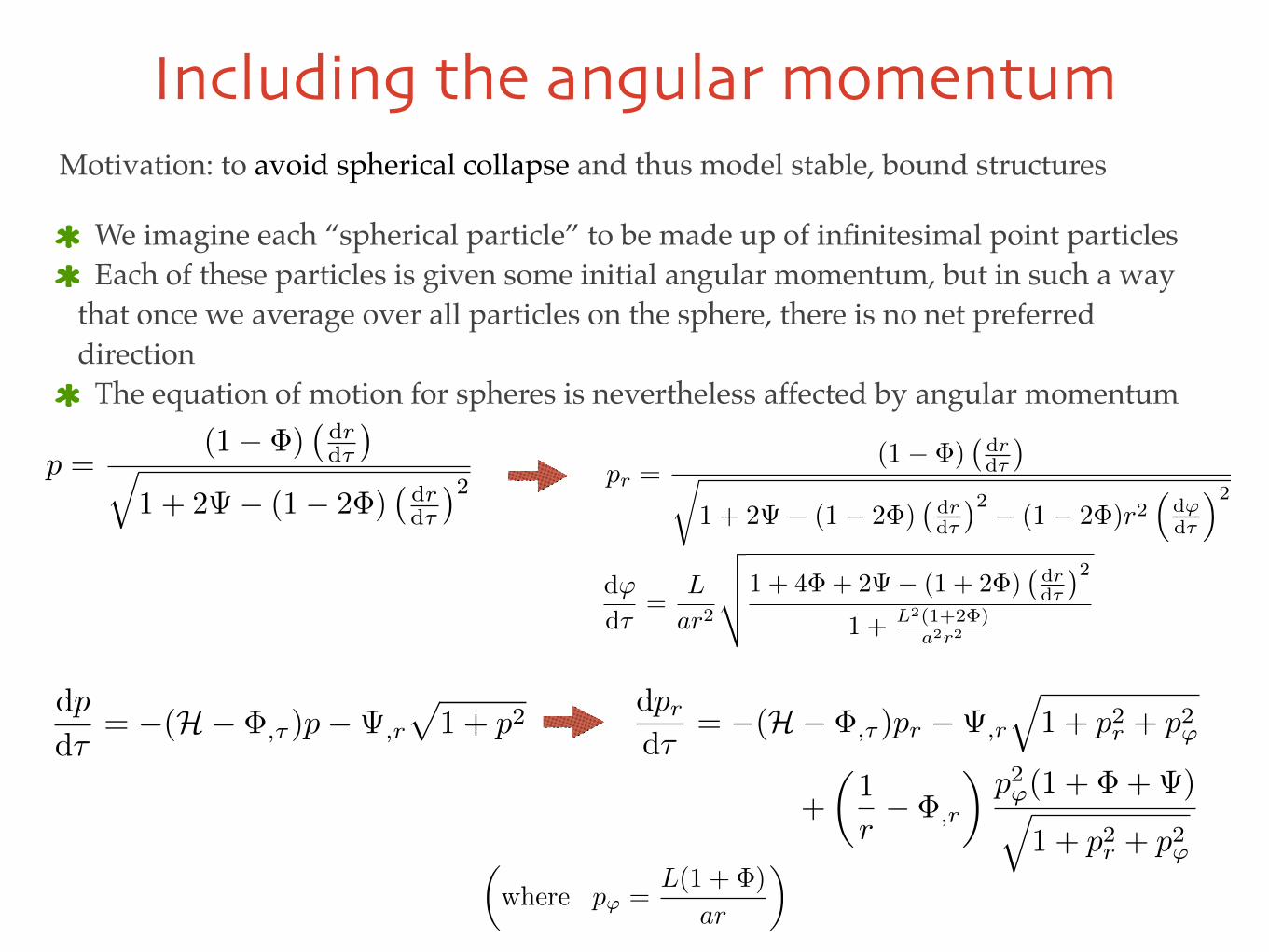
Including the angular momentum

pr =(1� �)

�drd⌧

�r

1 + 2 � (1� 2�)�drd⌧

�2 � (1� 2�)r2⇣

d'd⌧

⌘2p =

(1� �)�drd⌧

�q

1 + 2 � (1� 2�)�drd⌧

�2

We imagine each “spherical particle” to be made up of infinitesimal point particles Each of these particles is given some initial angular momentum, but in such a way that once we average over all particles on the sphere, there is no net preferred direction The equation of motion for spheres is nevertheless affected by angular momentum

Motivation: to avoid spherical collapse and thus model stable, bound structures

d'

d⌧=

L

ar2

vuut1 + 4�+ 2 � (1 + 2�)�drd⌧

�2

1 + L2(1+2�)a2r2

dp

d⌧= �(H� �,⌧ )p� ,r

p1 + p2

dprd⌧

= �(H� �,⌧ )pr � ,r

q1 + p2r + p2'

+

✓1

r� �,r

◆p2'(1 + �+ )q1 + p2r + p2'✓

where p' =L(1 + �)

ar

◆

Conclusions and future applications We implemented a general relativistic approximations that requires weak-field limit,

but allows large gradients of the fields and arbitrarily large velocities of particles

Spherical symmetry makes numerical solving simple and fast

Comparing our results to the analytical LTB solution we find good agreement

Comparing to Schwarzschild solution we find the approximation to be at the post-

Newtonian level of accuracy

In addition, our code can handle shell-crossing

Although spherical symmetry hides vector and tensor perturbations, one can still use

our approach to explore relativistic effects due to the difference of the potentials

In the future we want to: explore the effects of modified gravity or quintessence-type scalar field theory statistical study of properties of environments that allow creation of primordial black holes in the early universe

Thank you!