1 Construction and Encoding of QC-LDPC Codes Using Group Rings Hassan Khodaiemehr and Dariush Kiani Abstract Quasi-cyclic (QC) low-density parity-check (LDPC) codes which are known as QC-LDPC codes, have many applications due to their simple encoding implementation by means of cyclic shift registers. In this paper, we construct QC-LDPC codes from group rings. A group ring is a free module (at the same time a ring) constructed in a natural way from any given ring and any given group. We present a structure based on the elements of a group ring for constructing QC-LDPC codes. Some of the previously addressed methods for constructing QC-LDPC codes based on finite fields are special cases of the proposed construction method. The constructed QC-LDPC codes perform very well over the additive white Gaussian noise (AWGN) channel with iterative decoding in terms of bit-error probability and block-error probability. Simulation results demonstrate that the proposed codes have competitive performance in comparison with the similar existing LDPC codes. Finally, we propose a new encoding method for the proposed group ring based QC-LDPC codes that can be implemented faster than the current encoding methods. The encoding complexity of the proposed method is analyzed mathematically, and indicates a significate reduction in the required number of operations, even when compared to the available efficient encoding methods that have linear time and space complexities. Index Terms Group rings, low-density parity-check (LDPC) codes, quasi-cyclic (QC) codes I. I NTRODUCTION H. Khodaiemehr and D. Kiani are with the Department of Mathematics and Computer Science, Amirkabir University of Technology (Tehran Polytechnic), Tehran, Iran (emails: [email protected] and [email protected]). D. Kiani is also with the School of Mathematics, Institute for Research in Fundamental Sciences (IPM), P.O. Box 19395-5746, Tehran, Iran. arXiv:1701.00210v1 [cs.IT] 1 Jan 2017
Transcript
1
Construction and Encoding of QC-LDPC
Codes Using Group Rings
Hassan Khodaiemehr and Dariush Kiani
Abstract
Quasi-cyclic (QC) low-density parity-check (LDPC) codes which are known as QC-LDPC codes,
have many applications due to their simple encoding implementation by means of cyclic shift registers.
In this paper, we construct QC-LDPC codes from group rings. A group ring is a free module (at the
same time a ring) constructed in a natural way from any given ring and any given group. We present
a structure based on the elements of a group ring for constructing QC-LDPC codes. Some of the
previously addressed methods for constructing QC-LDPC codes based on finite fields are special cases
of the proposed construction method. The constructed QC-LDPC codes perform very well over the
additive white Gaussian noise (AWGN) channel with iterative decoding in terms of bit-error probability
and block-error probability. Simulation results demonstrate that the proposed codes have competitive
performance in comparison with the similar existing LDPC codes. Finally, we propose a new encoding
method for the proposed group ring based QC-LDPC codes that can be implemented faster than the
current encoding methods. The encoding complexity of the proposed method is analyzed mathematically,
and indicates a significate reduction in the required number of operations, even when compared to the
available efficient encoding methods that have linear time and space complexities.
Index Terms
Group rings, low-density parity-check (LDPC) codes, quasi-cyclic (QC) codes
I. INTRODUCTION
H. Khodaiemehr and D. Kiani are with the Department of Mathematics and Computer Science, Amirkabir University of
The identity element 1G of G induces a canonical embedding of the coefficient ring Fq into FqG
and the multiplicative identity element of FqG is (1)1G where the first 1 comes from Fq and the
second from G. The additive identity element is zero. �
A. Group rings and the ring of matrices
From now on, we only consider group algebras over a finite group, which are denoted by G
and H in most cases. Let {g1, g2, . . . , gn} be a fixed listing of the elements of G. We have the
following definition from [26].
6
Definition 1: The RG-matrix of an element w =∑n
i=1 αgigi in the group ring RG is an
element in Mn(R), the ring of n× n matrices over R, defined as
M(RG,w) =
αg−1
1 g1αg−1
1 g2· · · αg−1
1 gn
αg−12 g1
αg−12 g2
· · · αg−12 gn
...... . . . ...
αg−1n g1
αg−1n g2
· · · αg−1n gn
. (2)
It is obvious that each row and each column is a permutation, determined by the group multi-
plication, of the initial row.
Theorem 1 ([23, Theorem 1]): Given a listing of the elements of a group G of order n, there
is a bijective ring homomorphism σ : w 7→M(RG,w) between RG and the RG-matrices over
R.
III. DEFINITIONS AND BASIC CONCEPTS OF QUASI-CYCLIC LDPC CODES
Let t and b be two positive integers. A b× b circulant is a b× b matrix for which each row is
a right cyclic-shift of the row above it and the first row is the right cyclic-shift of the last row.
The top row (or the leftmost column) of a circulant is called the generator of the circulant. A
binary QC code Cqc is commonly specified by a parity-check matrix, which is a (t− c)× t array
of b× b circulants over F2.
A. Construction of QC-LDPC codes based on finite fields
Consider the Galois field Fq, where q is a power of a prime number p. Let α be a primitive
element of Fq. Then, {α−∞ = 0, α0 = 1, α. · · · , αq−2} form all the q elements of Fq. For each
nonzero element αi, with 0 ≤ i < q−1, we define a (q−1)-tuple over F2, z(αi) = (z0, . . . , zq−2),
where the ith component zi is 1 and all the other q − 2 components are set to zero. The binary
vector, z(αi), is referred to as the location-vector of αi, with respect to the multiplicative group
of Fq, or the M -location-vector of αi. The location-vector of the 0 element of Fq is defined as
the all-zero (q − 1)-tuple, (0, 0, . . . , 0).
For a given δ ∈ Fq, we form a (q−1)× (q−1) matrix A over F2 with the M -location-vectors
of δ, αδ, . . . αq−2δ as the rows. Then, A is a (q − 1) × (q − 1) circulant permutation matrix
(CPM), i.e., A is a permutation matrix for which each row is the right cyclic-shift of the row
above it and the first row is the right cyclic-shift of the last row. The matrix A is referred to as
the (q−1)-fold matrix dispersion (or expansion) of the field element δ over F2. The construction
7
of the parity-check matrices of the QC-LDPC codes starts with an m × n matrix W over Fqgiven by
W =[
Wt0 Wt
1 · · · Wtm−1
]t
=
w0,0 w0,1 · · · w0,n−1
w1,0 w1,1 · · · w1,n−1
...... . . . ...
wm−1,0 wm−1,1 . . . wm−1,n−1
, (3)
whose rows satisfy the following two constraints:
1) for 0 ≤ i < m and 0 ≤ k, l < q−1, with k 6= l, αkWi and αlWi have at most one position
in which both of them have the same symbol from Fq (i.e., they differ in at least n − 1
positions);
2) for 0 ≤ i, j < m, and i 6= j, with 0 ≤ k, l < q− 1, αkWi and αlWj differ in at least n− 1
positions.
The above two constraints on the rows of the matrix W are referred to as α-multiplied row
constraints 1 and 2, respectively. These conditions are the sufficient conditions or the design
criteria [19] for constructing the parity-check matrix of the QC-LDPC codes. In order to complete
the construction, it is enough to replace each entry of W by its (q − 1)-fold matrix dispersion
over F2. For an m × n matrix W over Fq, in which the entries are written as the powers of
the primitive element α of Fq, we define the base matrix or the exponent matrix as the m× nmatrix B over {−∞, 0, 1, . . . , q − 2}, so that Bi,j = λ, for 1 ≤ i ≤ m and 1 ≤ j ≤ n, if and
only if Wi,j = αλ. To simplify the notation, the matrices B and W can be used interchangeably
in the construction of codes.
IV. CONSTRUCTION OF QC-LDPC CODES BASED ON DIFFERENCE SETS AND CYCLIC
GROUP ALGEBRAS
In this section, we present our key theorem based on the notation used in the preceding
sections.
Theorem 2: Let G = {g0 = 1G, g1, g2, . . . gm} be a finite group and Fq be the finite field
of order 2m+1, with primitive element α. Then, the FqG-matrix corresponding to the element
w =∑m
i=0 α2igi gives an (m+ 1)× (m+ 1) matrix W that satisfies the α-multiplied constraints
8
1 and 2. Replacing each component of W by its corresponding (q − 1) × (q − 1) CPM in Fqgives the parity-check matrix of a QC-LDPC code.
Proof: Let W be the corresponding RG-matrix of w and let W0 =[α α2 α4 · · · α2m
]be its first row. We can consider the other rows as permutations of the first row. Thus, if we
check the constraint 1 for W0, the other rows also fulfill the constraint 1. Let 0 ≤ k, l < q − 1,
be two integers, with k 6= l, and consider the vectors αkW0 and αlW0. Then, having the same
values in position i1 is equivalent to 2i1 +k = 2i1 + l that implies k = l, which is a contradiction.
Now, we check the second condition. Consider two different permutations of W0 as follows
Wi =[α2i0 α2i1 · · · α2im
]Wj =
[α2j0 α2j1 · · · α2jm
].
Without loss of generality, assume αkWi and αlWj have the same values in the first and second
positions. Then,
2i0 + k = 2j0 + l, i0 6= j0,
2i1 + k = 2j1 + l, i1 6= j1.
Consequently, 2i0 +2j1 = 2j0 +2i1 , where i0 6= i1 and j0 6= j1. We consider three different cases.
Case 1: If i0 < j1, then
2i0(1 + 2j1−i0) =
2i1(1 + 2j0−i1), i1 < j0
2j0(1 + 2i1−j0), i1 > j0
2j0+1, i1 = j0.
The first equation implies i0 = i1, which is a contradiction. Using the second equation we
conclude that i0 = j0 and j1− i0 = i1− j0, which implies that i1 = j1. Thus, k = l which is a
contradiction. Now we consider the third equation. In the left side of this equation we have a
product of an even and an odd number and in the right side we have an even number. The only
possibility is to have j1 = i0 and i0 + 1 = j0 + 1, that imply j0 = j1, which is a contradiction.
Case 2: If i0 = j1, we can show conveniently that i1 = j0 and the equation 2i0−2i1 = 2i1−2i0
leads to a contradiction.
Case 3: If i0 > j1, the proof is the same as the first case.
Thus, W fulfills the α-multiplied constraints 1 and 2.
It follows from Theorem 2 that the Tanner graph associated with the matrix W has girth at
least 6.
9
Theorem 2 is also valid for other prime numbers instead of 2. Now, we present some examples
using the construction method of Theorem 2.
Example 2: We consider the groups of order 8 which give the codes of length 8×255 = 2040.
The groups with 8 elements are Z8, Z2 × Z2 × Z2, Q8, D8 and Z2 × Z4. We represent the
corresponding matrix of the element w in Theorem 2 by a matrix that contains the powers of
α, which is referred to as the exponent matrix. For example, Wij = 2 for 1 ≤ i, j ≤ 8, means
Wij = α2, where α is the primitive element of F28 . The F28Z8-matrix of w in Theorem 2 is as
follows
WF28Z8 =
1 2 4 8 16 32 64 128
128 1 2 4 8 16 32 64
64 128 1 2 4 8 16 32
32 64 128 1 2 4 8 16
16 32 64 128 1 2 4 8
8 16 32 64 128 1 2 4
4 8 16 32 64 128 1 2
2 4 8 16 32 64 128 1
. (4)
If we consider G = D8, the dihedral group of order 8, which is defined as
D8 = 〈r, s|r4 = 1, s2 = 1, s−1rs = r−1〉,
then the F28D8-matrix of w is
WF28D8 =
1 2 4 8 16 32 64 128
8 1 2 4 128 16 32 64
4 8 1 2 64 128 16 32
2 4 8 1 32 64 128 16
16 32 64 128 1 2 4 8
128 16 32 64 8 1 2 4
64 128 16 32 4 8 1 2
32 64 128 16 2 4 8 1
. (5)
The last example that we present here is the quaternion group. The quaternion group is a non-
Abelian group of order eight which is denoted by Q or Q8, and is given by the following group
where 1, the identity element of the group, and −1 commute with the other elements of the
group. The F28Q8-matrix of w is
WF28Q8 =
1 2 4 8 16 32 64 128
2 1 8 4 32 16 128 64
8 4 1 2 128 64 16 32
4 8 2 1 64 128 32 16
32 16 64 128 1 2 8 4
16 32 128 64 2 1 4 8
128 64 32 16 4 8 1 2
64 128 16 32 8 4 2 1
. (6)
By replacing each element of the matrices given in (4), (5) and (6), with their corresponding
CPMs and choosing some rows of the obtained binary matrices, we get regular QC-LDPC codes,
as the null space of these matrices, with different rates and with girth at least 6. �
In order to increase the rate of the constructed codes based on group algebras, we replace
the set of powers in Theorem 2, which is a set of the form{
1, 2, . . . , 2|G|−1}
for a group G, by
other sets that are introduced in the next section.
V. AN ALGEBRAIC FRAMEWORK FOR CONSTRUCTING QC-LDPC CODES BASED ON
GROUP RINGS
In this section, we generalize the construction of Section IV and relate the design of a QC-
LDPC code to the selection of two elements in two different group rings. Let G be a group
of order v′. A k′-subset D of G is a (v′, k′, λ)-difference set if the list of differences d1d−12 ,
d1, d2 ∈ D, contains each non-identity element of G exactly λ times. The number n′ = k′ − λis the order of the difference set. A difference set D in G is non-Abelian, Abelian or cyclic
provided G is non-Abelian, Abelian or cyclic, respectively. The difference sets can be defined
by using an algebraic approach.
Let F be a field and G be a multiplicative group. A subset D ⊆ G is identified with an
element D =∑
g∈D g ∈ FG. Moreover, D(−1) =∑
g∈D g−1.
Theorem 3 ([27, Theorem 18.19]): A k′-subset D ⊆ G of a group G of order v′ with identity
element 1G is a (v′, k′, λ)-difference set of order n′, if and only if D ·D(−1) = n′ · 1G + λ · Gin CG.
11
In the construction of QC-LDPC codes, we need difference sets with λ = 1 to avoid 4-cycles
in the Tanner graph of the code. Let G and H be two finite Abelian groups. In the sequel,
we introduce a new ring R, which is related to H , and the construction of QC-LDPC codes
using the elements of the group algebra RG. Let d =∑
h∈D h ∈ CH be an element satisfying
Theorem 3. Consider D = {d1, d2, . . . , dk′} as the set of indices that appear in d, which is a
subset of H . Then, we define an element w in RG and proceed like Theorem 2. It should be
noted that both G and H can affect the performance of the constructed code, as will be shown
in the simulation results. The structure of the group G can also affect the encoding complexity.
A. Construction of group ring based QC-LDPC codes using cyclic groups
The first and the obvious case is to consider both G and H as cyclic groups. The existence and
the construction of the appropriate difference sets, in some classes of cyclic groups, is guarantied
by using the following theorems.
Theorem 4 ([27, Construction 18.28]): Let α be the generator of the multiplicative group of
Fqm . Then, the set of integers{
0 ≤ i < qm−1q−1
: tracem/1(αi) = 0}
modulo (qm − 1)/(q − 1)
forms a (cyclic) difference set with parameters(qm − 1
q − 1,qm−1 − 1
q − 1,qm−2 − 1
q − 1
). (7)
Here, the trace denotes the usual trace function tracem/1(β) =∑m−1
i=0 βqi from Fqm onto Fq .
These difference sets are Singer difference sets.
Theorem 5 ([27, Construction 18.29]): Let f(x) = xm+∑m
i=1 aixm−i be a primitive polynomial
of degree m in Fq. Consider the recurrence relation γn = −∑mi=1 aiγn−i and take arbitrary start
values. Then the set of integers{
0 ≤ i < qm−1q−1
: γi = 0}
is a Singer difference set.
By using Theorem 4 and 5, we can construct a (q2 + q + 1, q + 1, 1)-difference set in the
additive group Zq2+q+1, when q is a power of a prime number. The constructed codes in this
case are just the same as the constructed codes in [28]. The authors of [28], have proposed
the construction of 4-cycle free QC-LDPC codes using the cyclic difference sets. For a given
difference set D = {d1, d2, . . . , dk′} in Zv′ , with d1 < d2 < · · · < dk′ , they considered the finite
field Fq in 3 different cases: q = v′ + 1, or q ≥ 2dk′ + 1 or q ≥ 2dk′−1 + 1. The table of the
difference sets with small parameters, is available in [27, pp. 427–430], which can be used in
the construction of QC-LDPC codes as above.
12
Now, we consider the general case where the group H is non-cyclic. As we saw in Section
IV, the structure of G has no effect on our design procedure and our concentration here is on
the structure of H . Hence, to simplify, we assume that G is a cyclic group. Let H be an Abelian
group. We have the following theorem for Abelian groups.
Theorem 6 ([29, p. 193]): Every finite Abelian group H is isomorphic to a direct product of
cyclic groups of the form
Zpβ11× Z
pβ22× · · · × Z
pβtt,
where pi’s are primes (not necessarily distinct) and βi’s are some positive integers.
We can see from the proof of Theorem 2 that existence of a difference set in H , is not
necessary for constructing QC-LDPC codes and we can replace this assumption by a weaker
condition. In the next section, we introduce a new method for constructing QC-LDPC codes
using Abelian groups.
VI. CONSTRUCTION OF GROUP RING BASED QC-LDPC CODES USING NON-CYCLIC
ABELIAN GROUPS
In [28], QC-LDPC codes were constructed based on difference sets in cyclic groups. Difference
sets do not exist in every cyclic group and furthermore, there is no efficient algorithm to find
them. Thus, the rate and length of the constructed codes based on cyclic difference sets will be
limited. In this section, we introduce some combinatorial structures in arbitrary Abelian groups,
which are close to difference sets and also enough for our application in the construction of
QC-LDPC codes. Then, we propose a new method to construct QC-LDPC codes based on the
proposed structures and the group algebras. As we see in the sequel, these structures give codes
with the highest possible rate of a given length.
A. Combinatorial structures beyond the difference sets in the construction of QC-LDPC codes
In the construction of QC-LDPC codes based on Abelian groups, the first candidates are
difference sets in the Abelian groups. If instead of Zv′ , we consider a group A with v′ elements,
which is written multiplicatively, the condition for a set D ⊂ A with k′ distinct elements to be a
difference set is exactly like the cyclic case. While much is known about the difference sets in
the cyclic groups, little systematic work has been done for non-cyclic groups. As in the cyclic
case, we are interested in difference sets with λ = 1. We say that two difference sets D and
13
D′ in A are equivalent if there exists an automorphism τ of A and an element g ∈ A such that
D′ = Dτg. Non-cyclic difference sets for k′ < 20, are enumerated in [30]. We have summarized
non-equivalent and non-cyclic difference sets, which are proper for the construction of QC-LDPC
codes, in TABLE I. We can see from TABLE I that none of the non-cyclic difference sets with
TABLE I
NON-CYCLIC DIFFERENCE SETS OF SIZE LESS THAN 20
(v′, k′, λ) Underlying group Difference set D
(21, 5, 1) a7 = b3 = 1, ba = a2b 1, a, a3, b, a2b
(57, 8, 1) a19 = b3 = 1, ba = a7b 1, a, a3, a8, b, a4b, a13b,
a18b2
(57, 8, 1) a19 = b3 = 1, ba = a7b 1, a, a3, a8, b, a5b2, a9b2,
a18b2
(183, 14, 1) a61 = b3 = 1, ba = a13b 1, a, a3, a20, a26, a48, a57, b,
a8b, a18b, a29b, a17b2, a32b2,
a44b2
(183, 14, 1) a61 = b3 = 1, ba = a13b 1, a, a3, a20, a26, a48, a57, b,
in which ⊗ denotes the the Kronecker product2 of matrices, the matrix CPM(αijj ,Fqj), for
1 ≤ j ≤ t, is a (qj − 1)× (qj − 1) circulant matrix and its first row is the location-vector of the
element αijj with respect to the multiplicative group of Fqj . We denote the zero element of Fqjby α−∞j . If for some 1 ≤ j ≤ t in (11), ij = −∞, then QCPM(α(i1,...,it)) is defined as the b× bzero matrix.
Example 3: We want to obtain the QCPM of α(1,3) in F4 × F5, which is a 12× 12 matrix as
follows
QCPM(α(1,3)) = CPM(α1,F4)⊗ CPM(α32,F5)
=
0 1 0
0 0 1
1 0 0
⊗
0 0 0 1
1 0 0 0
0 1 0 0
0 0 1 0
.
By replacing each component ai,j of CPM(α1,F4), with ai,j × CPM(α32,F5), we obtain the
following matrix
QCPM(α(1,3)) =
0 0 0 0 0 0 0 1 0 0 0 0
0 0 0 0 1 0 0 0 0 0 0 0
0 0 0 0 0 1 0 0 0 0 0 0
0 0 0 0 0 0 1 0 0 0 0 0
0 0 0 0 0 0 0 0 0 0 0 1
0 0 0 0 0 0 0 0 1 0 0 0
0 0 0 0 0 0 0 0 0 1 0 0
0 0 0 0 0 0 0 0 0 0 1 0
0 0 0 1 0 0 0 0 0 0 0 0
1 0 0 0 0 0 0 0 0 0 0 0
0 1 0 0 0 0 0 0 0 0 0 0
0 0 1 0 0 0 0 0 0 0 0 0
.
2If A is an m× n matrix and B is a p× q matrix, then the Kronecker product A⊗B is the mp× nq block matrix:
A⊗B =
a1,1B · · · a1,nB
.... . .
...
am,1B · · · am,nB
.
20
�
In order to complete our construction method, we consider the ring R which is formed by the
Z-linear combination of the basis elements of the form αi11 ⊗ · · · ⊗ αitt , where 0 ≤ ij ≤ qj − 2
and 1 ≤ j ≤ t. Alike the previous cases, the construction of QC-LDPC codes from Abelian
group rings needs an m×n matrix over R, whose rows W1, . . . ,Wm, satisfy the following two
constraints:
1) For 0 ≤ i ≤ m− 1 and k = (k1, . . . , kt), l = (l1, . . . , lt) ∈ Zq1−1× · · · ×Zqt−1 with kj 6= lj
and j = 1, . . . , t, the two vectors αkWi and αlWi have at most one position where both
of them have the same symbol from R, (i.e., they differ in at least n− 1 positions).
2) For 0 ≤ i, j ≤ m − 1, i 6= j, and k = (k1, . . . , kt), l = (l1, . . . , lt) ∈ Zq1−1 × · · · × Zqt−1,
the two vectors αkWi and αlWj differ in at least n− 1 positions.
We call these conditions the α-multiplied constraints 1 and 2, respectively. Note that the multi-
plication of αi11 ⊗ · · · ⊗αitt and αj11 ⊗ · · · ⊗αjtt is defined as αk11 ⊗ · · · ⊗αktt , where kr = ir + jr
(mod qr − 1), for 1 ≤ r ≤ t. We also denote αi11 ⊗ · · · ⊗ αitt by α(i1,...,it). Based on the
aforementioned notations and definitions, we have the following theorem.
Theorem 8: Let D = {d0,d2, . . . ,dn−1} be an S2-set in the Abelian group H = Zq1−1 ×· · · ,×Zqt−1, G = {g0 = 1G, g1, g2, · · · gn−1} be a finite group of order n and Fqi be the Galois
field of order qi with the primitive element αi. Let α = (α1, . . . , αt) and consider the ring R
which is formed by Z-linear combination of the basis elements of the form αi11 ⊗ · · · ⊗ αitt ,
where 0 ≤ ij ≤ qj − 2 and 1 ≤ j ≤ t. If (qi − 1)’s, for 1 ≤ i ≤ t, are odd numbers, then the
RG-matrix corresponding to the element of the form w =∑n−1
i=0 αdigi gives an n × n matrix
W that satisfies the α-multiplied constraints 1 and 2. By replacing each component of W by
its corresponding∏t
i=1(qi−1)×∏ti=1(qi−1) QCPM and choosing a subarray of W, we obtain
the parity-check matrix of a 4-cycle free QC-LDPC code.
Proof: Since all the rows W1, . . . ,Wm−1 are obtained from the permutations of the first
row W0, it is enough to show that the first α-multiplied constraint is fulfilled for W0 =
(αd1 ,αd2 , . . . ,αdk). Let k = (k1, . . . , kt), l = (l1, . . . , lt) ∈ Zq1−1 × · · · × Zqt−1, with l 6= k, be
such that αlW0 and αkW0 have more than one position in common. Then, for some 1 ≤ i ≤ n
and 1 ≤ j ≤ n, αlαdi = αkαdi and αlαdj = αkαdj which yield the following equations
l + di = k + di,
l + dj = k + dj.
21
Consequently, it follows that k = l, which is a contradiction. For the second constraint, assume
that αlW0 and αkWi, where 1 ≤ i ≤ m− 1, have more than one position in common. Then,
for some 1 ≤ i < j ≤ n and 1 ≤ i′ < j′ ≤ n, αlαdi = αkαdi′ and αlαdj = αkαdj′ which
imply the following equations
l + di = k + di′ ,
l + dj = k + dj′ .
Thus, we have di − di′ = dj − dj′ . We also know that i 6= i′ and j 6= j′. If i 6= j′ and i′ 6= j,
we get a contradiction with the assumption that D is an S2-set. Note that l 6= k implies that
i 6= i′ and j 6= j′. If i = j′ and i′ 6= j or if i′ = j and i 6= j′ we conclude that 2di = d′i + dj
or 2dj = di + d′j which is a contradiction, since D is an S2-set. If i = j′ and j = i′, we
have 2di = 2dj mod (q1 − 1, . . . , qt − 1), where, di = (di,1, . . . , di,t), dj = (dj,1, . . . , dj,t) and
the mod operation is applied componentwise. Since (qi − 1) is an odd number for 1 ≤ i ≤ t,
it follows that di = dj which is a contradiction. Thus, if we replace the components of W
with their corresponding QCPMs, we obtain the parity-check matrix of a 4-cycle free QC-LDPC
code.
If we remove the repetitive members in the set 2D, then we obtain an S2-set which satisfies
the conditions of Theorem 8 without requiring that (qi − 1)’s should be odd numbers. Similar
to the cyclic case, we present the parity-check matrix of the code by an array which consists
of the powers of QCPMs. For example αi11 ⊗ · · · ⊗ αitt in the parity-check matrix is denoted by
(i1, . . . , it). We present the steps of Theorem 8 in the next example. Although, all the assumptions
of Theorem 8 are not fulfilled in this example, it is a useful example to see our method for
constructing QC-LDPC codes.
Example 4: Consider the Abelian S2-set D = {(0, 0, 0, 0),
(0, 0, 0, 1), (0, 0, 1, 0), (0, 1, 0, 0), (1, 0, 0, 0), (1, 1, 1, 1)} in Z42. There are two groups of order 6,
namely Z6 and S6. Consider G = Z6 as the underling group. The parity-check matrix of the
QC-LDPC code based on Theorem 8, can be constructed by taking some rows of following
22
matrix and replacing its components with their corresponding QCPMs:
If we consider the first three rows of W, then we obtain a QC-LDPC code of length 96 and
rate at least 0.5. �
Using Theorem 8 and the proposed method in [28], for constructing QC-LDPC codes from
cyclic difference sets, we get the following theorem.
Theorem 9: Let D = {d0,d2, . . . ,dn−1} be an S2-set in the Abelian group H = Zq1−1 ×· · · ,×Zqt−1, G = {g0 = 1G, g1, g2, · · · gn−1} be a finite group of order n and Fqi be the Galois
field of order qi with the primitive element αi. Let α = (α1, . . . , αt) and consider the ring R
23
which is formed by Z-linear combination of the basis elements of the form αi11 ⊗· · ·⊗αitt , where
0 ≤ ij ≤ qj − 2 and 1 ≤ j ≤ t. If (qi − 1)’s, for 1 ≤ i ≤ t are odd numbers, (or 2D contains
no repetitive elements), and W and W−1 are the RG-matrices corresponding to the elements
w =∑n−1
i=0 αdigi and w−1 =∑n−1
i=0 α−digi, respectively, then W′ =[
W W−1
]gives an
n× 2n matrix that satisfies the α-multiplied constraints 1 and 2. By replacing each component
of W′ with its corresponding∏t
i=1(qi − 1)×∏ti=1(qi − 1) QCPM and choosing a subarray of
W′, we obtain the parity-check matrix of a 4-cycle free QC-LDPC code.
Proof: Since all the rows W′1, . . . ,W
′m−1 are obtained from the permutations of the first
row W′0, it is enough to show that the first α-multiplied constraint is fulfilled for W′
0 =
(αd1 , . . . ,αdn|α−d1 , . . . ,α−dn). Let k = (k1, . . . , kt) and l = (l1, . . . , lt) in Zq1−1×· · ·×Zqt−1,
with l 6= k, be such that αlW′0 and αkW′
0 have more than one position in common. Based on
Theorem 8, both of these common positions cannot be in the first n positions or in the last n
positions. For some 1 ≤ i ≤ n and n+ 1 ≤ j ≤ 2n, let αlαdi = αkαdi and αlα−dj = αkα−dj
which results in the following equations
l + di = k + di,
l− dj = k− dj.
Consequently, we have k = l, which is a contradiction. For the second constraint, assume that
αlW′0 and αkW′
i, where 1 ≤ i ≤ m − 1, have more than one position in common. Then, for
some 1 ≤ i 6= i′ ≤ n and n+ 1 ≤ j 6= j′ ≤ 2n, αlαdi = αkαdi′ and αlαdj = αkα−dj′ which
results in the following equations
l + di = k + di′ ,
l− dj = k− dj′ .
It follows that di−di′ = d′j−dj . If i 6= j′ and i′ 6= j, we get a contradiction with the assumption
that D is an S2-set. If i = j and i′ 6= j′ or if i′ = j′ and i 6= j we conclude that 2di = d′i + d′j
or 2d′j = di + dj which is a contradiction, since D is an S2-set. If i = j and i′ = j′, we have
2di = 2d′i mod (q1 − 1, . . . , qt − 1). Since (qi − 1) is an odd number for 1 ≤ i ≤ t, di = d′i
which is a contradiction.
To describe the construction of Theorem 9 by group-rings representations, we can use the
following theorem.
24
Theorem 10 ([25, Lemma 3.4]): Let G and H be two groups and let K be a field. Then
K[G]⊗K K[H] ∼= K[G×H].
We can replace the field K in Theorem 10 by any commutative ring with identity. Thus,
the group ring that describes the construction of Theorem 9 is R[G′] = R[C2 × G], where
C2 = {1,−1} is a multiplicative group of order 2. In this case, we have considered the first n
rows of an RG′-matrix.
C. Achievable parameters of the group ring based QC-LDPC codes
Here, we explain the important parameters of the obtained codes using Abelian group rings.
These parameters are compared with the achievable parameters of the other construction methods,
namely the ones based on finite fields. The parameters that we have considered for our analysis
are the length and the rate of the code. We only consider the girth 6 QC-LDPC codes for our
comparisons. First, we consider the construction methods based on finite fields. We conclude
the following result from [36, Corollary 1] and we use it to estimate the values of rate and
length that can be achieved by using the designed QC-LDPC codes based on the finite fields
approaches.
Proposition 2: In constructing a QC-LDPC code with cyclic lifting degree b using an m× nexponent matrix B, with m ≤ n, that does not contain −∞ in the components, a necessary
condition for having a girth at least 6 in the Tanner graph is b ≥ n.
When we apply Proposition 2 to finite field based QC-LDPC codes, we reach the upper bound
n ≤ q − 1 on the row weight of the code. The construction of QC-LDPC codes based on Latin
squares over finite fields, which is proposed in [37], and the proposed construction methods in
[20], achieve this upper bound. Thus, construction of QC-LDPC codes with lengths γ(q − 1)
and rates 1− ργ
is possible, in which q is a prime power and 1 ≤ γ, ρ ≤ q − 1.
As explained above, by using the approaches based on finite fields, the lifting degree b is of
the form pβ − 1, for a prime number p and a positive integer β. For example, the achievable
values of b, which are smaller than 100, are
2 3 4 6 7 8 10 12 15 16 18,
22 24 26 28 31 35 36 40 42 46 48,
52 58 63 66 70 72 78 80 82 88 96.
25
Thus, only 33% of the possible values for b can be achieved by using the approaches based
on finite fields. When we employ the Abelian group rings, the lifting degree b is of the form∏ti=1
(pβii − 1
), in which pi’s are distinct prime numbers and βi’s and t are positive integers.
In this case, the achievable values for b, which are smaller than 100, are
2 3 4 6 7 8 9 10 12 14 15
16 18 21 22 24 27 26 28 30 31 32
35 36 40 42 45 46 48 49 52 54 56
58 60 62 63 64 66 70 72 78 80 81
82 84 88 90 92 93 96 98 ,where the circled values are the ones that cannot be obtained by using the approaches based on
finite fields. This indicates 57% increase in the number of achievable values for b, compared to
the one for finite fields.
Using Theorem 7, we find an upper bound on the row weight of the group ring based QC-LDPC
codes. Let H be an Abelian group used in our construction. Let s(H) denote the cardinality of
the largest S2-set in H , which gives 2s(H) as the maximum achievable row weight of the group
ring based QC-LDPC codes based on H . Then, by using Theorem 7, it follows that
s(H) ≤⌊
3 +√
9− 4(2− hy(H))
2
⌋
=
⌊3 +
√1 + 4hy(H)
2
⌋, (12)
where bxc, for a real number x, denotes the largest integer less than or equal to x and
hy(H) =|H| (n2(H) + 1)
n2(H). (13)
Finding the Abelian groups that achieve this upper bound, is an interesting problem. When |H|is large enough, we can assume hy(H) ≈ |H| and (12) will be an upper bound in terms of |H|.Consequently, construction of QC-LDPC codes with lengths γ
∏ti=1
(pβii − 1
)and rates 1 − ρ
γ
is possible, in which γ, ρ are integers with 1 ≤ γ ≤ 2s(H) and 1 ≤ ρ ≤ s(H), the pi’s are
distinct prime numbers and the βi’s and t are positive integers.
VII. A NEW ENCODING OF QC-LDPC CODES BASED ON THE MULTIPLICATION OF GROUP
ALGEBRAS
In general, the quasi-cyclic codes are encoded by multiplying a message vector m of length
kb by a (kb × nb) generator matrix G, where G is usually in systematic form, i.e., G =
26
[Ikb Pkb×(n−k)b
], where Ikb is the kb × kb identity matrix. There are two difficulties in the
implementation of this encoding procedure. First, the generator matrix G is usually a dense
matrix and requires a large number of memory units, i.e., b2(n− k)k units, to store P. Second,
although the encoding of QC codes can be partially parallelized so that the computation units
are reduced by a factor of b, the total number of symbol operations is still b2(n − k)k, which
is the same as that for general linear codes. In [18], an efficient encoding method has been
proposed for QC-LDPC codes. The authors of [18] computed a generator matrix G with quasi-
cyclic structure benefiting from the quasi-cyclic structure of the parity-check matrix and the
Gaussian elimination method. Another method was proposed in [23] that uses the structure of
group algebras to obtain the generator matrix. This method can be used for the unit elements of
a group algebra. Let w be a unit element in the group algebra RG. Let W be its corresponding
RG-matrix. Then W is an invertible matrix over R. Without loss of generality, we consider the
parity-check matrix H of the code as the first n− k rows of W. We divide the matrices W and
W−1 as follow
In×n = WW−1 =
H(n−k)×n
Jk×n
[ An×(n−k) Bn×k
]
=
H(n−k)×nAn×(n−k) H(n−k)×nBn×k
Jk×nAn×(n−k) Jk×nBn×k
.The above equation gives H(n−k)×nBn×k = 0n−k×k and consequently, it follows that Bt
n×k is a
generator matrix for the given code.
Although, we used the group rings to construct our QC-LDPC codes, our construction method
is completely different from the presented method in [23]. We design our codes over a group
ring RG, where |G| = n. Then, based on the available connection between the RG-matrices in
Mn(R) and the elements of the group ring, we replace the components of the RG-matrix by their
corresponding QCPMs. In both cases that we considered, i.e., when R is a finite field or when R is
the tensor product of multiple fields, the map that sends the elements of R to their corresponding
QCPMs, is a multiplicative group isomorphism. Indeed, it preserves the multiplication but not
necessarily the addition. Thus, we may have QCPM(r1 + r2) 6= QCPM(r1) + QCPM(r2),
for some r1, r2 ∈ R. In fact, an element U in Mn(R) can be invertible in Mn(R) but after
replacing its components with their corresponding QCPMs, the obtained matrix can be a non-
singular binary matrix (i.e., its determinant can be an even number). The idea that we use here
27
is replacing the matrix multiplication in Mnb(F2), where b =∏t
i=1(qi−1), by a convolution like
operation in the group ring R′G, where
R′ =F2[x1]⟨
xq1−11 − 1
⟩ ⊗ · · · ⊗ F2[xt]⟨xqt−1t − 1
⟩ ,and x1, . . . , xt are independent variables. We define the QCPM of xi11 ⊗ · · · ⊗ xitt ∈ R′, where
0 ≤ ij ≤ qj − 2 and 1 ≤ j ≤ t, as QCPM(α(i1,...,it)), which is a b× b matrix.
Theorem 11: A matrix M ∈Mn(R′) is a unit (a zero-divisor) if and only if the matrix which
is obtained by replacing the components of M with their corresponding QCPMs, is a unit (a
zero-divisor) in Mnb(F2).
Proof: The proof follows from the fact that the map Φ that sends xi to a circulant matrix Xi
of size (qi − 1)× (qi − 1) and with the first row of the form (0, 1, 0, . . . , 0), is an isomorphism
between two rings Mn(R′) and Im(Φ) ⊂ Mnb(F2). We define Φ over other elements of R′
naturally.
A. Mathematical description of encoding for group ring based QC-LDPC codes
Let w be an element in the group algebra R′G and W be its corresponding R′G-matrix of
size n× n. Let H be the rb× nb parity-check matrix of a group ring based QC-LDPC code C,
with r < n. The matrix H is obtained by choosing some rows from the array matrix W, which
is denoted by Harr, and replacing the components of Harr by their corresponding QCPMs. The
group ring R′G is a finite ring with identity and w is either a unit or a zero-divisor. Consequently,
W is either a unit matrix or a zero-divisor matrix in Mn(R′). To simplify our notation, we state
the following theorem.
Theorem 12: Let G be a finite Abelian group and R′G be the aforementioned group ring.
Then, R′G is isomorphic to the group algebra F2G′, where G′ = Cq1−1 × · · · × Cqt−1 ×G and
Cqi−1 is the multiplicative cyclic group of order qi − 1, for i = 1, . . . , t.
Proof: The proof follows from the following isomorphisms
F2[xi]
〈xqi−1i − 1〉
∼= F2Cqi−1, i = 1, . . . , t.
Consequently, R′G ∼= (F2Cq1−1 ⊗ · · · ⊗ F2Cqt−1)[G]. Based on Theorem 10, F2Cq1−1 ⊗ · · · ⊗F2Cqt−1 is isomorphic to F2 [Cq1−1 × · · · × Cqt−1]. Let H = Cq1−1 × · · · ×Cqt−1. We show that
28
F2[H][G] is isomorphic to F2[H × G]. To this end, it can be checked easily that the map Φ
which is given by
Φ
(∑g∈G
∑h∈H
α(g,h)(g, h)
)=∑g∈G
βgg,
is an isomorphism between F2[H ×G] and F2[H][G], where βg =∑
h∈H α(g,h)h ∈ Z2[H].
Now, we describe the encoding approach in both cases.
Case 1: Let W be the R′G-matrix of a unit element w ∈ R′G, Harr be a subarray of W and
H be its corresponding (rb × nb) binary matrix after replacing the QCPMs. Consider U and
u as the inverses of W and w in Mn(R′) and R′G, respectively. We want to encode a binary
vector m ∈ Fkb2 , where k = n − r. We divide the input vector m into k sections of size b as
m = (m1, . . . ,mk). Then, we map the following vector to m
i=0 mj,iXΨ−1(i), X = x1 ⊗ · · · ⊗ xt and Ψ is a bijection map from
Zq1−1 × · · · × Zqt−1 to Zb = Z(q1−1)×···×(qt−1), such that
Ψ (i1, . . . , it) =t−1∑j=1
(ij − 1)
(t∏
s=j+1
(qs − 1)
)+ it. (14)
Let Harr be the subarray of W corresponding to the list L ={g−1i1, . . . , g−1
ir
}in G. Consider
the list L′ = G − {gi1 , . . . , gir} = {gj1 , . . . , gjk}, and mL′ =∑k
i=1 mi(x1, . . . , xt)gji . Then,
the encoding of m can be done by using the flowing group ring multiplication c = mL′u and
replacing the components of c with their corresponding QCPM-generators. The QCPM-generator
of an element xi11 ⊗ · · · ⊗ xitt is the vector eq1−1i1⊗ · · · ⊗ eqt−1
it, where e
qj−1ij
is a vector of length
(qj − 1) in which the ithj position is 1 and the other components are 0, for j = 1, . . . , t. We
check the validity of this statement in Theorem 13.
Theorem 13: Let Harr be the subarray of W corresponding to a list L ={g−1i1, . . . , g−1
ir
}in
G, (i.e., Harr is formed by rows i1, . . . , ir of W). If we construct the parity-check matrix of the
code C from Harr, based on [23, Theorem 5.1], the matrix Garr formed by the rows of W−1 with
indices given in L′ = {gj1 , . . . , gjk} = G−{gi1 , . . . , gir}, can be used to construct the generator
matrix of C. Replace the components of Harr and Garr with their corresponding QCPMs and
denote the obtained matrices by H1 and G1, respectively. The encoding of a vector m of length
kb, that means the calculation of mG1, can be done by computing the group ring multiplication
c = mL′u and replacing the components of c with their corresponding QCPM-generators.
29
Proof: The encoding of m = (m1, . . . ,mk), where mi = (mi,0, . . . ,mi,b−1) and i =
1, . . . , k, means the calculation of c = mG1. Using block matrices, we have
c =[
m1 · · · mk
]
W′g−1j1g0· · · W′
g−1j1gn−1
... . . . ...
W′g−1jkg0· · · W′
g−1jkgn−1
, (15)
where W′g−1jzgs
is the QCPM of the (jz, s)th component of W−1. For z = 1, . . . , n, the sub-block
cz, which corresponds to the indices (z−1)b+1 to zb of c, is obtained by(∑k
i=1 miW′g−1jigz
)gz.
The group element gz in the right side of this equation indicates the location of the sub-vector∑ki=1 miW
′g−1jigz
in the given codeword c. In our proposed encoding method, we compute the
group ring multiplication
c =
(k∑i=1
mi(x1, . . . , xt)gji
)(w′g0g0 + · · ·+ w′gn−1
gn−1).
Using the properties of the group ring multiplication, the coefficient of gz in the above multiplica-
tion is∑k
i=1 mi(x1, . . . , xt)gjiw′gkigki , where gjigki = gz, for i = 1, . . . , k. Since G is an Abelian
group, we have gki = g−1jigz and the coefficient of gz is
(∑ki=1 mi(x1, . . . , xt)w
′g−1jigz
)gz. After
replacing the QCPM-generators, we reach the same result as the usual encoding.
Case 2: Let w be a zero divisor in R′G and W ∈ Mn(R′) be its corresponding R′G-
matrix such that for a matrix U ∈ Mn(R′) and u ∈ R′G, WUt = 0n×n and wut = 03.
Let Harr be the subarray of W corresponding to the list L ={g−1i1, . . . , g−1
ir
}⊂ G and H be its
corresponding (rb×nb) binary matrix which is obtained by replacing the elements of Harr with
their corresponding QCPMs. Let C be a code with parity-check matrix H. Then, the generator
matrix of C is a k′ × nb binary matrix such that GHt = 0k′×rb, where k′ = nb − rank(H). If
the matrix H has full rank, then instead of finding the generator matrix of C, we consider H as
the generator matrix of the code C⊥ and we find its parity-check matrix. Similar to the method
used in Theorem 13, every codeword c′ in C⊥ is obtained as follows: first, we have an element
c′ in R′G of the form c′ = mw, where m ∈M ′ and M ′ is the R′-submodule of R′G generated
by the list L of G. Then, the vector c′ is obtained by replacing the components of c′ with
their corresponding QCPM-generators. If Lw is linearly independent, rank(W) = |L| = r and
3For a given group G = {g0 = 1G, g1, . . . , gn−1} and a group ring RG, let u =∑n−1i=0 βgigi be an element in RG. Then
we define ut as∑n−1i=0 βgig
−1i .
30
rank(U) = n−r, then we find n−r independent rows of U which are in accordance with a list
in G like L′ ={g−1j1, . . . , g−1
jn−r
}. We put these n− r independent rows of U in a matrix which
is denoted by Uarr. Then, a necessary and sufficient condition to have a single check element, is
obtaining the rank (n− r)b after replacing the elements of Uarr by their corresponding QCPMs
[23, Theorem 4.9]. Hence, the encoding of a vector m can be done by using the group ring
multiplication c = mL′u, where mL′ =∑n−r
i=1 mi(x1, . . . , xt)gji , and replacing the components
of c with their corresponding QCPM-generators. Now, let both H and Harr have full rank,
dimM ′ = |L| = r < ω = rank(W) and WUt = 0n×n, with rank(U) = n − ω. In addition,
let the substituting of QCPMs in U admit a matrix of rank (n − ω)b. In this case, we obtain
the generator matrix of C by adding ω− r extra vectors to the independent rows of U or Uarr.
Moreover, the rows of W corresponding to the list L of G, are independent and we can extend
L to a subset T ={g−1i1, . . . , g−1
ir, g−1ir+1
, . . . , g−1iω
}of G, corresponding to the independent rows
of W, and put all these row vectors in a matrix Wω. Since, rank(W) = ω, there exists an n×ωmatrix C such that WωC = Iω. This implies
WωC =
Harr
H2
[ C1 C2
]= Iω. (16)
We conclude that HarrC2 = 0r×(ω−r). Let Un−ω be a matrix formed by n−ω linearly independent
columns of U. Then, it can be shown [23], that the binary matrix Gb that is obtained by replacing
the components of Garr =[
Un−ω C2
]twith their corresponding QCPMs, is the generator
matrix of C. In Remark 7.1, we have explained the details of our encoding method based on
multiplication of group rings.
Remark 7.1: Using the aforementioned notation, let the binary matrix Gb of size (n−r)b×nbbe the generator matrix of C obtained from Garr =
[Un−ω C2
]tby replacing its components
with their corresponding QCPMs. Let Un−ω be the subarray of R′G-matrix U corresponding to
the list Lu ={gj1 , . . . , gjn−ω
}⊂ G. Let Ub
n−ω and Cb2 be the matrices obtained by replacing
the QCPMs in Un−ω and C2, respectively. The encoding of m = (m1, . . . ,mk), with mi =
(mi,0, . . . ,mi,b−1), i = 1, . . . , k and k = n− r, can be done as c = mGb, which is equivalent to
c = m1Ubn−ω + m2Cb
2, (17)
where m1 = (m1, . . . ,mn−ω) and m2 = (mn−ω+1, . . . ,mk). Since Un−ω is a subarray of the
R′G-matrix U, by using the same method in the proof of Theorem 13, we can prove that the
31
term c1 = m1Ubn−ω can be obtained by performing the following group ring multiplication
c1 =
(n−ω∑i=1
mi(x1, . . . , xt)g−1ji
)(utg0g0 + · · ·+ utgn−1
gn−1),
where (utg0 , . . . , utgn−1
)t is the first column of U. It is enough to show that the term c2 = m2Cb2
can also be obtained by using a group ring multiplication. To this end, C2 must be a subarray
of an R′G-matrix. Let us consider WωC = Iω and let C1 be the first column of C. Let W1 be
the first row of the R′G-matrix W. Since all other rows of W can be written as a permutation
of the first row, Wω will be of the following form
Wω =
g−1i1
(W1)...
g−1iω
(W1)
, (18)
where g−1ij
(W1), for j = 1, . . . , ω, is the ithj row of W. Note that WωC = Iω implies⟨g−1ij
(W1), (C1)t⟩
= δj,1, for j = 1, . . . , t, in which δj,1 = 1 (j = 1), 0 (j 6= 1) is the
Keronecker’s delta and 〈, 〉 denotes the inner product in Fn2 . We also have the following trivial
result.
Lemma 14: Let F be an arbitrary field and let 〈, 〉 denote the inner product over Fn, for a
positive integer n. Then, for every x,y ∈ Fn, and every permutation σ on {1, . . . , n}, 〈x,y〉 =
〈σ(x), σ(y)〉.If there exists a set I = {g1, . . . , gω} ⊂ G such that g−1
l g−1is∈ T =
{g−1i1, . . . , g−1
ir, g−1ir+1
, . . . , g−1iω
},
for l, s = 1, . . . , ω, then based on Lemma 14, there exists a reordering on I, like {g′1, . . . , g′ω},that gives an R′G-matrix C′ as
C′ =[g′1(C1) · · · g′ω(C1)
],
such that WωC′ = Iω. Thus, instead of C2, we can consider a submatrix of C′ which is an R′G
matrix. Consequently, the second part of encoding, i.e., m2Cb2, can be obtained by substituting
the QCPM-generators in the components of the following group ring multiplication
c2 =
(n−r∑
i=n−ω+1
mi(x1, . . . , xt)(g′i+ω−n+r)
−1
)c′R′G, (19)
where c′R′G = C ′1,1g0 + · · · + C ′n,1gn−1 and (C ′1,1, . . . , C′n,1)t is the first column of C′. In this
case, the codewords of C cannot be obtained by using a single generator. Removing each one
of the aforementioned conditions makes the encoding highly complicated. �
32
Due to the mathematical complexity of the encoding method proposed in Case 2, finding an
elements w in R′G that satisfy the assumptions of Case 1 is our desire. In Proposition 3, we
specify some conditions under which the obtained array matrix W, remains an invertible matrix
over F2 after replacing the components of W with their corresponding QCPMs. We need the
following results and definitions to establish this result.
Let Γ denote the n× n cyclic shift matrix whose entries are Γi,j = 1 if j − i ≡ 1 (mod n),
and 0, otherwise. An n × n circulant matrix A over the ring of integers modulo m, which is
denoted by Zm for a positive integer m, can be written as A =∑n−1
i=0 aiΓi, where ai ∈ Zm and
i = 0, . . . , n − 1. We associate with the circulant matrix A the polynomial f(x) =∑n−1
i=0 aixi
in the ring Zm[x]. The following theorem states the necessary and sufficient conditions for A
being an invertible matrix over Zm.
Theorem 15 ([38, Theorem 2.2]): Let m = pk11 pk22 · · · pkhh denote the prime powers factorization
of m and let f denote the polynomial over Zm associated to a circulant matrix A. The matrix
A is invertible over Zm if and only if, for i = 1, . . . , h, we have
gcd (f(x), xn − 1) = 1 in Zpi [x].
Let q be a power of an odd prime p and let ζn denote a primitive nth root of unity. The nth
cyclotomic polynomial Φn(x) is
Φn(x) =∏
0<i<n,(i,n)=1
(x− ζ in).
Theorem 16 ([39, Theorem 2.47]): If gcd(q, n) = 1, then Φn(x) factors into ϕ(n)/d distinct
monic irreducible polynomials in Fq[x] of the same degree d, where d is the least positive integer
such that qd ≡ 1 (mod n).
Definition 5: A number ϑ is a primitive root modulo n if every number coprime to n is
congruent to a power of ϑ modulo n. In other words, ϑ is a generator of the multiplicative
group of integers modulo n [40].
Let us denote the inverse of a (mod b) by [a−1]b. Based on these statements, we have the
following proposition.
Proposition 3: Let q = 2m and G = {g0, g1, . . . , gn−1} be a cyclic group of order n, where n
and q − 1 are distinct odd prime numbers. Consider D = {d0, . . . , dn−1} ⊂ Zq−1 as a modified
S2-set such that max(D′) − min(D′) ≤ ϕ(n(q − 1)), where D′ ={d′0, . . . , d
′n−1
}and d′i =
33
ndi[n−1]q−1 + i(q − 1)[(q − 1)−1]n (mod n(q − 1)). Let α be the primitive element of Fq,
w =∑n−1
i=0 αdigi ∈ FqG and W be its corresponding FqG-matrix. If 2 is the primitive root
modulo n(q− 1) and (f(x),Φn(x)Φ(q−1)(x)) = 1 over F2[x], where f(x) =∑n−1
i=0 xd′i , then, the
matrix obtained from W by replacing the components with their corresponding CPMs, is an
invertible matrix over F2.
Proof: We use Theorem 11 in the case t = 1 and R′[G] = F2Cq−1[G]. Instead of considering
W ∈Mn(Fq) and replacing the components of W by their corresponding CPMs, we consider the
image of w as an element w′ in F2Cq−1[G]. It is enough to show that w′ is an invertible element.
Based on Theorem 12, R′G ∼= F2[Cq−1 ×G] and since (n, q − 1) = 1, R′G and F2[Cn(q−1)] are
isomorphic via an isomorphism, namely γ. It should be noted that the support of w′ is the subset
S = {(di, gi)|i = 0, . . . , n− 1} of Cq−1 × G. Consider an element g to be the generator of G,
then (α, g) is the generator of the cyclic group Cq−1 × G, which is isomorphic to Cn(q−1). We
show that D′ is the support of γ(w′). To this end, we find an element βi in Zn(q−1) such that
(α, g)βi = αdigi, for i = 0, . . . , n− 1. This implies the following system of congruent equations
βi ≡ di (mod (q − 1)),
βi ≡ i (mod n).
Based on Chinese remainder theorem [41, Section 31.5], the solution of this system of equations
is d′i = ndi[n−1]q−1 + i(q − 1)[(q − 1)−1]n (mod n(q − 1)). Thus, the F2[Cn(q−1)]-matrix of
γ(w′) is an n(q − 1) × n(q − 1) cyclic matrix and its corresponding polynomial is f(x) =∑n−1i=0 x
d′i . It is enough to show that (f(x), xn(q−1)−1) = 1 in F2[x]. We know that xn(q−1)−1 =∏d|n(q−1) Φd(x) = Φ1(x)Φn(x)Φq−1(x)Φn(q−1)(x), [42]. The degree of f(x) is max(D′) and it
has 0 as a root with multiplicity min(D′). Since, (2, n(q − 1)) = 1 and 2 is the primitive root
modulo n(q− 1), based on Theorem 16, Φn(q−1)(x) is an irreducible polynomial. The condition
max(D′)−min(D′) ≤ ϕ(n(q − 1)) implies (Φn(q−1)(x), f(x)) = 1. Based on the assumptions,
(f(x),Φn(x)Φ(q−1)(x)) = 1 and since f(1) = n 6≡ 0 (mod 2), we have (f(x), xn(q−1) − 1) = 1
and the result holds.
Based on Theorem 15 and Theorem 16, construction of invertible circulant matrices over Fqis an straightforward job, but when we replace the CPMs, finding the sufficient conditions for
remaining invertible over F2 is a complicated task and results in the conditions of Theorem 3.
Example 5: Consider the group G = {g0 = 1G, g1, g2} as the cyclic group of order 3 and
R′ = F2C7. Let w = xg0 + x2g1 + x4g2, in which x is generator of the multiplicative cyclic
34
group of order 7, C7 = {1, x, . . . , x6}. Then, the R′G-matrix of w is
W =
x x2 x4
x4 x x2
x2 x4 x
. (20)
Choose the first row of W as Harr, replace x, x2, x4 by their corresponding CPMs and denote
the obtained binary matrix by H. We use this matrix as the parity-check matrix of the QC-LDPC
code C. The element w is a zero divisor in R′G and we can find u ∈ R′G such that uv = 0. We
find u as follows. It is easy to check that det(W) = x6 + x5 + x3 + 1 = (x+ 1)3(x3 + x+ 1).
Dividing x7 + 1 by x3 + x + 1 gives f(x) = x4 + x2 + x + 1. It is also easy to check that the
adjoint matrix of W is
adj (W) =
x2 + x6 x4 + x5 x+ x3
x+ x3 x2 + x6 x4 + x5
x4 + x5 x+ x3 x2 + x6
, (21)
and WW∗ = det(W )I3, where W∗ = adj (W)t. Then, put U = f(x)W∗ which is the following
matrix after simplifications
U = (x4 + x2 + x+ 1)
1 1 1
1 1 1
1 1 1
.
It is clear that WU = 03. We can check that rank(W) = 16 and rank(U) = 3, over F2. Thus, W
does not have the conditions of Remark 7.1, but we explain the encoding method by using these
matrices with some modifications. Replace the CPMs in W, and denote the obtained matrix by
Wb. Then, the rows in the list L = {1− 13, 15, 16, 17} of Wb are linearly independent over F2.
Let H′ be the submatrix of W corresponding to L. There is a 16 × 21 binary matrix C such
35
that H′C = I16
C =
1 0 0 1 1 0 0 0 1 0 1 1 1 1 0 1
0 0 1 0 0 0 1 1 0 0 1 1 0 0 1 1
0 0 1 1 0 0 1 1 0 0 1 0 1 0 1 0
1 0 1 1 1 0 0 0 1 0 0 1 1 1 0 1
0 0 0 0 0 0 0 0 0 0 0 0 0 0 0 1
1 0 1 0 0 0 1 1 1 0 1 1 0 0 1 1
0 1 1 1 0 0 1 1 0 1 1 0 1 0 1 0
1 1 1 0 1 1 0 0 1 1 0 1 0 1 1 0
1 0 0 1 1 0 1 0 1 0 1 1 1 1 0 1
1 0 1 0 0 0 1 1 0 0 1 1 0 0 1 1
0 1 1 1 0 0 1 1 0 0 1 0 1 0 1 0
1 0 0 1 1 0 0 0 1 0 0 1 1 1 0 1
0 0 1 0 0 0 1 1 0 0 1 0 0 0 1 1
0 0 0 0 0 0 0 0 0 0 0 0 0 0 0 0
0 0 1 1 0 0 1 1 0 0 1 0 0 0 1 0
1 0 1 0 1 0 1 1 1 0 1 1 0 0 1 1
1 0 0 1 1 0 1 1 1 0 1 1 1 1 0 0
0 0 0 0 0 0 0 0 0 0 0 0 0 0 0 0
0 0 0 0 0 0 0 0 0 0 0 0 0 0 0 0
0 0 0 0 0 0 0 0 0 0 0 0 0 0 0 0
0 0 0 0 0 0 0 0 0 0 0 0 0 0 0 0
.
Replace the CPMs in U and choose the first 3 columns of the obtained matrix and denote it by
U1. Since H is corresponding to the first 7 rows of W, we choose the columns 8 − 16 of C
and denote the obtained matrix by C1. The generator matrix of C is a 14×21 binary matrix like
G such that GHt = 014×7 and rank(G) = 14. Put G1 =[
U1 C1
]twhich is of rank 12. We
only consider the message vectors with 0 in the last two coordinates. Then, G1 can be used for
encoding the messages of this form. Note that Ut1 is a submatrix of Ut which is the following
matrix
Ut = (x6 + x5 + x3 + 1)
1 1 1
1 1 1
1 1 1
. (22)
Let u =∑2
i=0 fi(x)gi, where fi(x) =∑6
j=0 ci,jxj , for i = 0, 1, 2. Then, ut =
∑2i=0 f
−1i (x)g−1
i ,
where f−1i (x) =
∑6j=0 ci,jx
7−j . For example, the encoding of the vector m = [m1 m2], with
m1 = [1 0 1] and m2 = [0 1 0 0 1 1 0 1 1], can be done as c = m1Ut1 + m2C
tions in R2. Using the same procedure for other xi’s yields the multiplication complexity in
F2[x1, . . . , xt]. Thus, the number of binary operations required for multiplying two elements in
F2[x1, . . . , xt] is O(∏t
i=1(qi − 1) log2(qi − 1)), which is simplified to O
(b∏t
i=1 log2(qi − 1)).
Hence, we reach an upper bound for the cost of multiplying two elements in R′G that counts
the total required number of AND gates as O(nb log2 n
∏ti=1 log2(qi − 1)
). It is significantly
lower than n2b2 binary multiplications involved in the regular multiplication of two elements
in R′G. Dividing O(nb log2 n
∏ti=1 log2(qi − 1)
)operations into nb time intervals admits an
encoder with linear time complexity in the code length nb and logarithmic space complexity
O(log2 n
∏ti=1 log2(qi − 1)
), which is a significant reduction in the space complexity compared
to the proposed encoder in [18]. We can also implement an encoder with space complexity
O(nb) and time complexity O(log2 n
∏ti=1 log2(qi − 1)
)that indicates a faster implementation
of encoding for group ring based QC-LDPC codes compared to the other families. For example,
if we consider t = 1, the time complexity of the proposed encoding for group ring based QC-
LDPC codes is determined as O (log2 n log2 b). Due to the given lower bounds in [36], for a
4-cycle free QC-LDPC code we have n ≤ b. Thus, using the encoder of group ring based QC-
LDPC codes gives the time complexity of O ((log2 b)2) while using the encoder of [18] gives
the time complexity of O (b2) that indicates a significant reduction in the time complexity of
encoding.
42
Consequently, the implementation of FFT for group ring based QC-LDPC codes makes a
significant improvement in the complexity of encoding. Using FFT has been shown to be
amenable to analysis and construction of some QC-LDPC codes and obtaining their generator
matrices [45]. The introduction of matrix transformation via the Galois Fourier transform (GFT)
is an important development of quasi-cyclic (QC) codes [45]. Galois Fourier transform was
applied in [46] for implementing two low-complexity encoding algorithms for quasi-cyclic codes.
In the sequel, we give a brief introduction on GFT and the encoding methods introduced in
[46]. We also present a comparison between the proposed encoding method in this paper and
the proposed methods in [46].
Consider a binary QC code with mb × nb parity-check matrix H, which is an m × n array of
binary b×b circulant matrices where b is assumed to be an odd number [45]. Using Fermat-Euler
Theorem, there is a two’s power number q such that q − 1 is divisible by b [47]. Let α be an
element in Fq of order b. Let a = (a0, . . . , ab−1) be a vector over Fq. Its Fourier transform
[46], denoted by F [a], is given by the vector f = (f0, . . . , fb−1) whose tth component, ft, for
0 ≤ t ≤ b−1, is given by ft =∑b−1
l=0 αtlal. The vector a, which is the inverse Fourier transform
of the vector f , denoted by F−1[f ], can be retrieved as al =∑b−1
t=0 α−tlft. Define the following
two b × b Vandermonde matrices over Fq: V = [α−ij] and V = [αij], for 0 ≤ i, j < b. The
following lemma says that all circulant matrices can be diagonalized by the same similarity
transformation A 7→ VAV−1.
Lemma 19 ([45, Lemma 1]): Let A be a b × b circulant matrix over Fq with generator
(a0, . . . , ab−1). Let V = [α−ij], 0 ≤ i, j < b, be a b × b matrix, where α is an element in Fqof order b. Then, VAV−1 is a b× b diagonal matrix, AF , whose diagonal vector is the Fourier
transform of (a0, . . . , ab−1), i.e.,
AF = diag
(b−1∑l=0
al,
b−1∑l=0
αlal, . . . ,
b−1∑l=0
α(b−1)lal
). (24)
The fact that all circulant matrices can be diagonalized using the same similarity transformation
allows to diagonalize any array of circulant matrices as follows [45].
Lemma 20 ([45, Lemma 2]): Let H be an m × n array of b × b circulant matrices over Fq,
H = [Ai,j], where Ai,j is a circulant matrix with generator (ai,j,0, . . . , ai,j,b−1), 0 ≤ i < m,
0 ≤ j < n. Define
HF = diag(V, . . . ,V︸ ︷︷ ︸m
) H diag(V−1, . . . ,V−1︸ ︷︷ ︸n
). (25)
43
Then, HF is an m× n array of b× b diagonal matrices. In particular, HF =[AFi,j
], where
AFi,j = diag
(b−1∑l=0
ai,j,l,
b−1∑l=0
αlai,j,l, . . . ,
b−1∑l=0
α(b−1)lai,j,l
),
for 0 ≤ i < m, 0 ≤ j < n.
Next, it has been shown that some row and column permutations can be performed on HF to
get a b× b diagonal array of m× n matrices. For any integer i, denote the nonnegative integer
less than b and congruent to i modulo b by (i)b.
Lemma 21 ([45, Lemma 2]): Let πm(i) = m(i)b + bi/bc, 0 ≤ i < mb, and πn(j) = n(j)b +
bj/bc, 0 ≤ j < nb. Then, πm is a permutation on {0, 1, . . . ,mb− 1} and πn is a permutation
on {0, 1, . . . , nb− 1}. Furthermore, permuting the rows and columns of HF using πm and πn,
respectively, yields the matrix HF ,π = diag (B0,B1, . . . ,Bb−1) which is a b× b diagonal array
of m × n matrices Bt = [bi,j,t], where bi,j,t =∑b−1
l=0 αtlai,j,l, for 0 ≤ i < m, 0 ≤ j < n and
0 ≤ t < b.
It is proved that the correspondence H↔ HF ,π is a one-to-one correspondence between arrays
of circulant matrices and diagonal arrays of matrices [45, Theorem 1]. The following theorem
uses the same procedure for the dual code of a QC code to obtain its generator matrix.
Theorem 22 ([45, Theorem 5]): Let H be an m × n array of b × b circulant matrices and
HF ,π = diag (B0,B1, . . . ,Bb−1), where B0,B1, . . . ,Bb−1 are m × n matrices. Let m′ be a
Let Ds be an m′ × n matrix of rank n − rank (Bs) such that BsDts = 0, for 0 ≤ s < b. Let
G = diag (D0,D1, . . . ,Db−1) and Gπ−1 be G after applying the permutations π−1m′ and π−1
n on
the rows and columns of G, respectively. Then,
G = Gπ−1,F
= diag(V, . . . ,V︸ ︷︷ ︸m′
) Gπ−1
diag(V−1, . . . ,V−1︸ ︷︷ ︸n
),
is an m′×n array of b× b circulant matrices such that HGt = 0 and rank(G) = nb− rank(H).
Furthermore, if H is binary, then the matrices D0,D1, . . . ,Db−1 can be selected such that G is
binary.
The transformation introduced above, which is denoted by GFT in the sequel, was applied in
[46] to design two efficient encoding approaches. In the design of these encoding methods, it
44
is assumed that b = q − 1. In this case, the GFT of a b-tuple over F2 is a b-tuple over F2r ,
i.e., q = 2r. It is proved that the submatrices on the main diagonal of the block diagonal matrix
GF ,π satisfy the following condition which is known as the conjugacy constraint [47]
D(2t)b = D◦2t , (26)
where M◦t denotes the Hadamard product5 of t copies of the matrix M and t is a nonnegative
integer. The matrix D(2t)b is called a conjugate matrix of Dt [46]. Thus, we can group all the
submatrices on the main diagonal Di, 0 ≤ i < b into λ conjugacy classes, Ψ0,Ψ1, . . . ,Ψλ−1,
where
Ψi ={Dti ,D(2ti)b , . . . ,D(2ηi−1ti)b
}=
{Dti ,D
◦2ti, . . . ,D◦2
ηi−1
ti
},
in which Dti is the representative of the conjugacy class Ψi and ηi is the least integer satisfying
(2ηiti)b = ti, and ηi divides r [47]. The conjugacy classes have a key role in the encoding
methods proposed in [46] which are given next.
Consider an (nb, kb) QC code C over F2r with generator matrix G = [Wi,j], 0 ≤ i < k,
0 ≤ j < n, which is a k×n block matrix of b× b circulants. Suppose m = [mi] as the message
vector and the resulting codeword as c = [cj], 0 ≤ i < k, 0 ≤ j < n, where both mi and cj are
vectors of length b. Since Wi,j is a circulant, miWi,j = miVV−1Wi,jVV−1 =(mFi WF
i,j
)F−1
,
where mFi = miV. As a result, cj can be computed by GFT as [46]
cj =(mF0 WF
0,j + mF1 WF1,j + · · ·+ mFk−1W
Fk−1,j
)F−1
.
Due to the block diagonal structure of GF ,π, multiplying a vector of length kb by such a kb×nbmatrix can be computed on b submatrices Di’s of size k × n separately. Thus, using GFT
reduces the number of operations efficiently by a factor b. This approach is well-known for
implementing the filtering by discrete Fourier transform. It greatly reduces the computational
complexity of encoding of nonbinary QC codes [46]. The overall computational complexity of the
GFT encoding is less than bk(n−k)(log22 b+log2 b)+(n+k)b(log2 b)
log2 6+(n+k)b2(log2 b)log2(3/4)
in terms of bit operations [46]. To compare the complexity of GFT encoding with the proposed
encoding based on group ring multiplication, we consider k = n, and the worst case of complexity
5The Hadamard product of two matrices M = [mi,j ] and N = [ni,j ] of the same size, denoted by M ◦N, is defined as their
element-wise product, i.e., M ◦N = [mi,jni,j ].
45
analysis is n = b, since n ≤ b. Thus, the complexity of GFT encoding is upper bounded by
2b2(log2 b)log2 6 + 2b3(log2 b)
log2(3/4). Since log2(6) = 2.585, both terms O(b2(log2 b)log2 6) and
O(b3(log2 b)log2(3/4)) are higher than the complexity of group ring based QC-LDPC codes, which
is O(b2(log2 b)2). The overall memory consumption of the GFT encoding is bk(n − k) Galois
symbols, which is the same as that of the regular encoding [46].
As mentioned above, the GFT encoding can greatly reduce the complexity of encoding of
nonbinary QC codes. However, its efficiency decreases for binary codes, because it involves
many Galois field multiplications in the vector-matrix multiplication [46]. Thus, it is suggested
to encode a binary message m directly in the transform domain to save these Galois field
multiplications. Thus, the encoding in the transform domain (ETD) was presented in [46]
for binary QC codes. We avoid going through the detail of this encoding approach and we
only present its complexity analysis. The overall computational complexity of the ETD is less
than bk(n − k) log2 b + n(2b − λ) log22(b) + n(b − λ) log2 b + nb2(log2 b)
(log2(3/4)). Considering
k = n = b yields the approximation of complexity terms for ETD encoding as O(b2 log22(b))
and O(b3(log2 b)(log2(3/4))). Similar to GFT encoding, the term b3(log2 b)
(log2(3/4)) makes the
complexity of the ETD encoding higher than the complexity of encoding based on group ring
multiplication.
Remark 8.1: In summary, using FFT in lowering the encoding complexity can be done in
different manners. In fact, using an appropriate implementation of FFT that respects the algebraic
structure of the code, increases the efficiency of encoding. For example, GFT encoding and ETD
encoding cannot be employed for group ring based QC-LDPC codes, because these approaches
highly depend on the circulant structure of the sub-blocks in the generator matrix. Thus, we
can employ these encoding methods for CPM-QC-LDPC codes, but not for group ring based
QC-LDPC codes, since they are designed based on QCPMs. The proposed encoding based on
group ring multiplication employs an appropriate implementation of the FFT that complies the
structure of underlying group ring and obtains a remarkable reduction in the encoding complexity.
The main reason for outperforming of the encoding method proposed for group ring based QC-
LDPC codes on other FFT based encoding methods, is using two different FFTs in the encoding
procedure. One of these FFTs is enabled by employing Abelian groups in the structure of the
base matrix of group ring based QC-LDPC codes. The second one is enabled by modelling
the sub-blocks of the message vectors as multivariate polynomials and implementing the partial
multiplications in the components of codewords with fast convolution methods.
46
IX. SIMULATION RESULTS
In this section, we present the numerical results that verify the efficiency of group ring based
QC-LDPC codes. Bit error rate (BER) and word error rate (WER) performances of the codes
constructed based on groups of order 8 and the structure of Theorem 2 are presented in Fig. 4. For
G = D8, we use the rows 3, 5, 6 of the F28G-matrix W as the parity-check matrix. For G = Q8,
we use the rows 4, 5, 6 and for G = Z8 we use the first three rows of W as the parity-check
matrix. Thus, the row and the column weights of these codes are 3 and 8, respectively. The null
space of these matrices are (1279, 2040)-regular QC-LDPC codes and their error performance
using the SPA (30 iterations) over the AWGN channel with BPSK modulation, is illustrated in
Fig. 4. The rate of these codes is 0.626. Due to these numerical results, the error performance of
the code based on G = Z8 is better than the error performance of the codes based on other groups
with the same order. Thus, in all codes constructed in the sequel, the group G is considered to
be a cyclic group. Our simulation results also indicate that in the case of using non-cyclic groups
as the underlying group G, the error performance of the obtained code is related to the subarray
of W which is used as the parity-check matrix of the code. In the rest of this section, the
parity-check matrix of the given codes are corresponding to the subarrays of the form H(ρ, γ)
at the upper left corner of W, where ρ and γ, for 1 ≤ ρ, γ ≤ n, denote the number of blocks
in the rows and in the columns, respectively.
In Fig. 5 and Fig. 6, we present the comparisons between the error performance of algebraic
QC-LDPC codes constructed based on finite fields [20], [48], [45], [49], [9] and the error
performance of group ring based QC-LDPC codes. Let H(3, 8) and B be the parity-check
matrix obtained from Theorem 2 with G = Z8 and its corresponding base matrix, respectively.
Denote the parity-check matrix obtained from the base matrix −B by −H(3, 8) and consider
C4 as the null space of the parity-check matrix H =[
H(3, 8) −H(3, 8)]. Then, C4 is a code
with length 4080, dimension 3319 and rate 0.813. Bit error and block error performances of
C4 are illustrated in Fig. 5. At the BER of 10−6, C4 performs 1.32dB from the Shannon limit
and it can be compared with C7, C10 and C11 which are introduced next. In Fig. 5, C7 is the
(3969, 3243) QC-LDPC code given in [20, Example 1] with rate 0.817 and it performs 1.686dB
from the Shannon limit. The code C10 in this figure is the (4032, 3304) QC-LDPC code with
rate 0.819 given in [45, Example 4] that performs 1.64dB from the Shannon limit. The code C11
is an algebraic irregular QC-LDPC code [49, Example 2] with length 4032, dimension 3276 and
47
1 2 3 4 5 6 7 8 910
−6
10−5
10−4
10−3
10−2
10−1
100
Bit/
Wor
d E
rror
Rat
e
Eb/N
0(dB)
BER (2040,1279)−G=Z8
BER (2040,1279)−G=D8
BER (2040,1277)−G=Q8
WER (2040,1279)−G=Z8
WER (2040,1279)−G=D8
WER (2040,1277)−G=Q8
Uncoded BPSKShannon Limit for Rate 0.626
Fig. 4. BER and WER performances of the group ring based QC-LDPC codes based on different groups of order 8.
rate 0.812 that performs 1.28dB from the Shannon limit.
As another example, consider C5 as the null space of the parity-check matrix
H =[
H(4, 7) −H(4, 7)],
where H(4, 7) is obtained from Theorem 2 with G = Z7. This code is a (1778, 1273) QC-LDPC
code with rate 0.716 and it performs 1.93dB from the Shannon limit. The error performance
of this code can be compared with the error performance of C6 that performs 1.84dB from the
Shannon limit. This code is a (2032, 1439) QC-LDPC code with rate 0.708 and it is obtained
by considering q = 128 and H(5, 16) in [20, Example 1].
In Fig. 6, we consider the construction of low rate QC-LDPC codes using Theorem 2 and
their error performance. In this figure, C1 is the null space of the parity-check matrix H(4, 8)
which is obtained from Theorem 2 with G = Z8. This code is a (2040, 1031) QC-LDPC code
with rate 0.505 that performs 2.38dB from the Shannon limit. The error performance of this
code can be compared with the error performance of C9. This code is a (2040, 1051) QC-LDPC
48
1 1.5 2 2.5 3 3.5 4 4.5 5 5.5 6 6.510
−8
10−7
10−6
10−5
10−4
10−3
10−2
10−1
100
Bit/
Wor
d E
rror
Rat
e
Eb/N
0(dB)
BER, C4
WER, C4
Shannon limit, rate 0.813BER, C
5WER, C
5
Shannon limit, rate 0.716BER, C
6WER, C
6
Shannon limit, rate 0.708BER, C
7WER, C
7
Shannon limit, rate 0.817BER, C
10WER, C
10
Shannon limit, rate 0.819BER, C
11WER, C
11
Shannon limit, rate 0.812Uncoded
Fig. 5. Comparison between the error performance of the group ring based and finite field based QC-LDPC codes in [20,
Example 1] over the AWGN channel.
code with rate 0.515 and given in [9, Example 2] that performs 2.29dB from the Shannon limit.
The code C2 in Fig. 6 is the null space of the parity-check matrix[
H(4, 8) −H(4, 2)], where
H(4, 8) and H(4, 2) are obtained from Theorem 2 with G = Z8. It is a (2550, 1297) QC-LDPC
code with rate 0.508 that performs 2.676dB from the Shannon limit. It can be compared with
C12 and C13. The former is a (4, 8)-regular QC-LDPC code with length 2640, dimension 1323
and rate 0.501; the latter is obtained by masking the base matrix of C12 with the following 4× 8
matrix [48, Example 1]:
Z(4, 8) =
1 0 1 0 1 1 1 1
0 1 0 1 1 1 1 1
1 1 1 1 1 0 1 0
1 1 1 1 0 1 0 1
, (27)
that gives a (3, 6)-regular (2640, 1320) QC-LDPC code with rate 0.5 and with higher girth
compared to C12. Both these codes have a low error floor in their performance curves. At the
49
BER of 10−6, C12 and C13 perform 2.3675dB and 1.972dB from the Shannon limit, respectively.
In comparing C12, C13 and C2, it is evident that C2 has a weak error performance. The reason of
this weak error performance arises from the high column degree of this code compared to its
length. For example, C1 is a code with shorter length and its performance is almost similar to
C12. Another instance of group ring based QC-LDPC codes is C3 which is a (3066, 1538) code
with rate 0.501. This code is obtained from Theorem 2 with G = Z9 and its parity-check matrix
is H(3, 6). At the BER of 10−6, it performs 1.8075dB from the Shannon limit. This code can
be compared with C8 which is a (3066, 1544) QC-LDPC code with rate 0.503 and it is given in
[9, Example 1]. At the BER of 10−6, C8 performs 1.87dB from the Shannon limit.
0 0.5 1 1.5 2 2.5 3 3.5 4 4.5 510
−8
10−7
10−6
10−5
10−4
10−3
10−2
10−1
100
Bit/
Wor
d E
rror
Rat
e
Eb/N
0(dB)
BER, C1
WER, C1
Shannon limit, rate 0.505BER, C
2WER, C
2
Shannon limit, rate 0.508BER, C
3WER, C
3
Shannon limit, rate 0.501BER, C
8WER, C
8
Shannon limit, rate 0.503BER, C
9WER, C
9
Shannon limit, rate 0.515BER, C
12
Shannon limit, rate 0.501BER, C
13
Shannon limit, rate 0.5Uncoded
Fig. 6. Comparison between the error performance of group ring based and finite field based QC-LDPC codes in [9], [48] over
the AWGN channel.
In Fig. 7, we present the simulation results of the QC-LDPC codes obtained from Theorem 8
and the codes constructed in [28]. The addressed codes in [28] can also be obtained from
Theorem 9 by choosing the group G as a cyclic group and D as a difference set in Zq−1. We
also compared our codes with the random MacKay LDPC codes [50]. The codes with lengths
50
4080 and 2286 are chosen from [28] for comparing the results. Simulation results show that the
performance of the code with length 2286 is 0.04dB away from the performance of a random
MacKay LDPC code with the same rate and length and average column degree 3.5. The code with
length 4096 and dimension 3075 is obtained from the modified S2-set found in Z4×Z4×Z4×Z4.
The group G is considered to be the cyclic group of order 16. We consider the first 4 rows of
the corresponding R′G matrices in both of these cases. Thus, the row and the column degrees of
both codes are 4 and 16, respectively. Both of these codes have the rate 0.75 and nearly the same
error performance. The code of length 3328 and dimension 2307 is obtained from the modified
S2-set found in Z8 × Z8 × Z4, which is given in TABLE IV. The row and the column degrees
of this code are 4 and 13, respectively. Another MacKay LDPC code with these parameters and
the average column degree 4 is constructed. The error performance of all these codes using the
SPA (50 iterations) over the AWGN channel, with BPSK modulation, is illustrated in Fig. 7.
In this figure, it can be seen that our code and the MacKay LDPC code both have the same
error performance. A performance comparison has already been done between the binary QC-
LDPC codes of [28] and their random-like binary girth 6 non-QC and QC counterparts. These
non-QC and QC codes were generated by software [51] and using the method given in [52],
respectively. According to the results of [28], the QC-LDPC codes based on difference sets have
a considerably better performance than the random-like QC and non-QC girth 6 LDPC codes.
Due to the similar performance of group ring based QC-LDPC codes and the QC-LDPC codes
of [28], the group ring based QC-LDPC codes of Theorem 8 outperform the LDPC codes of
[51] and [52].
We use the given S2-set in (9) and the construction method of Theorem 9 to generate another
group ring based code as follows. Considering the subarray H(4, 32) in our base matrix gives a
QC-LDPC code with rate 0.87 and length 8192 that can be compared with the constructed code
in [53, Example 11.9]. Both of these codes have the row degree 4 and the column degree 32
and the rate 0.87. In Fig. 8, we present the simulation results of these two codes. Another code
that is presented in Fig. 8, is a random MacKay LDPC code [50] with length 8192 and rate 0.87
and average column degree 4. It can be seen that all these codes have nearly the same error
performance. At the BER of 10−6, these codes perform within 0.98dB from their corresponding
Shannon limits. In Fig. 9, the error performance of the codes obtained from H(4, 32) and H(4, 8)
are compared with the codes constructed in [15, Example 2] and [9, Example 2], respectively.
The group ring based code with length 8192 has the same error performance as the one based on
51
0 1 2 3 4 5 6 7 810
−7
10−6
10−5
10−4
10−3
10−2
10−1
100
Bit/
Wor
d E
rror
Rat
e
Eb/N
0(dB)
(3328,2307) Mackay BER(4096,3075) Z
4× Z
4× Z
4× Z
4 BER
(4080,3063) BER(3328,2307) Z
8× Z
8× Z
4 BER
(2286,1781) BER(2286,1781) MacKay BER(3328,2307) Mackay WER(4096,3075) Z
4× Z
4× Z
4× Z
4 WER
(4080,3063) WER(3328,2307) Z
8× Z
8× Z
4 WER
(2286,1781) WER(2286,1781) MacKay WERUncoded BPSKShannon Limit for Rate 0.75Shannon Limit for Rate 0.78Shannon Limit for Rate 0.693
Fig. 7. BER and WER performances of the QC-LDPC codes based on modified S2-sets over the AWGN channel.
finite fields in [15, Example 2], but the constructed code in [9, Example 2] outperforms the group
ring based code with length 2048 about 0.15dB at the BER of 10−6. The error performance of
the other group ring based LDPC codes can be found in [54]. It is shown that the performance
of these codes can be compared with random MacKay LDPC codes.
X. CONCLUSIONS
In this paper, a new method has been proposed for constructing QC-LDPC codes from group
rings. Simulation results show that the error performance of the group ring based codes outper-
forms the error performance of the random-like QC and non-QC LDPC codes. It has been shown
that the error performance of group ring based QC-LDPC codes is as good as recently designed
QC-LDPC codes based of finite fields. In addition, an algebraic framework has been proposed
that describes the group ring based QC-LDPC codes as specific submodules in group rings.
The relations between the parameters of the underlying group ring and the error performance
of the obtained code have been illustrated using the simulation results. Applying the proposed
Fig. 8. Performance comparison between the finite field based QC-LDPC code in [53, Example 11.9], the group ring based
QC-LDPC code from Z4 × Z4 × Z4 × Z4 and a random MacKay code [50] over the AWGN channel.
algebraic framework, that authorizes the application of fast Fourier transform in computations, a
new encoding method with faster implementation capability, compared to the available encoding
methods, has been proposed. The complexity of the proposed encoding method for group ring
based QC-LDPC codes has been analyzed mathematically. The proposed QC-LDPC codes in
this paper together with the proposed encoding method, enable the exploiting of the benefits
of algebraic codes (simple encoding) and modern codes (acceptable error performance in the
AWGN channel) at the same time.
ACKNOWLEDGMENTS
The authors would also like to thank the anonymous referees for their helpful comments on
the earlier versions of this paper. The authors also acknowledge the financial support of the
Institute for Research in Fundamental Sciences (IPM). The research of the second author was
53
0 1 2 3 4 5 6 7 8 9 1010
−8
10−7
10−6
10−5
10−4
10−3
10−2
10−1
100
Bit/
Wor
d E
rror
Rat
e
Eb/N
0(dB)
BER, (2048,1024), Group ring basedWER, (2048,1024), Group ring basedBER, (2040,1051), Algebraic QC−LDPCWER, (2040,1051), Algebraic QC−LDPCBER, (8192,7171), Group ring basedWER, (8192,7171), Group ring basedUncoded BPSKShannon Limit for rate 0.87BER, (8192,7171), Finite field approachWER, (8192,7171), Finite field approachShannon Limit for rate 0.5
Fig. 9. Performance comparison between the finite field based QC-LDPC codes in [15, Example 2], [9, Example 2] and the
group ring based QC-LDPC codes from Z4 × Z4 × Z4 × Z4 over the AWGN channel.
in part supported by a grant from IPM (No. 95050116). We would like to thank Prof. Daniel
Panario and Dr. Sara Saeedi Madani for proofreading the paper.
REFERENCES
[1] E. Prange, “Cyclic error-correcting codes in two symbols,” Air Force Cambridge Res. Center, Cambridge, MA, Tech. Note
AFCRC-TN-57-103, Sept. 1957.
[2] W. W. Peterson and E. J. Weldon, Error-correcting Codes, Second Edition. M.I.T. Press, 1972.
[3] A. Hocquenghem, “Codes correcteurs d’erreurs,” Chiffres, vol. 2, pp. 147–158, 1959.
[4] R. C. Bose and D. K. Ray-Chaudhuri, “On a class of error correcting binary group codes,” Inform. and Control, vol. 3,
pp. 68–79, 1960.
[5] I. Reed and G. Solomon, “Polynomial codes over certain finite fields,” Journal of the Society of Industrial and Applied
Mathematics, vol. 8, no. 2, pp. 300–304, 1960.
[6] R. G. Gallager, Low-density Parity-check Codes, ser. M.I.T. Press research monographs. M.I.T. Press, 1963.
[7] D. J. C. MacKay and R. M. Neal, “Near Shannon limit performance of low density parity check codes,” Electronics
Letters, vol. 33, no. 6, pp. 457–458, Mar. 1997.
54
[8] N. Bonello, S. Chen, and L. Hanzo, “Construction of regular quasi-cyclic protograph LDPC codes based on VANDER-
MONDE matrices,” IEEE Trans. on Vehicular Technology, vol. 57, no. 4, pp. 2583–2588, Jul. 2008.
[9] Y. Y. Tai, L. Lan, L. Zeng, S. Lin, and K. A. S. Abdel-Ghaffar, “Algebraic construction of quasi-cyclic LDPC codes for
the AWGN and erasure channels,” IEEE Trans. on Commun., vol. 54, no. 10, pp. 1765–1774, Oct. 2006.
[10] J. L. Fan, “Array codes as low-density parity-check codes,” in Proc. Int. Symp. Turbo Codes, Sept. 2000, pp. 2–7.
[11] S. Myung and K. Yang, “A combining method of quasi-cyclic LDPC codes by the chinese remainder theorem,” IEEE
Commun. Letters, vol. 9, no. 9, pp. 823–825, Sept. 2005.
[12] K. Lally and P. Fitzpatrick, “Algebraic structure of quasicyclic codes,” Disc. Appl. Math., vol. 111, pp. 157–175, Sept.
2001.
[13] S. J. Johnson and S. R. Weller, “A family of irregular LDPC codes with low encoding complexity,” IEEE Commun. Letters,
vol. 7, no. 2, pp. 79–81, Feb. 2003.
[14] M. Yang and W. E. Ryan, “Performance of efficiently encodable low-density parity-check codes in noise bursts on the
EPR4 channel,” IEEE Trans. on Magnetics, vol. 40, no. 2, pp. 507–512, Mar. 2004.
[15] L. Lan, L. Zeng, Y. Y. Tai, L. Chen, S. Lin, and K. Abdel-Ghaffar, “Construction of quasi-cyclic LDPC codes for AWGN
and binary erasure channels: A finite field approach,” IEEE Trans. on Inform. Theory, vol. 53, no. 7, pp. 2429–2458, Jul.
2007.
[16] H. Khodaiemehr, M.-R. Sadeghi, and A. Sakzad, “Practical encoder and decoder for power constrained QC LDPC-lattice
codes,” IEEE Trans. on Commun., vol. PP, no. 99, pp. 1–1, 2016.
[17] H. Khodaiemehr, D. Kiani, and M.-R. Sadeghi, “LDPC lattice codes for full-duplex relay channels,” IEEE Trans. on
Commun., vol. PP, no. 99, pp. 1–1, 2016.
[18] Z. Li, L. Chen, L. Zeng, S. Lin, and W. Fong, “Efficient encoding of quasi-cyclic low-density parity-check codes,” IEEE
Trans. on Commun., vol. 53, no. 11, pp. 1973–1973, Nov. 2005.
[19] S. Song, B. Zhou, S. Lin, and K. Abdel-Ghaffar, “A unified approach to the construction of binary and nonbinary quasi-
cyclic LDPC codes based on finite fields,” IEEE Trans. on Commun., vol. 57, no. 1, pp. 84–93, Jan. 2009.
[20] L. Zhang, S. Lin, K. Abdel-Ghaffar, Z. Ding, and B. Zhou, “Quasi-cyclic LDPC codes on cyclic subgroups of finite fields,”
IEEE Trans. on Commun., vol. 59, no. 9, pp. 2330–2336, Sept. 2011.
[21] D. J. Costello and G. D. Forney, “Channel coding: The road to channel capacity,” Proceedings of the IEEE, vol. 95, no. 6,
pp. 1150–1177, Jun. 2007.
[22] G. Hughes, “Constacyclic codes, cocycles and a u+ v|u− v construction,” IEEE Trans. on Inform. Theory, vol. 46, no. 2,
pp. 674–680, 2000.
[23] P. Hurley and T. Hurley, “Codes from zero-divisors and units in group rings,” J. Inform. and Coding Theory, vol. 1,
no. 1, pp. 57–87, 2009. [Online]. Available: http://arxiv.org/abs/0710.5893
[24] E. Dubois and A. N. Venetsanopoulos, “The discrete Fourier transform over finite rings with application to fast convolution,”
IEEE Trans. on Computers, vol. C-27, no. 7, pp. 586–593, Jul. 1978.
[25] D. S. Passman, The algebraic structure of group rings, ser. Pure and applied mathematics. Wiley, 1977.
[26] T. Hurley, “Group rings and rings of matrices,” Inter. J. Pure & Appl. Math., vol. 31, no. 3, pp. 319–335, 2006.
[27] C. J. Colbourn and J. H. Dinitz, Handbook of Combinatorial Designs, 2nd ed., ser. Discrete Mathematics and Its
Applications. CRC Press, 2010.
[28] M. Esmaeili and M. Javedankherad, “4-cycle free LDPC codes based on difference sets,” IEEE Trans. on Commun.,
vol. 60, no. 12, pp. 3579–3586, Dec. 2012.
[29] T. W. Judson, Abstract Algebra: Theory and Applications, ser. VCU Mathematics textbook series. Virginia Commonwealth


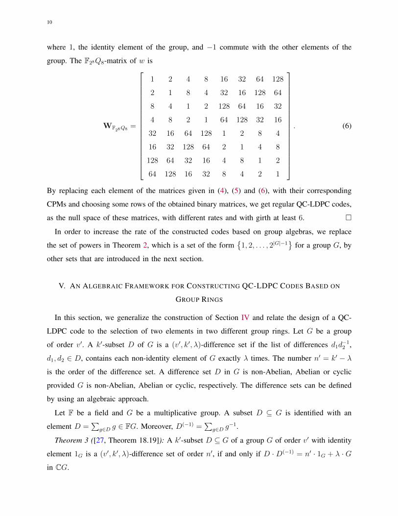

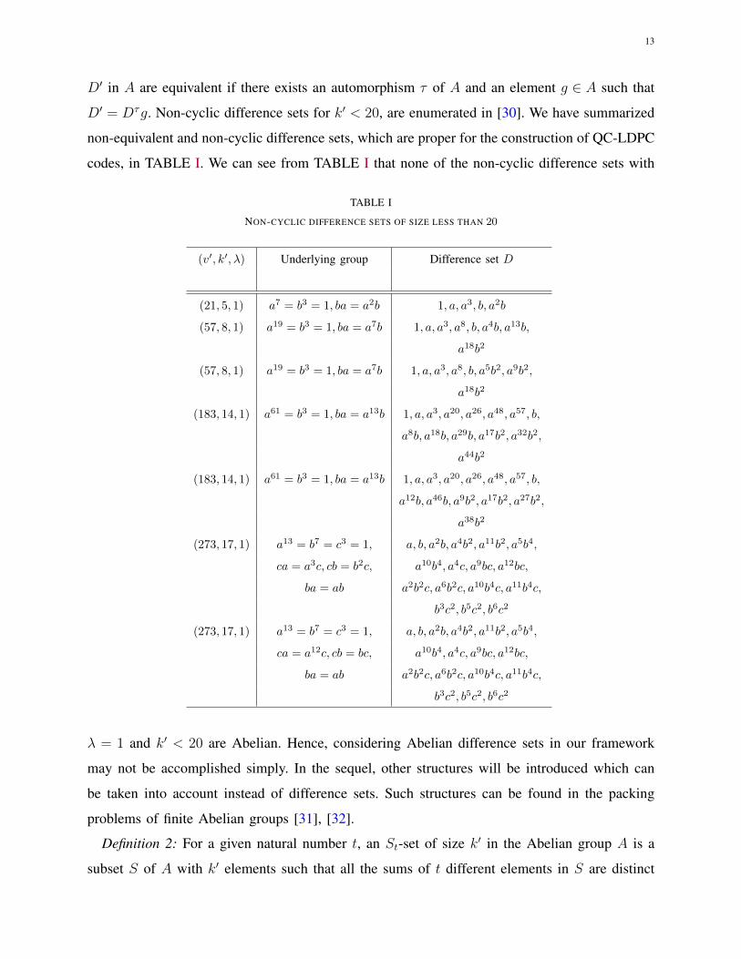


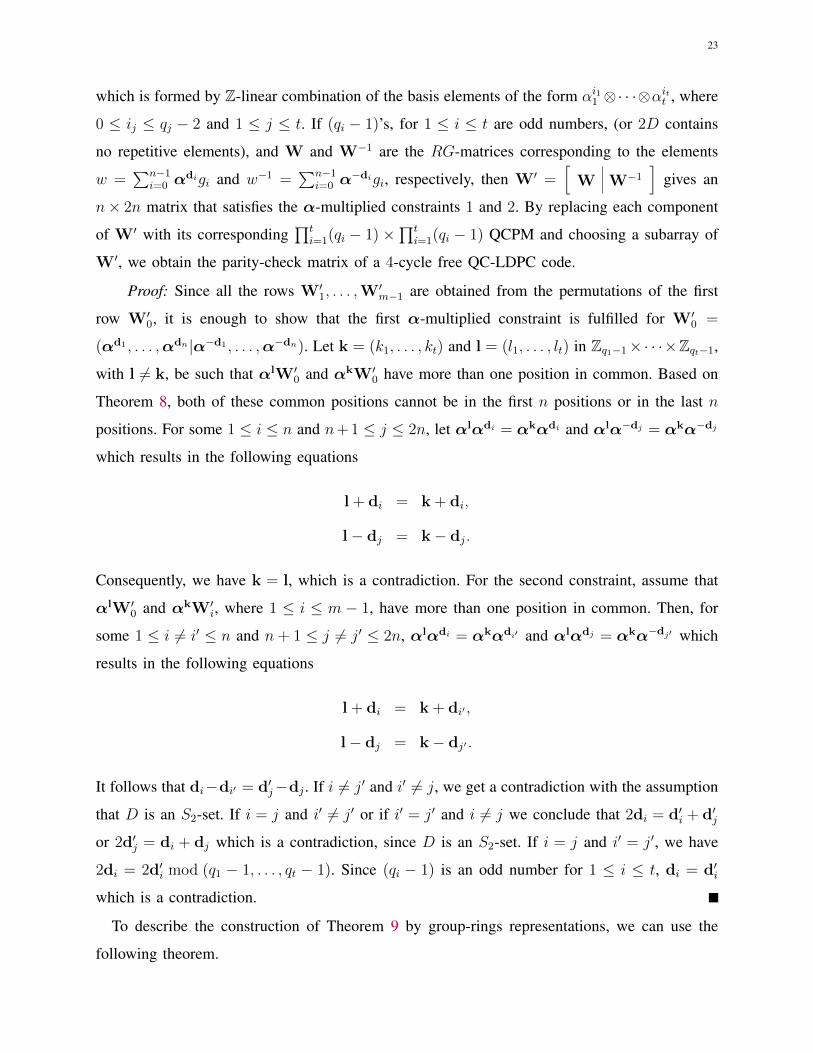


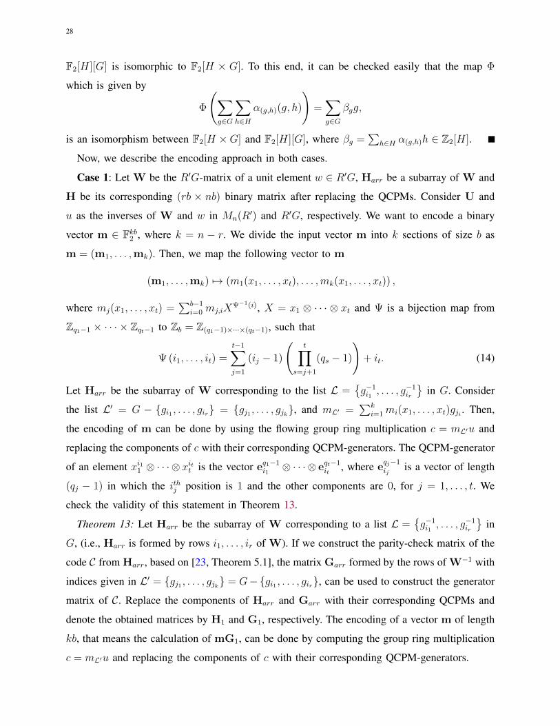
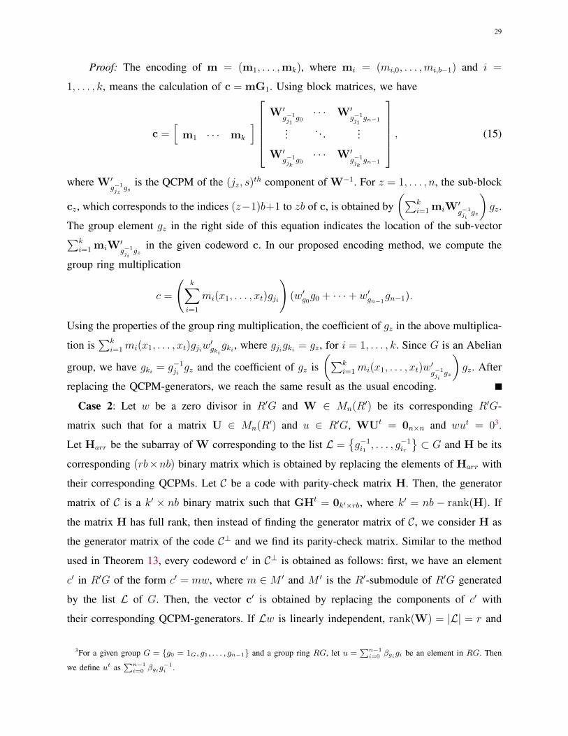

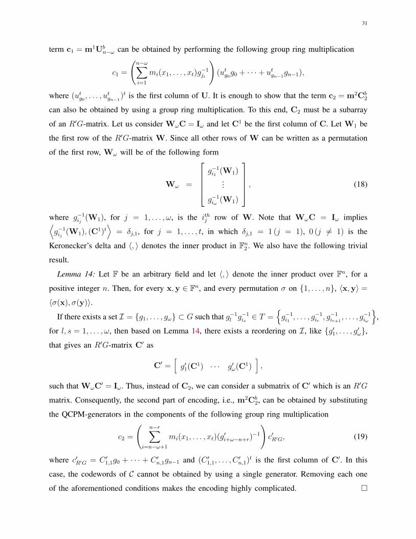


![CFMA (Compute-Forward Multiple Access) and its ... · error-correcting codes along with ecient encoding and decoding algorithms. In particular, Turbo codes [2], LDPC codes [3] and](https://static.documents.pub/doc/80x56/5eb72dbe7b8e3c02ed2c5aaa/cfma-compute-forward-multiple-access-and-its-error-correcting-codes-along.jpg)


![Design LDPC Cycle - Utah ECEPeng/Itw07.pdfoptimized binary LDPC code in [5] by 0.38 dB. Due to its highly irregular degree sequence, the encoding complexity of the optimized binary](https://static.documents.pub/doc/80x56/5ec0dbf12cbe9516c23239ee/design-ldpc-cycle-utah-pengitw07pdf-optimized-binary-ldpc-code-in-5-by-038.jpg)


