Continuous dynamic monitoring of an offshore wind turbine on a monopile foundation

C. Devriendt1, M. El Kafafy1, G. De Sitter1 , P.J. Jordaens2, P. Guillaume1 1 Vrije Universiteit Brussel, Acoustic and Vibration Research Group, Pleinlaan 2 B, B-1050, Elsene, Belgium e-mail: cdevrien@vub.ac.be 2 Sirris Celestijnenlaan 300 C, B-3001, Heverlee, Belgium

Abstract In order to minimize O&M costs and to extend the lifetime of offshore wind turbines it will be of high interest to continuously monitor the vibration levels and the evolution of the frequencies and damping ratios of the first modes of the foundation structure. This will allow us to identify and avoid resonant behavior and will also be able to give indications about the current state of the offshore wind turbine. State-of-the-art operational modal analysis techniques can provide accurate estimates of natural frequencies, damping ratios and mode shapes. To allow a proper continuous monitoring during operations a fast and reliable solution, which is applicable on industrial scale, needs to be developed. The methods need also to be automated and their reliability improved, so that no human-interaction is required and the system can track changes in the dynamic behavior of the offshore wind turbine. This paper will present and discuss the approach that will be used for the long-term monitoring campaign on an offshore wind turbine in the Belgian North Sea.

1 Introduction

1.1 Relevance

Online monitoring of wind turbines is a more and more critical issue as the machines are growing in size and offshore installations are becoming more common. To increase the power generation and limit the weight, the turbines are becoming structurally more flexible, thus an accurate prediction of their dynamic behavior is mandatory. On the other hand, inspection and maintenance for offshore installations are much more cumbersome and expensive than for onshore turbines. Thus a remote monitoring application with the ability to predict structural changes can help to reduce catastrophic failures and their associated costs.

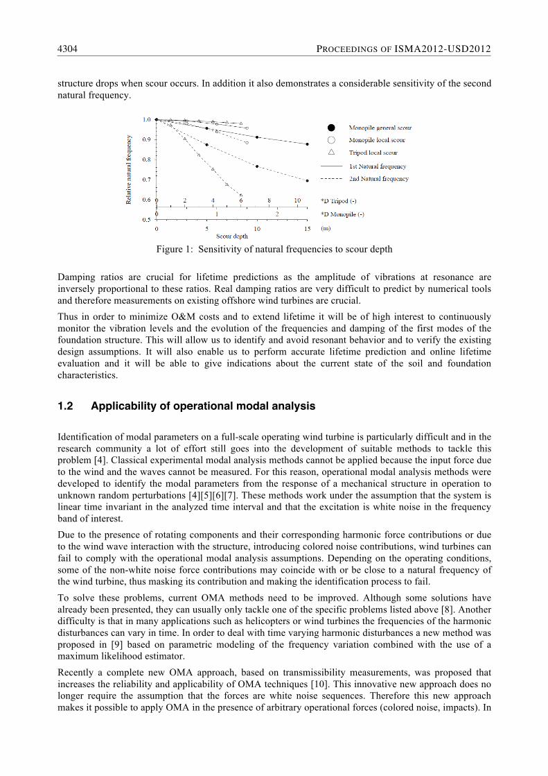
When it comes to foundation, scouring and reduction in foundation integrity over time are especially problematic because they reduce the fundamental structural resonance of the support structure, aligning that resonance more closely to the lower frequencies at which much of the broadband wave and gust energy is contained or because they align this resonance more closely with 1P. Thus the lower the natural frequency means that more wave energy can create resonant behavior increasing fatigue damage [1]. Currently it is not possible to forecast the extent of scour that forms around the foundation due to currents at the sea bed. The investigation of scour-monitoring methods require field measurements of scour depths around the monopile. Numerical analysis [2] shows that the natural frequency is notably affected by scour. In [3] a study of the dynamic behavior for a tripod and monopile design of a 6 MW turbine is presented. The results of this study are shown in figure 1. It is shown that the natural frequency of the support

4303

structure drops when scour occurs. In addition it also demonstrates a considerable sensitivity of the second natural frequency.

Figure 1: Sensitivity of natural frequencies to scour depth

Damping ratios are crucial for lifetime predictions as the amplitude of vibrations at resonance are inversely proportional to these ratios. Real damping ratios are very difficult to predict by numerical tools and therefore measurements on existing offshore wind turbines are crucial. Thus in order to minimize O&M costs and to extend lifetime it will be of high interest to continuously monitor the vibration levels and the evolution of the frequencies and damping of the first modes of the foundation structure. This will allow us to identify and avoid resonant behavior and to verify the existing design assumptions. It will also enable us to perform accurate lifetime prediction and online lifetime evaluation and it will be able to give indications about the current state of the soil and foundation characteristics.

1.2 Applicability of operational modal analysis

Identification of modal parameters on a full-scale operating wind turbine is particularly difficult and in the research community a lot of effort still goes into the development of suitable methods to tackle this problem [4]. Classical experimental modal analysis methods cannot be applied because the input force due to the wind and the waves cannot be measured. For this reason, operational modal analysis methods were developed to identify the modal parameters from the response of a mechanical structure in operation to unknown random perturbations [4][5][6][7]. These methods work under the assumption that the system is linear time invariant in the analyzed time interval and that the excitation is white noise in the frequency band of interest. Due to the presence of rotating components and their corresponding harmonic force contributions or due to the wind wave interaction with the structure, introducing colored noise contributions, wind turbines can fail to comply with the operational modal analysis assumptions. Depending on the operating conditions, some of the non-white noise force contributions may coincide with or be close to a natural frequency of the wind turbine, thus masking its contribution and making the identification process to fail.

To solve these problems, current OMA methods need to be improved. Although some solutions have already been presented, they can usually only tackle one of the specific problems listed above [8]. Another difficulty is that in many applications such as helicopters or wind turbines the frequencies of the harmonic disturbances can vary in time. In order to deal with time varying harmonic disturbances a new method was proposed in [9] based on parametric modeling of the frequency variation combined with the use of a maximum likelihood estimator.

Recently a complete new OMA approach, based on transmissibility measurements, was proposed that increases the reliability and applicability of OMA techniques [10]. This innovative new approach does no longer require the assumption that the forces are white noise sequences. Therefore this new approach makes it possible to apply OMA in the presence of arbitrary operational forces (colored noise, impacts). In

4304 PROCEEDINGS OF ISMA2012-USD2012

recent work it was shown that the transmissibility based OMA approach is able to deal successfully with harmonics when the loads are correlated [11]. The proposed transmissibility based OMA approach therefore looks very appealing. However, despite the good results obtained so far there is a need for more basic research in order to continue to refine this approach and correctly position it in relation to other OMA methods.

In [12] the violation of the time invariance assumption in the case of operational wind turbines was discussed. During operation a wind turbine is subjected to different motions of the substructures, e.g. yaw-motion of the nacelle, the individual pitching of the blades and the overall rotation of the rotor.

Rotor rotation represents a severe problem from structure invariance point of view [13]. However if one is interested in the fundamental tower modes the effect of the rotor can be considered as an external excitation [12]. During operation the yaw motion does not present a considerable problem for modal analysis as the yaw speed is very slow and the nacelle does not move constantly. Therefore it is possible to select datasets when the yaw does not change at all. Pitch-controlled wind turbines are designed to operate at variable speed, thus the assumption of linear time invariant system may not be valid. This poses a serious problem in the selection of an adequate length of the time signal for the analysis [5]. While the duration should be long enough to allow a proper estimation of modal parameters and in particular of damping values, on the other hand it is necessary to use signals obtained for “quasi-stationary” conditions to comply with the invariant system assumption. Different regimes can be identified e.g. pitch-regulated regime; RPM-regulated regime and parked conditions. Obviously in parked conditions the system is time invariant and OMA assumptions are fulfilled. Also in the RPM-regulated regime OMA is possible as the pitch is set to minimum and does not change a lot in time.

Therefore we can conclude that, in order to achieve accurate OMA estimates, pre-processing, that includes automatic selection of the time signals with a sufficient duration and almost stationary operating conditions, needs to be implemented.

2 Offshore measurements

2.1 Description of measurement setup

The measurement campaigns are performed at the Belwind wind farm, which consists of 55 Vestas V90 3MW wind turbines. The wind farm is located in the North Sea on the Bligh Bank, 46 km off the Belgian coast (Figure 2).

Figure 2: location Belwind wind farm (1) park layout (2) measurement locations (3)

The hub-height of the wind turbine is on average 72m above sea-level. Each transition piece is 25m heigh and has a weight of 120 ton. The tests are performed on the BBCO1-turbine that is located in the north of the wind farm directly next to the offshore high voltage substation (OHVS).

The wind turbine is placed on a monopile foundation structure with a diameter of 5m and a wall-thickness of 7cm. The actual water depth at the location of BBCO1 is 22.9m and the monopile has a penetration depth of 20.6m. The soil is considered stiff and mainly consists of sand.

WIND TURBINE VIBRATIONS 4305

The structures instrumented in this campaign are the tower and transition piece. Measurements are taken at 4 levels on 9 locations using a total of 10 sensors. The measurement locations are indicated in Figure 2 by yellow circles. The locations are chosen based on the convenience of sensor mounting, such as the vicinity of platforms. The chosen levels are 67m, 37m, 23m and 15m above sea level. The interface level between the transition piece and the wind turbine is at 17m above sea level. There are two accelerometers mounted at the lower three levels and four at the top level. The chosen configuration is primarily aimed at identification of tower bending modes. The two extra sensors on the top level are placed to capture the tower torsion. Accelerometers have been selected, which have a high sensitivity and are able to measure very low frequent signals. This is necessary considering that the modal frequencies of interest, for the wind turbine structure, are expected to be around 0.35Hz, and the expected vibration magnitude is very low, especially during ambient excitation.

The data-acquisition system is mounted in the transition piece (green circle in Figure 2). A Compact Rio system of National Instruments was used (Figure 3). An important reason for choosing this particular type of system is its high flexibility to measure different types of signals, e.g. accelerations and strains. Since the project aims at characterizing the dynamics during a long period, it was also required that the data-acquisition system can be remotely accessed and is capable of automatic startup in case of power shutdowns.

Figure 3: Data acquisition system based on NI Compact Rio System (left) and logger software (right)

The data acquisition software allows for the continuous monitoring of the accelerations. The software measures continuously and sends data every 10 minutes to the server that is installed onshore using a dedicated fiber that is running over the sea-bed. All data receives a time-stamp from a NTP timeserver in order to be able to correlate them with the SCADA and Meteo data. The measurements can be monitored real-time using the online scope-function. In order to classify the operating conditions of the wind turbine during the measurements SCADA data (power, rotor speed, pitch angel, nacelle direction) is gathered at a sample rate of 1Hz. To also monitor the varying environmental conditions, the ambient data (wind speed, wind direction, significant wave height, air temperature, ...) is being collected at 10 minute intervals.

The data-acquisition system was programmed to acquire data with a sampling ratio of 5kHz. Considering the frequency band of interest and in order to reduce the amount of data the recorded time series have been filtered with a band-pass filter and re-sampled with a sampling frequency of 12.5Hz. After the downsampling and filtering a coordinate transformation was performed. The accelerometers are mounted on the tower. Therefore, in order to measure the vibrations along the axis of the nacelle, it is necessary to take the yaw-angle into account by transforming them into the coordinate system of the nacelle [13].

2.2 Overspeed Stop

To have a first estimate for the fundamental modes of the tower and foundation an overspeed test was performed to have a free-decay measurement with signals of high acceleration levels.

For the overspeed stop the wind speed was the minimum required 6.5m/s. During an overspeed stop the wind turbine speeds up until it reaches 19.8 rpm. Then the wind turbine is automatically shut down. During this stop the pitch angle is changed from -2.5 to 88.2 degrees in a couple of seconds. The thrust release due to this sudden collective pitch variation excites the tower mainly in the wind direction as can be seen in Figure 4. Note that on the figure the wind direction is shown from left to right. Figure 4 also shows an example of the measured accelerations during the overspeed test on the different levels.

4306 PROCEEDINGS OF ISMA2012-USD2012

The objective was also to obtain an estimate of only the additional offshore damping. This is the overall damping excluding the aerodynamic damping and damping due to vortex shedding or installed damping devices [24]. Therefore during the overspeed test the tuned mass damper was turned off. We can also assume that the aerodynamic damping can be neglected a few seconds after the overspeed stop took place. Thus the measured additional offshore damping will consist of damping from wave creation due to structure vibration, viscous damping due to hydrodynamic drag, material damping of steel and soil damping due to inner soil frictions [2].

Figure 4: Movement seen from above (left) Example measured accelerations during overspeed stop (right) The Fast Fourier Transformation of the decaying functions can directly be used as input for the analysis methods in the frequency domain. Figure 5 shows the Fast Fourier Transformation of the accelerations obtained on the 3 different levels in the direction of the nacelle. One can clearly identify the dominant peak from the first for-aft (FA) mode around 0.35Hz.

Figure 5: Fast Fourier transformation of the accelerations (left) Polymax stabilization diagram

The identification algorithm can now be applied to a matrix with a single column containing the Fast Fourier Transformation of the free decays measured during the overspeed test. During this analysis we used again the data between 0.9 and 0.2 of the maximum acceleration. An estimate was obtained with a least squares frequency domain estimator, using polynomials with orders between 1 and 32 [7]. The fitting was performed in the frequency range 0.1–2Hz. In the corresponding stabilization diagram (Figure 5) with increasing model orders one can clearly identify several stable poles. By manual selecting the stable poles we can obtain the frequencies, damping values and mode shapes of the identified modes (Table 1).

Frequency (Hz) Damping (%)

0.3529 1.0539 1.0550 0.4508 1.1870 0.6794 1.3562 0.9598 1.4799 1.5876 1.5405 0.7980

Table 1: Frequencies and damping of

modes identified with the overspeed test Figure 6: First and second FA mode shape

WIND TURBINE VIBRATIONS 4307

By analyzing the mode shapes the first FA and second FA mode could clearly be identified at respectively 0.35Hz and 1.19Hz. The mode shapes are shown in Figure 6. The frequency below the dominant mode was identified with a a frequency of 0.29Hz. This perfectly coincides with the wave period of the waves with a wave direction almost in line with the nacelle. During the overspeed stop the wave period was around 3.4 seconds. The other stable modes are due to the contributions of a torsion tower mode and blades modes in the overall vibration of the wind turbine during an overspeed stop.

3 Continuous Dynamic Monitoring

During the long term measurement campaign our aim is to continuously monitor the vibration levels and the evolution of the frequencies and damping values of the first 2 fundamental modes of the tower and foundation. Both the resonance frequencies and damping values are crucial to quantify the reliability and the lifetime of offshore wind turbines during its life-cycle. These parameters will also be analyzed to see if they can provide indications about the current state of the soil and foundation characteristics for e.g. monitoring scour development [3]. To allow a proper structural health monitoring during operations, based on e.g. the dynamic properties of the foundation and other wind turbine components, a fast and reliable solution which is applicable on industrial scale needs to be developed. The methods need also to be automated and their reliability improved, so that no human interaction is required and the system can track changes in the vibration pattern and distinguish between variation associated to varying operating conditions and those truly associated with a defect. Methods that allow estimating a confidence interval for the identified parameters should also be used.

In [15][16] automated modal identification approaches are presented based on the use of a frequency-domain maximum likelihood estimator (MLE) and stochastic validation criteria combined with a fuzzy C-means clustering approach, yielding promising results. In [17] the authors developed a methodology for automatic identification of modal parameters, using parametric identification methods, based on a hierarchical clustering algorithm. They successfully applied this technique for the continuous monitoring of a bridge. In this work the algorithm used to automate the identification process is a combination of above approaches and consists of the following 3 steps:

• Step 1: Identification of a model with high order using the p-LSCF estimator.

• Step 2: Perform a hierarchical clustering algorithm on the identified poles

• Step 3: Classification and evaluation of the identified clusters using a fuzzy clustering algorithm based on different validation criteria

These steps will be validated on data sets while the wind turbine was in parked conditions. This allows us to comply with the time-invariant OMA assumptions and avoid the presence of harmonic components.

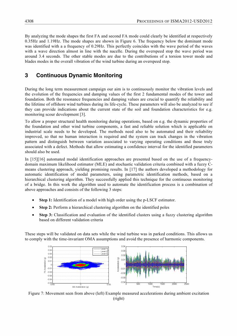
Figure 7: Movement seen from above (left) Example measured accelerations during ambient excitation

(right)

4308 PROCEEDINGS OF ISMA2012-USD2012

Also during the ambient excitation test the tuned mass damper was turned off. During the ambient excitation the wind speed was always very low <4.5m/s and the pitch angle was around 80.5 degrees. This permits us to assume that the aerodynamic damping can again be neglected. In figure 7 one can notice that the movement of the tower is still mainly in the direction of the nacelle and the wind, however a small side-to-side movement is also present. Figure 7 also shows an example of the accelerations measured by the different sensors during ambient excitation. When using the vibrations measured during the ambient vibrations one can calculate the correlation function of the measured accelerations. It has been shown that the output correlation of a dynamic system excited by white noise is proportional to its impulse response [18]. Therefore, the Fast Fourier Transformation of the positive time lags of the correlation functions can directly be used as input for the analysis methods in the frequency domain. The least squares estimators in the frequency domain can be applied to a matrix with the auto and cross correlation functions taking the two sensors on the top (c.f. Figure 2) in the FA and SS-direction as reference signals. The parameters that need to be chosen are the length of the used time segment and the number of time lags taken from the correlation function used for the spectra calculation [19]. The spectra resolution, controlled by the number of time lags taken from the correlation functions, should be high enough to well characterize all the modes within the selected frequency band. At the same time, it should be kept as low as possible to reduce the effect of the noise. Therefore, the algorithms in this paper will be tested for different time segment length, respectively for 40, 30, 20 and 10 minutes. For each time segment length, different numbers of time lags taken from the correlation functions are evaluated. This leads to different spectra resolutions. For each time segment, the different points taken from the correlation functions are 256, 512, 1024 and 2048 and 3075, which leads to a frequency resolution between 0.0488Hz and 0.0061Hz.

The objective of this comparison is mainly to check the quality of the results in order to evaluate if we would be able to use 10 minutes for the time segments used in the continuous monitoring of the offshore wind turbine. A time segment of 10 minutes allows to assume that the ambient condition e.g. wind speeds stayed more or less constant. 10 minutes is also the commonly used time interval for the SCADA data and the Meteo data, and thus has the advantage of making future analyses of the data easier.

3.1 Modal Parameter Identification

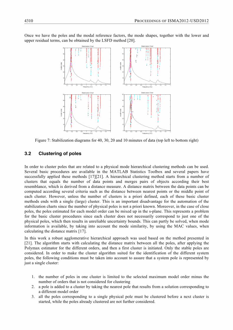
First the poles (and the modal participation factors) are estimated with the polyreference LSCF (also called PolyMAX algorithm) [20] for different model orders. These results can be used to construct a stabilization chart from which the user can try to separate the physical poles (corresponding to a mode of the system) from the mathematical ones. By displaying the poles (on the frequency axis) for an increasing model order (i.e number of modes in the model), the diagram helps to indicate the physical poles since, in general, they tend to stabilize for an increasing model order, while the computational poles scatter around. As a result, a construction of the stabilization chart is nowadays one of the requirements for a modal parameter estimation algorithm, and it has become a common tool in modal analysis. In figure 8 the stabilization diagrams are displayed for the different time-segments and a model order of maximum 60. In these cases 512 time lags were taken from the correlation functions. All stabilization diagrams seem to have around 5 or 6 well identifiable stable poles. In all cases the fundamental bending modes around 0.35Hz and 1.2Hz result in stable lines. Only in the case of 10 minutes the stabilization diagram becomes a bit less clear for higher orders around the first mode. We can manually select the poles in the stabilization diagram by clicking on the stable poles, indicated by a red s. It is clear that this may depend on the user. The results of such a manual selection are found in table 1. For high noise levels the stabilization diagrams can be difficult to interpret and give different results depending on the user. Moreover, stabilization diagrams require interaction and therefore they cannot directly be used when an autonomous modal parameter estimation is needed. In several papers it was noticed that the PolyMAX method produces very clear stabilization diagrams. This makes this method in particular interesting to try to automate the process.

WIND TURBINE VIBRATIONS 4309

Once we have the poles and the modal reference factors, the mode shapes, together with the lower and upper residual terms, can be obtained by the LSFD method [20].

 

 Figure 7: Stabilization diagrams for 40, 30, 20 and 10 minutes of data (top left to bottom right)

3.2 Clustering of poles

In order to cluster poles that are related to a physical mode hierarchical clustering methods can be used. Several basic procedures are available in the MATLAB Statistics Toolbox and several papers have successfully applied these methods [17][21]. A hierarchical clustering method starts from a number of clusters that equals the number of data points and merges pairs of objects according their best resemblance, which is derived from a distance measure. A distance matrix between the data points can be computed according several criteria such as the distance between nearest points or the middle point of each cluster. However, unless the number of clusters is a priori defined, each of these basic cluster methods ends with a single (large) cluster. This is an important disadvantage for the automation of the stabilization charts since the number of physical poles is not a priori known. Moreover, in the case of close poles, the poles estimated for each model order can be mixed up in the s-plane. This represents a problem for the basic cluster procedures since each cluster does not necessarily correspond to just one of the physical poles, which then results in unreliable uncertainty bounds. This can partly be solved, when mode information is available, by taking into account the mode similarity, by using the MAC values, when calculating the distance matrix [17].

In this work a robust agglomerative hierarchical approach was used based on the method presented in [21]. The algorithm starts with calculating the distance matrix between all the poles, after applying the Polymax estimator for the different orders, and then a first cluster is initiated. Only the stable poles are considered. In order to make the cluster algorithm suited for the identification of the different system poles, the following conditions must be taken into account to assure that a system pole is represented by just a single cluster:

1. the number of poles in one cluster is limited to the selected maximum model order minus the

number of orders that is not considered for clustering 2. a pole is added to a cluster by taking the nearest pole that results from a solution corresponding to

a different model order 3. all the poles corresponding to a single physical pole must be clustered before a next cluster is

started, while the poles already clustered are not further considered.

4310 PROCEEDINGS OF ISMA2012-USD2012

Each time a new cluster is initiated, a new distance matrix is computed using the remaining poles. When looking for a new pole to be added to a cluster an initially frequency interval (i.e. 1% of the mean frequency of the initiated cluster) is considered. In our case it was possible to consider such a small interval from the start because of the high quality of the measurements and the corresponding estimates. When the noise levels of the collected data is higher a larger interval can be used. A good rule when choosing the interval is to use the limit defined for the stabilization diagrams. As long as the number of poles, each corresponding to a different model order, is larger than the maximum number of poles that a cluster can contain, the width of the frequency interval is reduced. This maximum number of poles equals the maximum model order minus the number of orders that is not considered for clustering. One can choose not to use the first orders for the clustering algorithm, because the low order estimates can be of less quality and because the different system poles only show up as stable lines for higher model orders. One can also choose not to consider clusters with a small number of poles. Figure 8 shows the results of the algorithm when using 40, 30, 20 and 10 minutes of ambient data. The first 36 orders were not used and only clusters with more than 20% of the maximum number of poles a cluster can contain were retained.

 

 Figure 8: clusters obtained when using respectively 40, 30, 20 and 10 minutes of data (top left to bottom

middle) Zoom on clusters around first FA mode when using 10 minutes of data (bottom right) When using for example the data-set of 40 minutes 10 clusters were created. For the 10 minute case it was already observed in the stabilization diagram that the poles were more scattered around the main peak, making the manual pole-selection less obvious. When we look however to the results of the clustering-algorithm we can clearly see 3 clusters appearing and we can easily identify the cluster for the first for-aft mode (Figure 8). Therefore, this seems to be an efficient approach for the automatic identification. Based on the cluster results, a statistical analysis yields the mean and standard deviation for each of the estimated poles and hence for the damped natural frequencies and damping ratios. In table 2 the mean values are presented for comparison with the manual selection from the stabilization diagrams. The standard deviation on the frequencies and damping values can be used for validation purposes and the separation of physical and mathematical poles. One can also calculate an identification success-rate by dividing the number of poles in each cluster by the maximum number of poles a cluster can contain. These parameters will be used in the next paragraph to distinguish the well-identified clusters from the clusters with estimates of less quality or to distinguish the physical poles from the mathematical ones. Note that we did not include mode information in the cluster analysis. Other cluster algorithms include the MAC values between all the different poles when calculating the distance matrix [17]. In our research it was decided to base the clustering only on the poles, because useful mode-information might not always be available; this might especially be the case when only a small number of sensors is used. If mode information is available it will be used to distinguish physical from not physical poles as will be discussed later in this paper.

WIND TURBINE VIBRATIONS 4311

Table 2: Frequencies and damping values of identified modes by manual selection and by cluster analysis.

Figure 10 gives a visual overview of the mean values identified from the clusters when using the different time-segments. All time segments seem to be able to identify almost an equal number of clusters with similar mean frequencies. The scatter on damping is rather high, but for the 2 main modes of interest, respectively around 0.35Hz and 1.2Hz, the clusters have similar damping values. A zoom on the first 2 for-aft modes including the estimated standard deviation is shown in figure 10. Although the standard deviation when using only 10 minutes is higher than for the other data sets, especially for the first mode, the mean values are comparable and thus 10 minutes are considered sufficient to find estimates for the damping of the first foundation modes with acceptable quality.

 Figure 10: Overview mean values for damping and frequencies (left) for the first FA mode (middle) and

second FA mode (right) for 40 (red) 30 (green) 20 (blue) and 10 minutes (black)

The next figure shows the results for 10 minutes when a different number of time lags of the correlation functions is used, respectively 256, 1024 and 2048 points. It is known that taking a long correlation functions (e.g. taking 2048 points), especially with the short time data set, the noise effects increase and the information about the vibration modes decreases. When looking to the results of the cluster algorithm, both for 1024 points and 2048 points, a low number of clusters were identified. When we focus on the first mode we can observe that, when using 256 points and 2048 points, the standard deviations are high, and also the mean values are overestimated (Figure 13). Also, for the second mode these 2 cases result in a

4312 PROCEEDINGS OF ISMA2012-USD2012

slightly higher standard deviation and again in the case of 2048 points the damping value is very different (Figure 13). When using 1024 points the standard deviations are very low, but for the second mode the mean value seems to be underestimated. In the case of 512 time lags a high number of clusters were identified and we found mean values for the frequency and damping with acceptable standard deviations. To sum up, these analyses show that concerning the number of time lags taken from the correlation functions, 512 time lags seem to be adequate.

 

Figure 12: clusters obtained when using 10 minutes of data for 256, 1024 and 2048 time lags taken from the correlation functions

 

 

Figure 13: Mean values for damping and frequencies and standard deviation on damping for the first FA mode (left) and second FA mode (right) when using 10 minutes of data for respectively 256 (red), 512

(green), 1024 (blue) and 2048 (black) time lags Finally, a cluster analysis was done on 3 more successive data sets of 10 minutes and using 512 time lags of the correlation functions. All data sets resulted in clear identifiable clusters (Figure 14). Figure 15 gives the mean values for damping values and frequencies and standard deviation on damping values for the first FA mode and second FA mode. From these figures we can already see the variations on the estimates one might expect when using successive data-sets with similar ambient and operating conditions. For the damping values we can notice a variation from around 0.8% to 1.1% for both modes, i.e. a relative change of around 30%. The change in frequency is around 0.05Hz for the second mode and smaller than 0.02Hz for the first mode, i.e. a relative change of around 5%.

     

Figure 14: clusters obtained when using 3 successive data sets of 10 minutes and using 512 time lags  

 

WIND TURBINE VIBRATIONS 4313

   Figure 15: Mean values for damping and frequencies and standard deviation on damping for the first FA

mode (left) and second FA mode (right) for 4 successive 10 minute data-sets (red-green-blue-black)

Note that in [22] it was mentioned that in case of noisy data the damping values obtained by the p-LSCF method might be underestimated. It was also shown that in these cases the quality can be further improved by the poly-reference maximum-likelihood frequency domain (p-MLFD) algorithm. The starting values needed by the p-MLFD are provided by the p-LSCF algorithm.

3.3 Classification of clusters

The clustering procedure assures that each of the system poles will be represented by just one single cluster. However, since typically high model orders are chosen for reasons of noise on the data as well as the use of a discrete time transfer function model, not each cluster corresponds to a system pole. Therefore, each of the clusters needs to be assessed for its physicalness. Secondly, when continuous monitoring is done not all data-sets will allow to identify the physical modes and their corresponding frequencies and damping values with high confidence. Therefore criteria can be defined that can distinguish physical modes from mathematical ones and that allow to discard estimates of low quality.

In the case of the p-LSCF with varying model order and the proposed hierarchically clustering approach, the number of poles in a cluster, or the identification success rate, as well as the standard deviations on the frequencies and damping values of each cluster, may give a good indication for the physicalness and quality of the identified poles and their clusters. When a sufficient number of sensors is available mode shape information can be used to further evaluate the clusters by also considering the well-known validation criteria such as the Modal Assurance Criteria, Modal Phase Collinearity (MPC) and the Modal Phase Deviation (MPD). For each pole in a cluster the corresponding mode shape information can be computed and the following percentage ratios can e.g. be calculated: the fraction of mode shapes that have a Modal Phase Collinearity (MPC) larger than 80% and a Modal Phase Deviation (MPD) smaller than 10 degrees. An iterative Fuzzy C-means clustering algorithm, proven to be useful for the automation of the modal mode extraction, can now be used to evaluate the clusters. In [15][16] the approach was used to classify the identified poles into physical and computational poles. Based on the results for each of the validation criteria, the clusters identified after the first step can now also be grouped into two classes using this algorithm, i.e. clusters with physical and computational poles. The algorithm is implemented in the MATLAB Fuzzy Logic Toolbox. Following validation criteria will be used: Variable 1: the standard deviations of the estimated resonance frequencies Variable 2: the standard deviations of the estimated damping values Variable 3: the identification success rate Variable 4: fraction of mode shapes that have a Modal Phase Collinearity (MPC) larger than 80% Variable 5: the fraction of mode shapes with a Modal Phase Deviation (MPD) smaller than 10 degrees

4314 PROCEEDINGS OF ISMA2012-USD2012

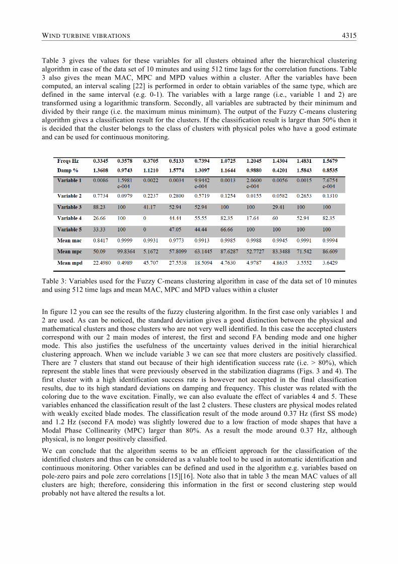
Table 3 gives the values for these variables for all clusters obtained after the hierarchical clustering algorithm in case of the data set of 10 minutes and using 512 time lags for the correlation functions. Table 3 also gives the mean MAC, MPC and MPD values within a cluster. After the variables have been computed, an interval scaling [22] is performed in order to obtain variables of the same type, which are defined in the same interval (e.g. 0-1). The variables with a large range (i.e., variable 1 and 2) are transformed using a logarithmic transform. Secondly, all variables are subtracted by their minimum and divided by their range (i.e. the maximum minus minimum). The output of the Fuzzy C-means clustering algorithm gives a classification result for the clusters. If the classification result is larger than 50% then it is decided that the cluster belongs to the class of clusters with physical poles who have a good estimate and can be used for continuous monitoring.

Table 3: Variables used for the Fuzzy C-means clustering algorithm in case of the data set of 10 minutes and using 512 time lags and mean MAC, MPC and MPD values within a cluster

In figure 12 you can see the results of the fuzzy clustering algorithm. In the first case only variables 1 and 2 are used. As can be noticed, the standard deviation gives a good distinction between the physical and mathematical clusters and those clusters who are not very well identified. In this case the accepted clusters correspond with our 2 main modes of interest, the first and second FA bending mode and one higher mode. This also justifies the usefulness of the uncertainty values derived in the initial hierarchical clustering approach. When we include variable 3 we can see that more clusters are positively classified. There are 7 clusters that stand out because of their high identification success rate (i.e. > 80%), which represent the stable lines that were previously observed in the stabilization diagrams (Figs. 3 and 4). The first cluster with a high identification success rate is however not accepted in the final classification results, due to its high standard deviations on damping and frequency. This cluster was related with the coloring due to the wave excitation. Finally, we can also evaluate the effect of variables 4 and 5. These variables enhanced the classification result of the last 2 clusters. These clusters are physical modes related with weakly excited blade modes. The classification result of the mode around 0.37 Hz (first SS mode) and 1.2 Hz (second FA mode) was slightly lowered due to a low fraction of mode shapes that have a Modal Phase Collinearity (MPC) larger than 80%. As a result the mode around 0.37 Hz, although physical, is no longer positively classified. We can conclude that the algorithm seems to be an efficient approach for the classification of the identified clusters and thus can be considered as a valuable tool to be used in automatic identification and continuous monitoring. Other variables can be defined and used in the algorithm e.g. variables based on pole-zero pairs and pole zero correlations [15][16]. Note also that in table 3 the mean MAC values of all clusters are high; therefore, considering this information in the first or second clustering step would probably not have altered the results a lot.

WIND TURBINE VIBRATIONS 4315

Figure 16: Variables used for the clustering algorithm in case of the data set of 10 minutes and using 512

time lags and the cluster classification results in case of using variables 1 and 2 (top left) variables 1, 2 and 3 (top right) and using all 5 variable (bottom)

4 Conclusions

This paper presents an automated continuous monitoring approach for identifying the frequencies and damping values of the fundamental modes of an offshore wind turbine. The results are very promising since the approach is capable of identifying the modes of interest even when short data-sets of 10 minutes are used. It is shown that, by using the p-LSCF-estimator for varying model orders combined with a hierarchical clustering algorithm, accurate estimates can be obtained of many modes of the wind turbine together with a confidence interval. Finally, validation criteria can be calculated that allow to separate physical mode estimates from mathematical ones and allow discarding estimates of low quality by using a fuzzy clustering approach. The method can be successfully applied even without the need for extensive spatial information, which is important for the implementation of many monitoring systems.

Acknowledgements

The research presented in this paper is conducted in the framework of the “Offshore Wind Infrastructure Application Lab” (www.owi-lab.be).The authors gratefully thank the people of Belwind NV and NorthWind NV for their support before, during and after the installation of the measurement equipment. They also supplied all relevant operational and structural data which has been used for the analysis.

4316 PROCEEDINGS OF ISMA2012-USD2012

References

[1] Dwight Davis. Dr. Martin Pollack. Brian Petersen, “Evaluate the Effect of Turbine Period of Vibration Requirements on. Structural Design Parameters, Technical report of findings”, 2010.

[2] Van Der Tempel, “Design of Support Structures for Offshore Wind Turbines”, PhD T.U. Delft, 2006

[3] Zaaijer, M.B., Tripod support structure - pre-design and natural frequency assessment for the 6 MW DOWEC, Doc. no. 63, TUD, Delft, 14 May 2002.

[4] T.G. Carne and G.H. James III, The inception of OMA in the development of modal testing for wind turbines, Mechanical Systems and Signal Processing, 24, 1213-1226, 2010.

[5] L. Hermans, H. Vav Der Auweraer, Modal testing and analysis of structures under operational conditions: industrial applications, Mechanical Systems and Signal Processing, 13(2), 193216, 1999.

[6] R. Brincker, L. Zhang, and P. Andersen, Modal identification of output only systems using frequency domain decomposition, Smart Materials and Structures 10 (2001) pp. 441445, 2001.

[7] B. Cauberghe, Applied frequency-domain system identification in the field of experimental and operational modal analysis. PhD thesis, Vrije Universiteit Brussel, Belgium, avrg.vub.ac.be, 2004.

[8] B. Peeters, B. Cornelis, K. Jansenns, H. Van der Auweraer, Removing disturbing harmonics in Operational Modal Analysis, Proceedings of IOMAC 2007, Copenhagen, Denmark, 2007.

[9] R. Pintelon, B. Peeters and P. Guillaume, Continuous-time operational modal analysis in presence of harmonic disturbances, Mechanical Systems and Signal Processing, 22, 1017-1035, 2008.

[10] Devriendt C; Guillaume P, Identification of modal parameters from transmissibility measurements, Journal of Sound and Vibration, 314 (1- 2): 343-356 2008

[11] Devriendt C; De Sitter G; Vanlanduit S; Guillaume P; Operational modal analysis in the presence of harmonic excitations by the use of transmissibility measurements, MSSP, 23 (3):621-635 2009

[12] D. Tcherniak, S. Chauhan and M.H. Hansen, Applicability limits of Operational Modal Analysis to operational wind turbines, Proceedings of the IMAC XXVIII, Jacksonville, USA, 2010.

[13] S. Chauhan, D. Tcherniak, Jon Basurko, Oscar Salgado, Iker Urresti, Carlo E. Carcangiu and Michele Rossetti. Operational Modal Analysis of Operating Wind Turbines: Application to Measured Data, Volume 5, Proceedings of the Society for Experimental Mechanics Series, 2011, Vol. 8, 65-81

[14] N.J. Tarp-Johansen: „Comparing sources of damping of cross-wind motion”, EOW 2009 [15] S.Vanlanduit, P.Verboven, P.Guillaume, J.Schoukens, Anautomatic frequency domain modal

parameter estimation algorithm. J.SoundVib.265(3) (2003) 647–661.

[16] P.Verboven, E.Parloo, P.Guillaume , M.Van Overmeire, Autonomous structural health monitoring.Part1: modal parameter estimation and tracking , MSSP, 16(4)(2002)637–657.

[17] F.Magalhaes,A´Cunha,E.Caetano,On line automatic identification of the modal parameters of a long span arch bridge , Mech. Syst. Signal Process. 23 (2) (2009) 316–329.

[18] Filipe Magalhães, Álvaro Cunha, Elsa Caetano, Rune Brincker Damping estimation using free decays and ambient vibration tests, MSSP, Volume 24, Issue 5, July 2010, Pages 1274-1290

[19] Bendat, J.; Piersol, A. (1980) Engineering Applications of Correlation and Spectral Analysis.

[20] P. Guillaume, Peter Verboven, S. Vanlanduit, H. Van der Auweraer, B. Peeters, A poly-reference implementation of the least-squares complex frequency domain-estimator, IMAC 21, February 2003

[21] P.Verboven, B. Cauberghe, E. Parloo, S. Vanlanduit, P. Guillaume, User-assisting tools for a fast frequency-domain modal parameter estimation method, Mech.Syst.SignalProcess.18 (2004) 759–780

[22] B. Cauberghe, P. Guillaume, P. Verboven, E. Parloo, S. Vanlanduit, A poly-reference implementation of the maximum likelihood complex frequency-domain estimator and some industrial applications, in: Proceedings of the IMAC22, Dearborn (US), January 2004.

WIND TURBINE VIBRATIONS 4317

4318 PROCEEDINGS OF ISMA2012-USD2012