Continuous time Markov chains - Penn Engineeringese303/block_3_continuous_time... · Systems...

Continuous time Markov chains

Alejandro RibeiroDept. of Electrical and Systems Engineering

University of [email protected]

http://www.seas.upenn.edu/users/~aribeiro/

October 16, 2017

Stoch. Systems Analysis Continuous time Markov chains 1

mailto:[email protected]

http://www.seas.upenn.edu/users/~aribeiro/

Exponential random variables


Counting processes and definition of Poisson processes

Properties of Poisson processes


Transition probability function

Determination of transition probability function

Limit probabilities


Exponential distribution

I Exponential RVs are used to model times at which events occur

I Or in general time elapsed between occurrence of random events

I RV T ∼ exp(λ) is exponential with parameter λ if its pdf is

fT (t) = λe−λt , for all t ≥ 0

I The cdf, integral of the pdf, is (t ≥ 0) ⇒ FT (t) = 1− e−λt

I Complementary (c)cdf is ⇒ P(T ≥ t) = 1− FT (t) = e−λt

pdf cdf

0 0.5 1 1.5 2 2.5 3 3.5 4 4.50

0.2

0.4

0.6

0.8

1

0 0.5 1 1.5 2 2.5 3 3.5 4 4.50

0.2

0.4

0.6

0.8

1


Expected value

I The expected value of time T ∼ exp(λ) is

E [T ] =

∫ ∞0

tλe−λt = −te−λt∣∣∣∣∞0

+

∫ ∞0

e−λt = 0 +1

λ

I Integrated by parts with u = t, dv = λe−λt

I Mean time is inverse of parameter λ

⇒ λ is rate/frequency of events happening at intervals T

I Average of λt events in time t

I Bigger lambda, smaller expected times, larger frequency of events

∣∣S1

T1 ∣∣S2

T2 ∣∣S3

T3 ∣∣S4

T4 ∣∣S5

T5 ∣∣S6

T6 ∣∣S7

T7 ∣∣S8

T8 ∣∣S9

T9 ∣∣S10

T10

t∣∣∣∣∣t = 0

∣∣∣∣∣t = 5/λ

∣∣∣∣∣t = 10/λ


Second moment and variance

I For second moment also integrate by parts (u = t2, dv = λe−λt)

E[T 2]

=

∫ ∞0

t2λe−λt = −t2e−λt∣∣∣∣∞0

+

∫ ∞0

2te−λt

I Fisrt term is 0, second is, except for a constant, as computed before

E[T 2]

=2

λ

∫ ∞0

tλe−λt =2

λ2

I The variance is computed from the mean and variance

var [T ] = E[T 2]− E [T ]2 =

2

λ2− 1

λ2=

1

λ2

I Parameter λ controls mean and variance of exponential RV


Memoryless random times

I Consider random time T . We say time T is memoryless if

P[T > s + t

∣∣T > t]

= P [T > s]

I Probability of waiting s extra units of time given that we waited tseconds is just the probability of waiting s seconds

⇒ System does not remember it has already waited t units

⇒ Same probability irrespectively of time already elapsed

Ex: Chemical reaction A + B → AB occurs when molecules A and B“collide”. A, B move around randomly. Time T until reaction

Ex: Group of molecules of type A and type B. Reaction occurs whenany type A encounters any type B. Time T until next reaction


Exponential RVs are memoryless

I Write memoryless property in terms of joint pdf

P[T > s + t

∣∣T > t]

=P [T > s + t,T > t]

P [T > t]= P [T > s]

I Notice that having T > s + t and T > t is equivalent to T > s + t

I Replace P [T > s + t,T > t] = P [T > s + t] and reorder terms

P [T > s + t] = P [T > t]P [T > s]

I If T is exponentially distributed ccdf is P [T > t] = e−λt . Then

P [T > s + t] = e−λ(s+t) = e−λte−λs = P [T > t] P [T > s]

I If random time T is exponential ⇒ T is memoryless


Continuous memoryless RVs are exponential

I Consider a function g(t) with the property g(t + s) = g(t)g(s)

I Functional form of g(t)? Take logarithms

log g(t + s) = log g(t) + log g(s)

I Can only be true for all t and s if log g(t) = ct for some constant c

I Which in turn, can only true if g(t) = ect for some constant c

I Compare observation with statement of memoryless property

P [T > s + t] = P [T > t] P [T > s]

I It must be P [T > t] = ect for some constant c

I If T is continuous this can only be true for exponential T

I If T discrete it is geometric P [T > t] = (1− p)t with (1− p) = ec

I If continuous random time T is memoryless ⇒ T is exponential


Combining results

TheoremA continuous random variable T is memoryless if and only if it isexponentially distributed. That is

P[T > s + t

∣∣T > t]

= P [T > s]

if and only if fT (t) = λe−λt for some λ > 0

I Exponential RVs are memoryless. Do not remember elapsed time

I They are the only type of continuous memoryless RV

I Discrete RV T is memoryless if and only of it is geometric

I Geometrics are discrete approximations of exponentials

I Exponentials are continuous limits of geometrics

I Exponential = time until success ⇔ Geometric = nr. trials until success


Time to first event

I Independent exponential RVs T1, T2 with parameters λ1, λ2I Probability distribution of first event, i.e., T := min(T1,T2)?

I For having T > t we need both T1 > t and T2 > t

I Using independence of X and Y we can write

P [T > t] = P [T1 > t] P [T2 > t] =(1− FT1(t)

)(1− FT2(t)

)I Substituting expressions of exponential cdfs

P [T > t] = e−λ1te−λ2t = e−(λ1+λ2)t

I T is exponentially distributed with parameter λ1 + λ2

I Minimum of exponential variables is exponential

I Given two events happening at random exponential times (T1, T2)

⇒ Time to any of them happening is also exponential


First event to happen

I Prob. P [T1 < T2] of T1 ∼ exp(λ1) happening before T2 ∼ exp(λ2)

I Condition on T2 = t and integrate over the pdf of T2

P [T1 < T2] =

∫ ∞0

P[T1 < t

∣∣T2 = t]fT2(t) dt =

∫ ∞0

FT1(t)fT2(t) dt

I Substitute expressions for exponential pdf and cdf

P [T1 < T2] =

∫ ∞0

(1− e−λ1t)λ2e−λ2t dt =

λ1λ1 + λ2

I Either X comes before Y or vice versa then

P [T2 < T1] = 1− P [T1 < T2] =λ2

λ1 + λ2

I Probabilities are relative values of parameters

I Larger parameter ⇒ smaller average ⇒ larger prob. happening first


Probability of event in infinitesimal time

I Probability of an event happening in infinitesimal time h?

I Want P [T < h] for small h,

P [T < h] =

∫ h

0

λe−λt dt ≈ λh

I Equivalent to∂P [T < t]

∂t

∣∣∣∣t=0

= λ

I Sometimes also write P [T < h] = λh + o(h)

I o(h) implies limh→0

o(h)

h= 0 . Read as “negligible with respect to h”

I Two independent events in infinitesimal time h?

P [T1 ≤ h,T2 ≤ h] ≈ (λ1h)(λ2h) = λ1λ2h2 = o(h)


Counting and Poisson processes







Limit probabilities


Counting processes

I Stochastic process N(t) taking integer values 0, 1, . . . , i , . . .

I Counting process N(t) counts number of events occurred by time t

I Nonnegative integer valued: N(0) = 0, N(t) = 0, 1, 2, . . .,

I Nondecreasing: for s < t it holds N(s) ≤ N(t)

I Event counter: N(t)− N(s) = number of events in interval (s, t]I Continuous on the right

Ex.1: # text messages (SMS) typedsince beginning of class

Ex.2: # economic crisis since 1900

Ex.3: # customers at Wawa since8am this morning t

n(t)

123456

S1 S2 S3 S4 S5 S6


Independent increments

I Number of events in disjoint time intervals are independent

I Consider times s1 < t1 < s2 < t2 and intervals (s1, t1] and (s2, t2]

I N(t1)− N(s1) events occur in (s1, t1]. N(t2)− N(s2) in (s2, t2]

I Independent increments implies latter two are independent

P [N(t1)− N(s1) = k ,N(t2)− N(s2) = l ]

= P [N(t1)− N(s1) = k] P [N(t2)− N(s2) = l ]

Ex.1: Likely true for SMS, except for “have to send” messages

Ex.2: Most likely not true for economic crisis (business cycle)

Ex.3: Likely true for Wawa, except for unforeseen events (storms)

I Does not mean N(t) independent of N(s)

I These events are clearly not independent, since N(t) is at least N(s)


Stationary increments

I Prob. dist. of number of events depends on length of interval only

I Consider time intervals (0, t] and (s, s + t]

I N(t) events occur in (0, t]. N(s + t)− N(s) events in (s, s + t]

I Stationary increments implies latter two have same prob. dist.

P [N(s + t)− N(s) = k] = P [N(t) = k]

Ex.1: Likely true if lecture is good and you keep interest in the class

Ex.2: Maybe true if you do not believe we are becoming better atpreventing economic crisis

Ex.3: Most likely not true because of, e.g., rush hours and slow days


Poisson process

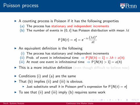
I A counting process is Poisson if it has the following properties

(a) The process has stationary and independent increments(b) The number of events in (0, t] has Poisson distribution with mean λt

P [N(t) = n] = e−λt(λt)n

n!

I An equivalent definition is the following

(i) The process has stationary and independent increments(ii) Prob. of event in infinitesimal time ⇒ P [N(h) = 1] = λh + o(h)(iii) At most one event in infinitesimal time ⇒ P [N(h) > 1] = o(h)

I This is a more intuitive definition (even though difficult to believe now)

I Conditions (i) and (a) are the same

I That (b) implies (ii) and (iii) is obvious.I Just substitute small h in Poisson pmf’s expression for P [N(t) = n]

I To see that (ii) and (iii) imply (b) requires some work


Explanation of model (i)-(iii)

I Consider time T and divide interval (0,T ] in n subintervals

I Subintervals are of duration h = T/n, h vanishes as n increases

I The m − th subinterval spans((m − 1)h,mh

]I Define Am as the number of events that occur in m − th subinterval

Am = N(mh)− N

((m − 1)h

)I The total number of events in (0,T] is the sum of Ams

N(T ) =n∑

m=1

Am=n∑

m=1

N(mh)− N

((m − 1)h

)I In figure, N(T ) = 5, A1, A2, A4, A7, A8 are 1 and A3, A5, A6 are 0

← h→ ← h→ ← h→ ← h→ ← h→ ← h→ ← h→ ← h→↓T1 ↓T2 ↓T3 ↓T4 ↓T5

t

∣∣∣∣t = 0

∣∣∣∣t = T


Probability distribution of Am (intuitive arg.)

I Note first that since increments are stationary as per (i), it holds

P [Am = k] = P[N(mh)− N

((m − 1)h

)= k

]= P [N(h) = k]

I In particular, using (ii) and (iii)

P [Am = 1] = P [N(h) = 1] = λh + o(h)

P [Am > 1] = P [N(h) > 1] = o(h)

I Set aside o(h) probabilities – They’re negligible with respect to λh

P [Am = 1] = λh P [Am = 0] = 1− λh

I Am is Bernoulli with parameter λh

← h→ ← h→ ← h→ ← h→ ← h→ ← h→ ← h→ ← h→↓T1 ↓T2 ↓T3 ↓T4 ↓T5

t

∣∣∣∣t = 0

∣∣∣∣t = T


Probability distribution of N(T ) (intuitive arg.)

I Since increments are also independent as per (i), Am are independent

I N(T ) is sum of n independent Bernoulli RVs with parameter λh

I N(T ) is binomial with parameters (n, λh) = (n, λT/n)

I As interval length h→ 0, number of intervals n→∞⇒ The product n(λh) = λT stays constant

I N(T ) is Poisson with parameter λT

I Then (ii)-(iii) imply (b) and definitions are equivalent

I Not a proof because we neglected o(h) terms. But explains what aPoisson process is

← h→ ← h→ ← h→ ← h→ ← h→ ← h→ ← h→ ← h→↓T1 ↓T2 ↓T3 ↓T4 ↓T5

t

∣∣∣∣t = 0

∣∣∣∣t = T


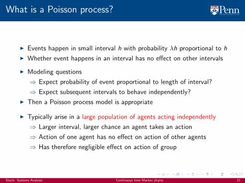
What is a Poisson process?

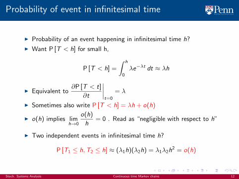
I Events happen in small interval h with probability λh proportional to h

I Whether event happens in an interval has no effect on other intervals

I Modeling questions

⇒ Expect probability of event proportional to length of interval?

⇒ Expect subsequent intervals to behave independently?

I Then a Poisson process model is appropriate

I Typically arise in a large population of agents acting independently

⇒ Larger interval, larger chance an agent takes an action

⇒ Action of one agent has no effect on action of other agents

⇒ Has therefore negligible effect on action of group


Examples of Poisson processes

Ex.1: Number of people arriving at subway station. Number of carsarriving at a highway entrance. Number of bids in an auction.Number of customers entering a store ... Large number of agents(people, drivers, bidders, customers) acting independently.

Ex.2: SMS generated by all students in the class. Once you send a SMSyou are likely to stay silent for a while. But in a large population thishas a minimal effect in the probability of someone generating a SMS

Ex.3: Count of molecule reactions. Molecules are “removed” from pool ofreactants once they react. But effect is negligible in largepopulation. Eventually reactants are depleted, but in small timescale process is approximately Poisson


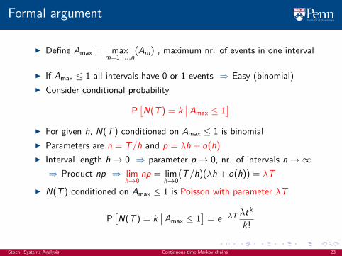
Formal argument

I Define Amax = maxm=1,...,n

(Am) , maximum nr. of events in one interval

I If Amax ≤ 1 all intervals have 0 or 1 events ⇒ Easy (binomial)

I Consider conditional probability

P[N(T ) = k

∣∣Amax ≤ 1]

I For given h, N(T ) conditioned on Amax ≤ 1 is binomial

I Parameters are n = T/h and p = λh + o(h)

I Interval length h→ 0 ⇒ parameter p → 0, nr. of intervals n→∞⇒ Product np ⇒ lim

h→0np = lim

h→0(T/h)(λh + o(h)) = λT

I N(T ) conditioned on Amax ≤ 1 is Poisson with parameter λT

P[N(T ) = k

∣∣Amax ≤ 1]

= e−λTλtk

k!


Formal argument (continued)

I Separate study in Amax ≤ 1 and Amax > 1. That is, condition

P [N(T ) = k] = P[N(T ) = k

∣∣Amax ≤ 1]P [Amax ≤ 1]

+ P[N(T ) = k

∣∣Amax > 1]P [Amax > 1]

I Property (iii) implies that P [Amax > 1] vanishes as h→ 0

P [Amax > 1] ≤n∑

m=1

P [Am > 1] = no(h) = To(h)

h→ 0

I Thus, as h→ 0, P [Amax > 1]→ 0 and P [Amax ≤ 1]→ 1. Then

limh→0

P [N(T ) = k] = limh→0

P[N(T ) = k

∣∣Amax ≤ 1]

I Latter is, as already seen, Poisson

⇒ Then N(T ) Poisson with parameter λT









Limit probabilities


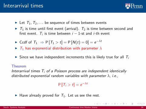
Interarrival times

I Let T1,T2, . . . be sequence of times between events

I T1 is time until first event (arrival). T2 is time between second andfirst event. Ti is time between i − 1-st and i-th event

I Ccdf of T1 ⇒ P [T1 > t] = P [N(t) = 0] = e−λt

I T1 has exponential distribution with parameter λ

I Since we have independent increments this is likely true for all Ti

TheoremInterarrival times Ti of a Poisson process are independent identicallydistributed exponential random variables with parameter λ, i.e.,

P [Ti > t] = e−λt

I Have already proved for T1. Let us see the rest.


Interarrival times

Proof.

I Let Si be absolute time of i-th event. Condition on Si

P [Ti+1 > t] =

∫P[Ti+1 > t

∣∣Si = s]

P [Si = s] ds

I To have Ti+1 > t given that Si = s it must be N(s + t) = N(s)

P[Ti+1 > t

∣∣Si = s]

= P[N(t + s)− N(s) = 0

∣∣N(s)]

I Since increments are independent conditioning on N(s) is moot

P[Ti+1 > t

∣∣Si = s]

= P [N(t + s)− N(s) = 0]

I Since increments are also stationary the latter is

P[Ti+1 > t

∣∣Si = s]

= P [N(t) = 0] = e−λt

I Substituting into integral yields ⇒ P [Ti+1 > t] = e−λt


Alternative definition of Poisson process

I Start with sequence of independent random times T1,T2, . . .

I Times Ti ∼ exp(λ) have exponential distribution with parameter λ

I Define time of i-th event Si

Si = T1 + T2 + . . .+ Ti

I Define counting process ofevents happening at Si

N(t) = maxi

(Si ≤ t)

I N(t) is a Poisson processt

N(t)

1

2

3

4

5

6

S1 S2 S3 S4 S5 S6

T1T2 T3 T4 T5T6

I If N(t) is a Poisson process interarrival times Ti are exponential

I To show that definition is equivalent have to show the converse

I I.e., if interarrival times are exponential, process is Poisson


Alternative definition of Poisson process (cont.)

I Exponential i.i.d interarrival times ⇒ Poisson process?

I Show that implies definition (i)-(iii)

I Stationary true because all Ti have same distribution

I Independent increments true because interarrival times areindependent and exponential RVs are memoryless

I Can have more than two events in (0, h] only if T1 < h and T2 < h

P [N(h) > 1] ≤ P [T1 ≤ h] P [T2 ≤ h]

= (1− e−λh)2 = (λh)2 + o(h2) = o(h)

I We have no event in (0, h] if T1 > h

P [N(h) = 0] = P [T1 ≥ h] = e−λh = 1− λh + o(h)

I The remaining case is N(h) = 1 whose probability is

P [N(h) = 1] = 1− P [N(h) = 0]− P [N(h) > 1] = λh + o(h)


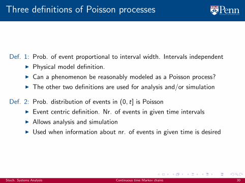
Three definitions of Poisson processes

Def. 1: Prob. of event proportional to interval width. Intervals independent

I Physical model definition.

I Can a phenomenon be reasonably modeled as a Poisson process?

I The other two definitions are used for analysis and/or simulation

Def. 2: Prob. distribution of events in (0, t] is Poisson

I Event centric definition. Nr. of events in given time intervals

I Allows analysis and simulation

I Used when information about nr. of events in given time is desired


Three definitions of Poisson processes (continued)

Def. 3: Prob. distribution of interarrival times is exponential

I Time centric definition. Times at which events happen

I Allows analysis and simulation.

I Used when information about event times is of interest

Obs: Restrictions in Def. 1 are mild, yet they impose a lot of structure asimplied by Defs. 2 & 3


Example: Number of visitors to a web page

I Nr. of unique visitors to a webpage between 6:00pm to 6:10pm

Def 1: Poisson process? Probability proportional to time interval andindependent intervals seem reasonable assumptions

I Model as Poisson process with rate λ visits/second (v/s)

Def 2: Arrivals in interval of duration t are Poisson with parameter λt

I Expected nr. of visits in 10 minutes? ⇒ E [N(600)] = 600λ

I Prob. of exactly 10 visits in 1 sec? ⇒ P [N(1) = 10] = e−λλ/10!

I Data shows N average visits in 10 minutes (600s). Approximate λ

⇒ Since E [N(600)] = 600λ can make λ̂ = N/600


Number of visitors to a web page (continued)

Def 3: Interarrival times Ti are exponential with parameter λ

I Expected time between visitors? ⇒ E [Ti ] = 1/λ

I Expected arrival time Sn of n-th visitor?

⇒ Can write time Sn as sum of Ti , i.e., Sn =∑n

i=1 Ti .

⇒ Taking expected value E [Sn] =∑n

i=1 E [Ti ] = n/λ









Limit probabilities


Definition

I Continuous time positive variable t ∈ R+

I States X (t) taking values in countable set, e.g., 0, 1, . . . , i , . . .

I Stochastic process X (t) is a continuous time Markov chain (CTMC) if

P[X (t + s) = j

∣∣X (s) = i ,X (u) = x(u), u < s]

= P[X (t + s) = j

∣∣X (s) = i]

I Memoryless property ⇒ The future X (t + s) given the present X (s) isindependent of the past X (u) = x(u), u < s

I In principle need to specify functions P[X (t + s) = j

∣∣X (s) = i]

⇒ For all times t, for all times s and for all pairs of states (i , j)


Notation, homogeneity

I Notation: X [s : t] state values for all times s ≤ u ≤ t, includes borders

I X (s : t) values for all times s < u < t, borders excluded

I X (s : t] values for all times s < u ≤ t, exclude left, include right

I X [s : t) values for all times s ≤ u < t, include left, exclude right

I Homogeneous CTMC if P[X (t + s) = j

∣∣X (s) = i]

constant for all s

I Still need P[X (t + s) = j

∣∣X (s) = i]

for all t and pairs (i , j)

I We restrict consideration to homogeneous CTMCs

I Memoryless property makes it somewhat simpler


Transition times

I Ti = time until transition out of state i into any other state j

I Ti is a RV called transition time with cdf

P [Ti > t] = P[X (0 : t] = i

∣∣X (0) = i]

I Probability of Ti > t + s given that Ti > s? Use cdf expression

P[Ti > t + s

∣∣Ti > s]

= P[X (0 : t + s] = i

∣∣X [0 : s] = i]

= P[X (s : t + s] = i

∣∣X [0 : s] = i]

= P[X (s : t + s] = i

∣∣X (s) = i]

= P[X (0 : t] = i

∣∣X (0) = i]

I Equalities true because: Already observed that X [0 : s] = i .Memoryless property. Homogeneity

I From cdf expression ⇒ P[Ti > t + s

∣∣Ti > s]

= P [Ti > t]

I Transition times are exponential RVs


Alternative definition

I Exponential transition times is a fundamental property of CTMCs

I Can be used as “algorithmic” definition of CTMCs

I Continuous times stochastic process X (t) is a CTMC if

I Transition times Ti are exponential RVs with mean 1/νiI When they occur, transitions out of i are into j with probability Pij

∞∑j=1

Pij = 1, Pii = 0

I Transition times Ti and transitioned state j are independent

I Define matrix P grouping transition probabilities Pij

I CTMC states evolve as a discrete time MC

I State transitions occur at random exponential intervals Ti ∼ exp(νi )

I As opposed to occurring at fixed intervals


Embedded discrete time MCs

DefinitionConsider a CTMC with transition probs. P and rates νi . The (discretetime) MC with transition probs. P is the CTMC’s embedded MC

I Transition probabilities P describe a discrete time MC

I States do not transition into themselves (Pii = 0, P’s diagonal null)

I Can use underlying discrete time MCs to understand CTMCs

I Accesibility: State j is accessible from state i if it is accessible in thediscrete time MC with transition probability matrix P

I Communication: States i and j communicate if they communicate inthe discrete time MC with transition probability matrix P

I Communication is a class property. Proof: It is for discrete time MC

I Recurrent/Transient. Recurrence is class property. Etc. More later


Transition rates

I Expected value of transition time Ti is E [Ti ] = 1/νiI Can interpret νi as the rate of transition out of state i

I Of these transitions, Pij of them are into state j

I Can interpret qij := νiPij as transition rate from i to j . Define so

I Transition rates are yet another specification of CTMC

I If qij are given can recover νi as

νi = νi

∞∑j=1,j 6=i

Pij =∞∑

j=1,j 6=i

νiPij =∞∑

j=1,j 6=i

qij

I And can recover Pij as ⇒ Pij = qij/νi = qij

( ∞∑j=1,j 6=i

qij

)−1


Example: Birth and death processes

I State X (t) = 0, 1, . . . Interpret as number of individuals

I Birth and deaths occur at state-dependent rates. When X (t) = i

I Births ⇒ individuals added at exponential times with mean 1/λi

⇒ birth or arrival rate = λi births per unit of time

I Deaths ⇒ individuals removed at exponential times with rate 1/µi

⇒ death or departure rate = µi births per unit of time

I Birth and death times are independent

I As are subsequent birth and death processes

I Birth and death (BD) processes are then CTMC


Transition times and probabilities

I Transition times. Leave state i 6= 0 when birth or death occur

I If TB and TD are times to next birth and death, Ti = min(TB ,TD)

I Since TB and TD are exponential, so is Ti with rate

νi = λi + µi

I When leaving state i can go to i + 1 (birth first) or i − 1 (death first)

I Birth occurs before death with probability ⇒ λiλi + µi

= Pi,i+1

I Death occurs before birth with probability ⇒ µi

λi + µi= Pi,i−1

I Leave state 0 only if a birth occurs (it at all) then

ν0 = λ0 P01 = 1

I If leaves 0, goes to 1 with probability 1. Might not leave 0 if λ0 =∞


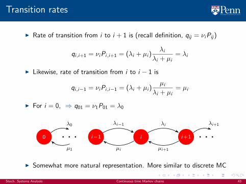
Transition rates

I Rate of transition from i to i + 1 is (recall definition, qij = νiPij)

qi,i+1 = νiPi,i+1 = (λi + µi )λi

λi + µi= λi

I Likewise, rate of transition from i to i − 1 is

qi,i−1 = νiPi,i−1 = (λi + µi )µi

λi + µi= µi

I For i = 0, ⇒ q01 = ν1P01 = λ0

i i+1i−10

λi

µi µi+1

λi−1λ0 λi+1

µ1

. . . . . .

I Somewhat more natural representation. More similar to discrete MC


M/M/1 queue

I A M/M/1 queue is a BD process with λi = λ and µi = µ constant

I Customers arrive for service at a rate of λ per unit of time

I They are serviced at a rate of µ customers per time unit

i i+1i−10

λ

µ µ

λλ λ

µ

. . . . . .

I The M/M is for Markov arrivals / Markov departures

I The 1 is because there is only one server









Limit probabilities


Definition

I Two equivalent ways of specifying a CTMC

I Transition time averages 1/νi + Transition probabilities Pij

I Easier description. Typical starting point for CTMC modeling

I Transition prob. function ⇒ Pij(t) := P[X (t + s) = j

∣∣X (s) = i]

I More complete description

I Compute transition prob. function from transition times and probs.

I Notice two obvious properties Pij(0) = 1, Pii (0) = 1


Roadmap to determine Pij(t)

I Goal is to obtain a differential equation whose solution is Pij(t)

I For that, need to study change in Pij(t) when time changes slightly

I Separate in two subproblems

⇒ Transition probabilities for small time h, Pij(h)

⇒ Transition probabilities in t + h as function of those in t and h

I We can combine both results in two different ways

I Jump from 0 to t then to t + h ⇒ Process runs a little longer

I Changes where the process is going to ⇒ Forward equations

I Jump from 0 to h then to t + h ⇒ Process starts a little later

I Changes where the process comes from ⇒ Backward equations


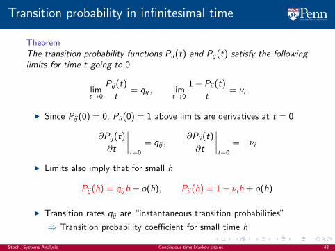
Transition probability in infinitesimal time

TheoremThe transition probability functions Pii (t) and Pij(t) satisfy the followinglimits for time t going to 0

limt→0

Pij(t)

t= qij , lim

t→0

1− Pii (t)

t= νi

I Since Pij(0) = 0, Pii (0) = 1 above limits are derivatives at t = 0

∂Pij(t)

∂t

∣∣∣∣t=0

= qij ,∂Pii (t)

∂t

∣∣∣∣t=0

= −νi

I Limits also imply that for small h

Pij(h) = qijh + o(h), Pii (h) = 1− νih + o(h)

I Transition rates qij are “instantaneous transition probabilities”

⇒ Transition probability coefficient for small time h


Transition probability in infinitesimal time (proof)

Proof.

I Consider a small time h

I Since 1− Pii is the probability of transitioning out of state i

1− Pii (h) = P [Ti < h] = νih + o(h)

I Divide by h and take limit

I For Pij(t) notice that since two or more transitions have o(h) prob

Pij(h) = P[X (h) = j

∣∣X (0) = i]

= PijP [Ti ≤ h] + o(h)

I Since Ti is exponential P [Ti ≤ h] = νih + o(h). Then

Pij(h) = νiPij + o(h) = qijh + o(h)

I Divide by h and take limit


Chapman-Kolmogorov equations

TheoremFor all times s and t the transition probability functions Pij(t + s) areobtained from Pik(t) and Pkj(s) as

Pij(t + s) =∞∑k=0

Pik(t)Pkj(s)

I As for discrete time MC, to go from i to j in time t + s

⇒ Go from i to a certain k at time t ⇒ Pik(t)

⇒ In the remaining time s go from k to j ⇒ Pkj(s)

⇒ Sum over all possible intermediate steps k


Chapman-Kolmogorov equations (proof)

Proof.

Pij(t + s)

= P[X (t + s) = j

∣∣X (0) = i]

Definition of Pij(t + s)

=∞∑k=0

P[X (t + s) = j

∣∣X (t) = k,X (0) = i]P[X (t) = k

∣∣X (0) = i]

Sum of conditional probabilities

=∞∑k=0

P[X (t + s) = j

∣∣X (t) = k]Pik(t) Memoryless property of CTMC

and definition of Pik(t)

=∞∑k=0

P[X (s) = j

∣∣X (0) = k]Pik(t) Time invariance / homogeneity

=∞∑k=0

Pkj(s)Pik(t) Definition of Pkj(s)


Combining both results

I Let us combine the last two results to express Pij(t + h)

I Use Chapman-Kolmogorov’s equations for 0→ t → h

Pij(t + h) =∞∑k=0

Pik(t)Pkj(h) = Pij(t)Pjj(h) +∞∑

k=0,k 6=i

Pik(t)Pkj(h)

I Use infinitesimal time expression

Pij(t + h) = Pij(t)(1− νjh) +∞∑

k=0,k 6=i

Pik(t)qkjh + o(h)

I Subtract Pij(t) from both sides and divide by h

Pij(t + h)− Pij(t)

h= −νjPij(t) +

∞∑k=0,k 6=i

Pik(t)qkj +o(h)

h

I The right hand side is a “derivative” ratio. Let h→ 0


Kolmogorov’s forward equations

TheoremThe transition probability functions Pij(t) of a CTMC satisfy the systemof differential equations (for all pairs i , j)

∂Pij(t)

∂t=

∞∑k=0,k 6=j

qkjPik(t)− νjPij(t)

I ∂Pij(t)/∂t = rate of change of Pij(t)

I qkjPik(t) = (transition into k in 0→ t) ×(rate of moving into j in next instant)

I νjPij(t) = (transition into j in 0→ t) ×(rate of leaving j in next instant)

I Change in Pij(t) =∑

k (moving into j from k)− (leaving j)

I Kolmogorov’s forward equations valid in most cases, but not always


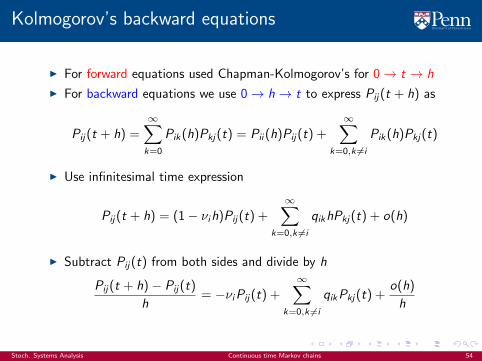
Kolmogorov’s backward equations

I For forward equations used Chapman-Kolmogorov’s for 0→ t → h

I For backward equations we use 0→ h→ t to express Pij(t + h) as

Pij(t + h) =∞∑k=0

Pik(h)Pkj(t) = Pii (h)Pij(t) +∞∑

k=0,k 6=i

Pik(h)Pkj(t)

I Use infinitesimal time expression

Pij(t + h) = (1− νih)Pij(t) +∞∑

k=0,k 6=i

qikhPkj(t) + o(h)

I Subtract Pij(t) from both sides and divide by h

Pij(t + h)− Pij(t)

h= −νiPij(t) +

∞∑k=0,k 6=i

qikPkj(t) +o(h)

h


Kolmogorov’s backward equations

TheoremThe transition probability functions Pij(t) of a CTMC satisfy the systemof differential equations (for all pairs i , j)

∂Pij(t)

∂t=

∞∑k=0,k 6=i

qikPkj(t)− νiPij(t)

I νiPij(t) = (transition into j in h→ t) ×(do not do that if leave i in initial instant)

I qikPkj(t) = (rate of transition into k in 0→ h) ×(transition from k into j in h→ t)

I Forward equations ⇒ change in Pij(t) if finish h later

I Backward equations ⇒ change in Pij(t) if start h later

I Where process goes (forward) ⇔ where process comes from (backward)









Limit probabilities


A CTMC with two states

I Simplest possible CTMC has only two states. Say 0 and 1

I Transition rates are q01 and q10I Given transition rates can find

mean transition times as

ν0 =∑j 6=0

q0i = q01 ν1 =∑j 6=1

q1i = q10

0 1

q01

q10

I Use Kolmogorov’s equations to find transition probability functions

P00(t), P01(t), P10(t), P11(t)

I Note that transition probs. out of each state sum up to one

P00(t) + P01(t) = 1 P10(t) + P11(t) = 1


Kolmogorov’s forward equations

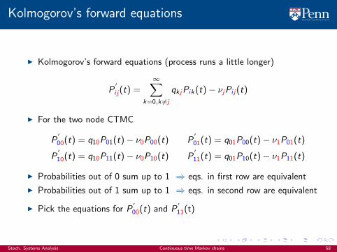
I Kolmogorov’s forward equations (process runs a little longer)

P′

i j(t) =∞∑

k=0,k 6=j

qkjPik(t)− νjPi j(t)

I For the two node CTMC

P′

00(t) = q10P01(t)− ν0P00(t) P′

01(t) = q01P00(t)− ν1P01(t)

P′

10(t) = q10P11(t)− ν0P10(t) P′

11(t) = q01P10(t)− ν1P11(t)

I Probabilities out of 0 sum up to 1 ⇒ eqs. in first row are equivalent

I Probabilities out of 1 sum up to 1 ⇒ eqs. in second row are equivalent

I Pick the equations for P′

00(t) and P′

11(t)


Solution of backward equations

I Use ⇒ Relation between transition rates: ν0 = q01 and ν1 = q10⇒ Probs. sum 1: P01(t) = 1− P00(t) and P01(t) = 1− P00(t)

P′

00(t) = q10[1− P00(t)

]− q01P00(t) = q10 − (q10 + q01)P00(t)

P′

11(t) = q01[1− P11(t)

]− q10P11(t) = q01 − (q10 + q01)P11(t)

I Can obtain exact same pair of equations from backward equations

I First order linear differential equations. Solutions are exponential

I For P00(t) propose candidate solution (just take derivate to check)

P00(t) =q10

q10 + q01+ ce−(q10+q01)t

I To determine c use initial condition P00(t) = 1


Solution of backward equations (continued)

I Evaluation of candidate solution at initial condition P00(t) = 1 yields

1 =q10

q10 + q01+ c ⇒ c =

q01q10 + q01

I Finally transition probability function P00(t)

P00(t) =q10

q10 + q01+

q01q10 + q01

e−(q10+q01)t

I Repeat for P11(t). Same exponent, different constants

P11(t) =q01

q10 + q01+

q10q10 + q01

e−(q10+q01)t

I As time goes to infinity, P00(t) and P11(t) converge exponentially

I Convergence rate depends on magnitude of q10 + q01


Convergence of transition probabilities

I Recall P01 = 1− P00 and P10 = 1− P11. Steady state distributions

limt→∞

P00(t) =q10

q10 + q01limt→∞

P01(t) =q01

q10 + q01

limt→∞

P11(t) =q01

q10 + q01limt→∞

P10(t) =q10

q10 + q01

I Limit distribution exists and is independent of initial condition

⇒ Compare across diagonals


Kolmogorov’s forward equations in matrix form

I Restrict attention to finite CTMCs with N states

I Define matrix R ∈ RN×N with elements rij = qij , rii = −νi .

I Rewrite Kolmogorov’s forward eqs. as (process runs a little longer)

P′ij(t) =

N∑k=1,k 6=j

qkjPik(t)− νjPij(t) =N∑

k=1

rkjPik(t)

I Right hand side defines elements of a matrix product

P11(t) · P1k (t) · P1N (t)

· · · · ·Pi1(t) · Pik (t) · PiN (t)

· · · · ·PN1(t) · PNk (t) · PJN (t)

r11 · r1j · r1N

· · · · ·rk1 · rkj · rkN

· · · · ·rN1 · rNj · rNN

s11 · s1j · s1N

· · · · ·si1 · sij · siN

· · · · ·sN1 · sNk · sNN

P(t) =

= R

= P(t)R = P′(t)


Kolmogorov’s backward equations in matrix form

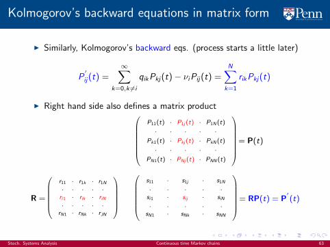
I Similarly, Kolmogorov’s backward eqs. (process starts a little later)

P′

ij(t) =∞∑

k=0,k 6=i

qikPkj(t)− νiPij(t) =N∑

k=1

rikPkj(t)

I Right hand side also defines a matrix product

r11 · r1k · r1N· · · · ·ri1 · rik · riN· · · · ·

rN1 · rNk · rJN

P11(t) · P1j (t) · P1N (t)

· · · · ·Pk1(t) · Pkj (t) · PkN (t)

· · · · ·PN1(t) · PNj (t) · PNN (t)

s11 · s1j · s1N

· · · · ·si1 · sij · siN

· · · · ·sN1 · sNk · sNN

R =

= P(t)

= RP(t) = P′(t)


Kolmogorov’s equations in matrix form

I Matrix form of Kolmogorov’s forward equation ⇒ P′(t) = P(t)R

I Matrix form of Kolmogorov’s backward equation ⇒ P′(t) = RP(t)

⇒ More similar than apparent

⇒ But not equivalent because matrix product not commutative

I Notwithstanding both equations have to accept the same solution


Matrix exponential

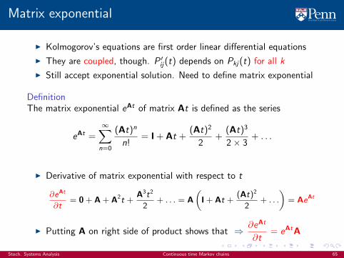
I Kolmogorov’s equations are first order linear differential equations

I They are coupled, though. P ′ij(t) depends on Pkj(t) for all k

I Still accept exponential solution. Need to define matrix exponential

DefinitionThe matrix exponential eAt of matrix At is defined as the series

eAt =∞∑n=0

(At)n

n!= I + At +

(At)2

2+

(At)3

2× 3+ . . .

I Derivative of matrix exponential with respect to t

∂eAt

∂t= 0 + A + A2t +

A3t2

2+ . . . = A

(I + At +

(At)2

2+ . . .

)= AeAt

I Putting A on right side of product shows that ⇒ ∂eAt

∂t= eAtA


Solution of Kolmogorov’s equations

I Propose solution of the form P(t) = eRt

I P(t) solves backward equations. Derivative with respect to time is

∂P(t)

∂t=∂eRt

∂t= ReRt = RP(t)

I It also solves forward equations

∂P(t)

∂t=∂eRt

∂t= eRtR = P(t)R

I Also notice that P(0) = I. As it should (Pii (0) = 1, and Pij(0) = 0)


Unconditional probabilities

I P(t) is transition prob. from states at time 0 to states at time t

I Define unconditional probs. at time t, pj(t) := P [X (t) = i ]

I Group in vector p(t) = [p1(t), p2(t), . . . , pj(t), . . .]T

I Given initial distribution p(0) find pj(t) conditioning on initial state

pj(t) =∞∑i=0

P[X (t) = j

∣∣X (0) = i]

P [X (0) = i ] =∞∑i=0

Pij(t)pi (0)

I Using matrix-vector notation ⇒ p(t) = PT (t)p(0)


Limit probabilities







Limit probabilities


Recurrent and transient states

I Recall the embedded discrete time MC associated with any CTMC

I Transition probs. of MC form the matrix P of the CTMC

I States do not transition into themselves (Pii = 0, P’s diagonal null)

I States i ↔ j communicate in the CTMC if i ↔ j in the MC

I Communication partitions MC in classes ⇒ induces CTMC partition

I CTMC is irreducible if embedded MC contains a single class

I State i is recurrent if i is recurrent in the embedded MC

I State i is transient if i is transient in the embedded MC

I State i is positive recurrent if i is so in the embedded MC

I Transience and recurrence shared by elements of a MC class

⇒ Transience and recurrence are class properties of CTMC

I Periodicity not possible in CTMCs


Limit probabilities

TheoremConsider irreducible positive recurrent CTMC with transition rates νi andqij . Then, limt→∞ Pij(t) exists and is independent of the initial state i ,i.e.,

Pj = limt→∞

Pij(t) exists for all i

Furthermore, steady state probabilities Pj ≥ 0 are the unique nonnegativesolution of the system of linear equations

νjPj =∞∑

k=0,k 6=j

qkjPk ,

∞∑j=0

Pj = 1

I Limit distribution exists and is independent of initial condition

I Obtained as solution of system of linear equations

I Analogous to MCs. Algebraic equations slightly different


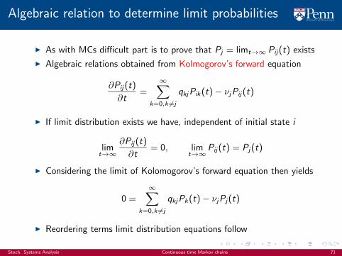
Algebraic relation to determine limit probabilities

I As with MCs difficult part is to prove that Pj = limt→∞ Pij(t) exists

I Algebraic relations obtained from Kolmogorov’s forward equation

∂Pij(t)

∂t=

∞∑k=0,k 6=j

qkjPik(t)− νjPij(t)

I If limit distribution exists we have, independent of initial state i

limt→∞

∂Pij(t)

∂t= 0, lim

t→∞Pij(t) = Pj(t)

I Considering the limit of Kolomogorov’s forward equation then yields

0 =∞∑

k=0,k 6=j

qkjPk(t)− νjPj(t)

I Reordering terms limit distribution equations follow


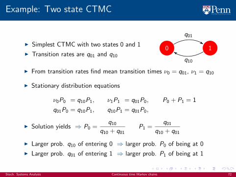
Example: Two state CTMC

I Simplest CTMC with two states 0 and 1

I Transition rates are q01 and q100 1

q01

q10

I From transition rates find mean transition times ν0 = q01, ν1 = q10

I Stationary distribution equations

ν0P0 = q10P1, ν1P1 = q01P0, P0 + P1 = 1

q01P0 = q10P1, q10P1 = q01P0,

I Solution yields ⇒ P0 =q10

q10 + q01P1 =

q01q10 + q01

I Larger prob. q10 of entering 0 ⇒ larger prob. P0 of being at 0

I Larger prob. q01 of entering 1 ⇒ larger prob. P1 of being at 1


Ergodicity

I Consider the fraction Ti (t) of time spent in state i up to time t

Ti (t) :=1

t

∫ t

0

I {X (t) = i}

I Ti (t) = time/ergodic average. Its limit limt→∞

Ti (t) is ergodic limit

I If CTMC is irreducible, positive recurrent ergodicity holds

Pi = limt→∞

Ti (t) = limt→∞

1

t

∫ t

0

I {X (t) = i} a.s.

I Ergodic limit coincides with limit probabilities (almost surely)


Ergodicity (continued)

I Consider function f (i) associated with state i . Can write f(X (t)

)as

f(X (t)

)=∞∑i=1

f (i)I {X (t) = i}

I Consider the time average of the function of the state f(X (t)

)limt→∞

1

t

∫ t

0

f(X (t)

)= lim

t→∞

1

t

∫ t

0

∞∑i=1

f (i)I {X (t) = i}

I Interchange summation with integral and limit to say

limt→∞

1

t

∫ t

0

f(X (t)

)=∞∑i=1

f (i) limt→∞

1

t

∫ t

0

I {X (t) = i} =∞∑i=1

f (i)Pi

I Function’s ergodic limit = functions limit average value


Limit distribution equations as balance equations

I Reconsider limit distribution equations ⇒ νjPj =∞∑

i=0,k 6=j

qkjPk

I Pj = fraction of time spent in state j

I νj = rate of transition out of state j given CTMC is in state j

⇒ νjPj = rate of transition out of state j (unconditional)

I qkj = rate of transition from k to j given CTMC is in state k

⇒ qkjPk = rate of transition from k to j (unconditional)

⇒∑∞

i=0,k 6=j qkjPk = rate of transition into j , from all states

I Rate of transition out of state j = rate of transition into j

I Balance equations ⇒ Balance nr. of transitions in and out of state j


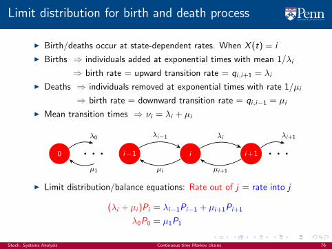
Limit distribution for birth and death process

I Birth/deaths occur at state-dependent rates. When X (t) = i

I Births ⇒ individuals added at exponential times with mean 1/λi

⇒ birth rate = upward transition rate = qi,i+1 = λiI Deaths ⇒ individuals removed at exponential times with rate 1/µi

⇒ birth rate = downward transition rate = qi,i−1 = µi

I Mean transition times ⇒ νi = λi + µi

i i+1i−10

λi

µi µi+1

λi−1λ0 λi+1

µ1

. . . . . .

I Limit distribution/balance equations: Rate out of j = rate into j

(λi + µi )Pi = λi−1Pi−1 + µi+1Pi+1

λ0P0 = µ1P1


Finding solution of balance equations

I Start expressing all probabilities in terms of P0

I Equation for P0 λ0P0 = µ1P1

I Sum eqs. for P1

and P0λ0P0

(λ1 + µ1)P1

=

=

µ1P1

λ0P0 + µ2P2

λ1P1 = µ2P2

I Sum result andeq. for P2

λ1P1

(λ2 + µ2)P2

=

=

µ2P2

λ1P1 + µ3P3

λ2P2 = µ3P3

...

I Sum result andeq. for Pi

λi−1Pi−1

(λi + µi )Pi

=

=

µiPi

λi−1Pi−1 + µi+1Pi+1

λiPi = µi+1Pi+1


Finding solution of balance equations (continued)

I Recursive substitutions on equations on the left

P1 =λ0µ1

P0

P2 =λ1µ2

P1 =λ1λ0µ2µ1

P0

P3 =λ2µ3

P2 =λ2λ1λ0µ3µ2µ1

P0

...

Pi+1 =λiµi+1

Pi =λiλi−1 . . . λ0µi+1µi . . . µ0

P0

I To find P0 use∑∞

i=0 Pi = 1 ⇒ 1 = P0 +∞∑i=0

λiλi−1 . . . λ0µi+1µi . . . µ0

P0


Date post:	27-Sep-2018
Category:	Documents
Upload:	lyliem
View:	221 times
Download:	0 times

Continuous time Markov chains - Penn Engineeringese303/block_3_continuous_time... · Systems...

Documents