Continuous-time Markov chains

Books

- Performance Analysis of Communications Networks and Systems

(Piet Van Mieghem), Chap. 10

- Introduction to Stochastic Processes (Erhan Cinlar), Chap. 8

22

Definition

Stationarity of the transition probabilities

is a continuous-time Markov chain if

The state vector with components obeys from which

33

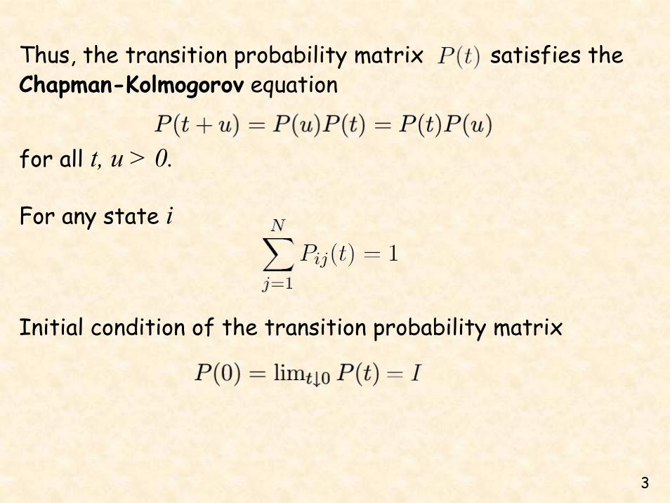
For any state i

Thus, the transition probability matrix satisfies theChapman-Kolmogorov equation

for all t, u > 0.

Initial condition of the transition probability matrix

44

The infinitesimal generator Lemma The transition probability matrix P(t) is continuous for all t≥0.

Additional assumption: the existence of

matrix Q– is called the infinitesimal generator of the continuous-

time Markov process – corresponds to P-I in discrete-time

The sum of the rows in Q is zero, with

and

55

We call qij “rates”• they are derivatives of probabilities and reflect a change in

transition probability from state i towards state j

We define qi = - qii>0. Then,

– Q is bounded if and only if the rates qij are bounded

• It can be shown that qij is always finite.

– For finite-state Markov processes, qj are finite (since qij are finite), but, in general, qj can be infinite.

We consider only CTMCs with all states non-instantaneous

If qj=¶, state j is called instantaneous (when the process enters j, it immediately leaves j)

66

indicates that

For small h

which generalizes the Poisson process and motivates to call qi the rate corresponding to state i

Lemma Given the infinitesimal generator Q, the transition probability matrix P(t) is differentiable for all t≥0, with

the forward equationthe backward equation

77

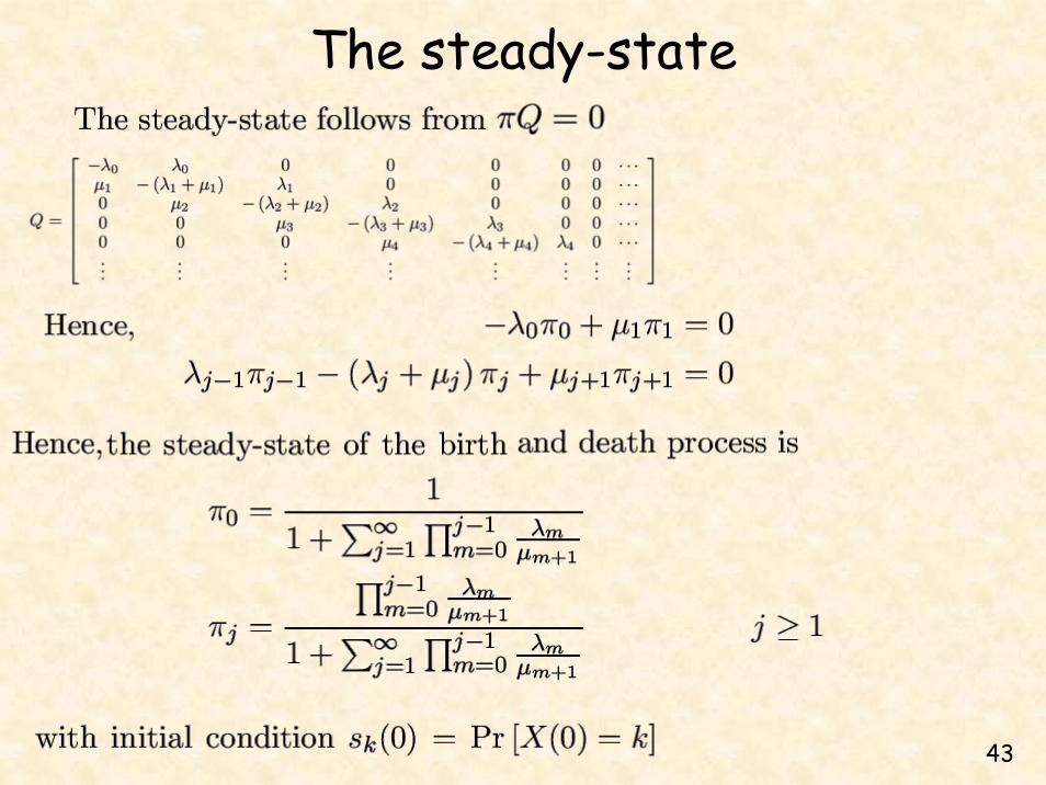
The probability sk(t) that the Markov process is in state kat time t is completely determined by

with initial condition sk(0)

It holds that ï

from which

For and

88

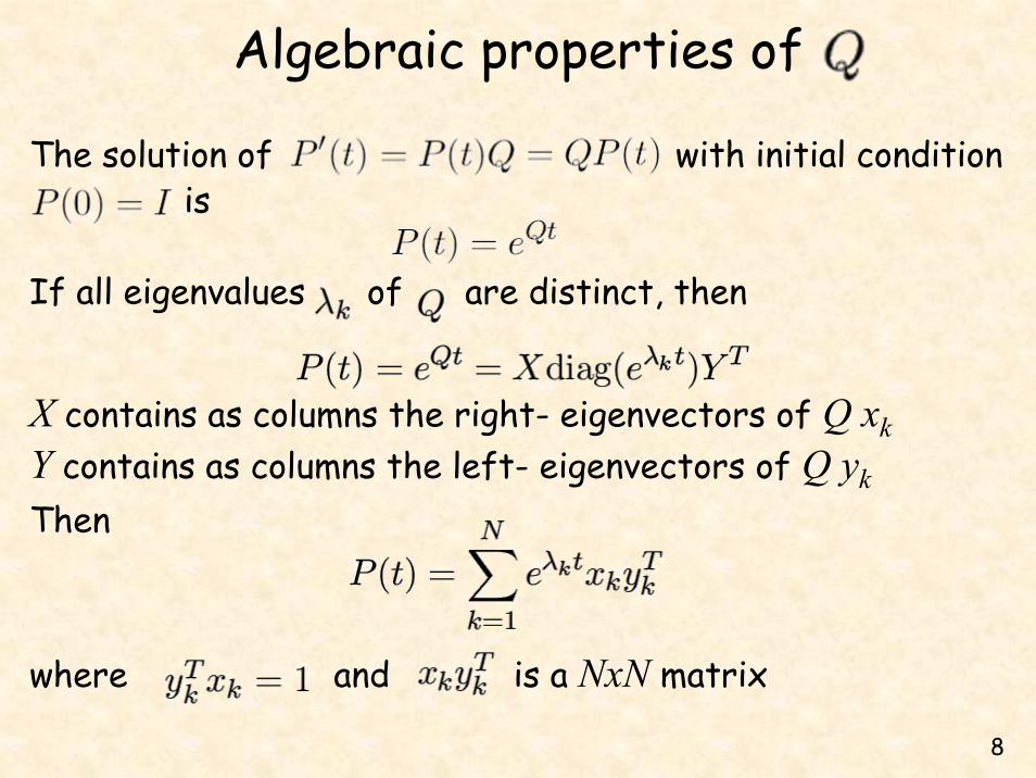
The solution of with initial condition is

If all eigenvalues of are distinct, then

X contains as columns the right- eigenvectors of Q xkY contains as columns the left- eigenvectors of Q ykThen

where and is a NxN matrix

Algebraic properties of

99

Assuming (thus omitting pathological cases) that P(t) is stochastic, irreducible matrix for any time t, we may write

where is the N x N matrix with each row containing the steady-state vector π

spectral or eigendecomposition of the transition probability matrix

Taylor expansion

matrix equivalent of

1010

Exponential sojourn timesTheorem The sojourn times τj of a continuous-time Markov

process in a state j are independent, exponential random variables with mean

Proof • The independence of the sojourn times follows from the

Markov property.• The exponential distribution is proved by demonstrating

that the sojourn times τj satisfy the memoryless property. The only continuous distribution that satisfies the memoryless property is the exponential distribution.

1111

[Cinlar, Ch. 8]

1212

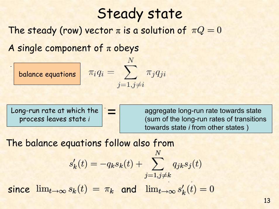
Steady state

A single component of π obeys

For an irreducible, finite-state Markov chain (all states communicate and Pij(t)>0), the steady-state π existsBy definition, the steady-state does not change over time, or . Thus, implies

where

The steady (row) vector π is a solution of

Αll rows of are proportional to the eigenvector of belonging to λ = 0

1313

Steady state

A single component of π obeys

The steady (row) vector π is a solution of

Long-run rate at which the process leaves state i =

balance equations

The balance equations follow also from

since and

aggregate long-run rate towards state (sum of the long-run rates of transitions towards state i from other states )

1414

The embedded Markov chainThe probability that, if a transition occurs, the process

moves from state i to a different state j ≠ i is

For h∞0

Given a transition, it is a transition to another state j ≠ i since

Vij: transition probabilities of the embedded Markov chain

1515

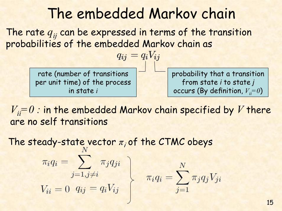
The rate qij can be expressed in terms of the transition probabilities of the embedded Markov chain as

probability that a transition from state i to state j

occurs (By definition, Vii=0)

rate (number of transitions per unit time) of the process

in state i

Vii=0 : in the embedded Markov chain specified by V there are no self transitions

The steady-state vector πi of the CTMC obeys

The embedded Markov chain

1616

The embedded Markov chain

The relations between the steady-state vectors of the CTMC and of its corresponding embedded DTMC are

The classification in the discrete-time case into transient and recurrent can be transferred via the embedded MC to continuous MCs

The steady-state vector υ of the embedded MC obeysi

and

The steady-state vector πi of the CTMC obeys

1717

UniformizationThe restriction that there are no self transitions from a state to itself can be removed

can be rewritten as

or

where and

1818

Uniformizationcan be regarded as a rate matrix with the

property that

(for each state i the transition rate in any state i is precisely the same, equal to β)

can be interpreted as an embedded Markov chain that • allows self transitions and• the rate for each state is equal to β

1919

Uniformization

The transition rates follow fromThe change in transition rates changes

• the steady-state vector (since the balance equations change)

•the number of transitions during some period of time

However, the Markov process is not modified(a self-transition does not change nor the distribution of the time until the next transition to a different state)

2020

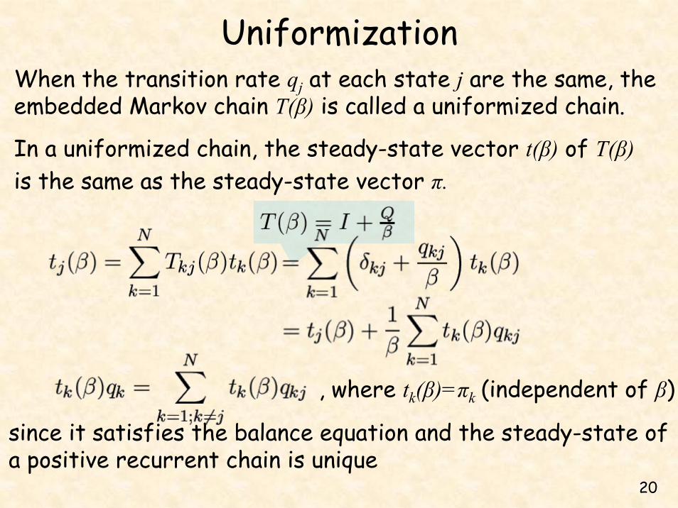
UniformizationWhen the transition rate qj at each state j are the same, the embedded Markov chain T(β) is called a uniformized chain.

Ιn a uniformized chain, the steady-state vector t(β) of T(β)is the same as the steady-state vector π.

, where tk(β)=πk (independent of β)

since it satisfies the balance equation and the steady-state of a positive recurrent chain is unique

2121

Uniformization{Xk(β)}: uniformized (discrete) processN(t): total number of transitions in [0, t] in {Xk(β)}the rates qi=β are all the same ï N(t) is Poisson rate β(for any continuous-time Markov chain, the inter-transition or sojourn

times are i.i.d. exponential random variables)

Prob. that the number oftransitions in [0, t] in {Xk(β)} is k

k-step transition probability of {Xk(β)}

can be interpreted as

2222

Sampled time Markov chain

(are obtained by expanding Pij(t) to first order with fixed step h = Δt)

transition probabilities of thesampled time Markov chain

Approximates the continuous time Markov process

2323

Sampled time Markov chain

is exactly equal to that of the CTMC for any sampling stepby sampling every Δt we miss the smaller-scale dynamics,however the steady-state behavior is exactly captured

The steady-state vector of the sampled-time Markov chain with satisfies for each component j

or

2424

The transitions in a CTMCBased on the embedded Markov chain all properties of the continuous Markov chain may be deduced.

Theorem Let Vij denote the transition probabilities of the embedded Markov chain and qij the rates of the infinitesimalgenerator. The transition probabilities of the corresponding continuous-time Markov chain are found as

2525

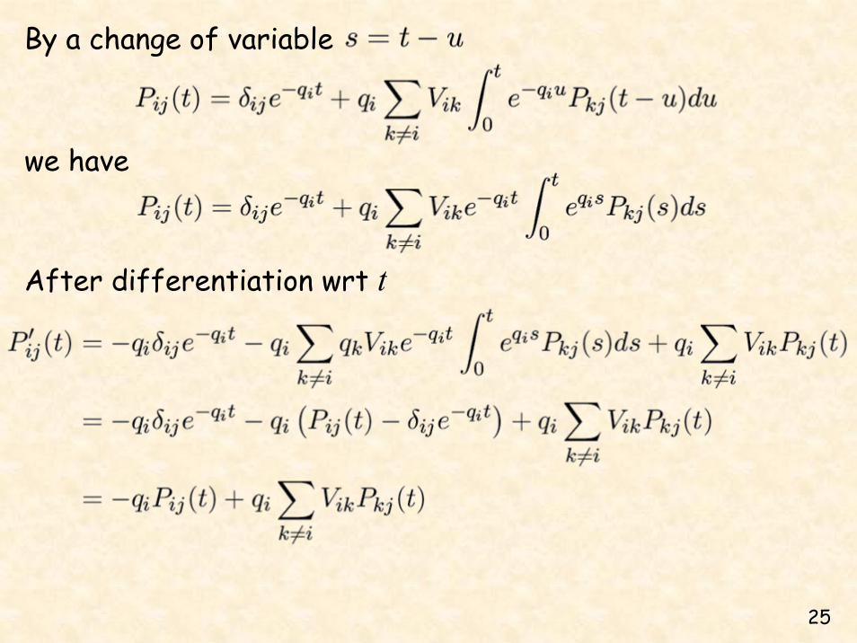
By a change of variable

we have

After differentiation wrt t

2626

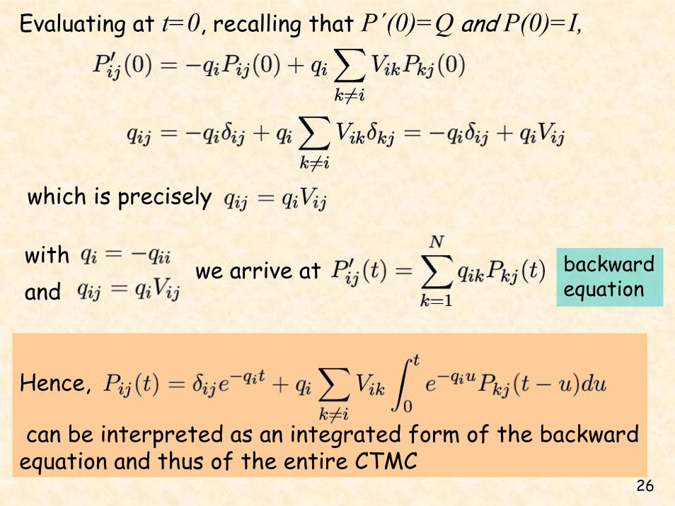
Evaluating at t=0, recalling that P΄(0)=Q and P(0)=I,

backward equation

which is precisely

with

Hence,

can be interpreted as an integrated form of the backward equation and thus of the entire CTMC

andwe arrive at

2727

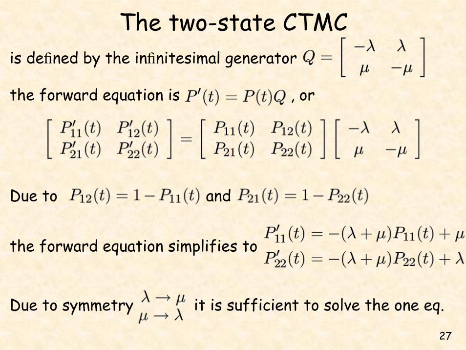
The two-state CTMCis defined by the infinitesimal generator

the forward equation is , or

Due to and

the forward equation simplifies to

Due to symmetry it is sufficient to solve the one eq.

2828

The two-state CTMC

Thus, the solution of is of the form

μ λ μλ μ

− +++

( ) ( )

tc e

The solution of y'(x) + p(x)y(x) = r(x) is of the form

where κ is the constant of integration, and

The constant c follows from the initial conditionï

and

Thus,

2929

For time reversible MCs any vector x satisfying and is a steady state vector

Time reversibilityErgodic MCs with non-zero steady-state distributionSuppose the process is in the steady-state and consider the time-reversed process defined by the sequence

Theorem The time-reversed Markov process is a MC.

A MC is said to be time reversible if for all i and j

Condition for time reversibility for all i, j

rate from i→ j rate from j→ i

3030

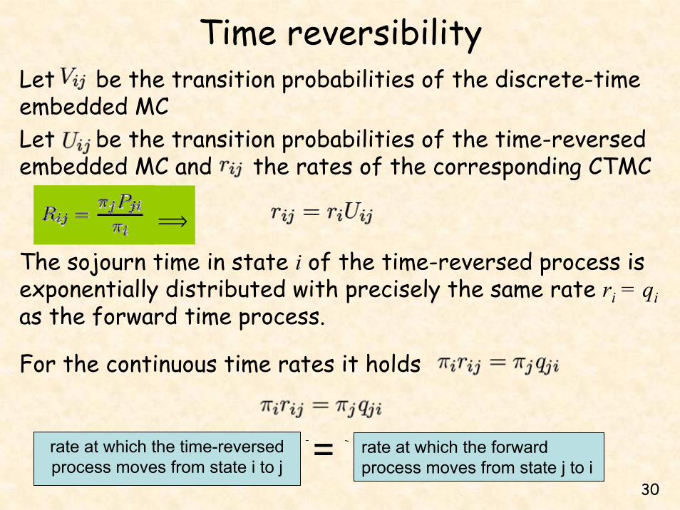
Time reversibilityLet be the transition probabilities of the discrete-time embedded MC Let be the transition probabilities of the time-reversed embedded MC and the rates of the corresponding CTMC

The sojourn time in state i of the time-reversed process is exponentially distributed with precisely the same rate ri = qias the forward time process.

For the continuous time rates it holds

ï

rate at which the time-reversed process moves from state i to j = rate at which the forward

process moves from state j to i

Applications of Markov chains

Books

- Performance Analysis of Communications Networks and Systems

(Piet Van Mieghem), Chap. 11

3232

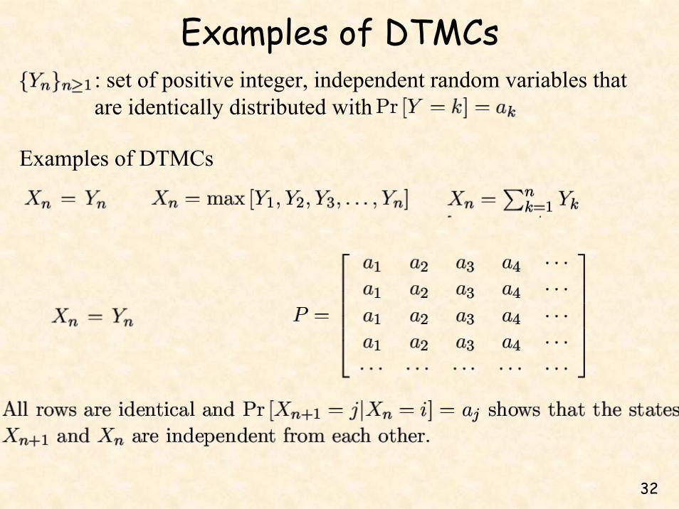
Examples of DTMCs: set of positive integer, independent random variables thatare identically distributed with

Examples of DTMCs

3333

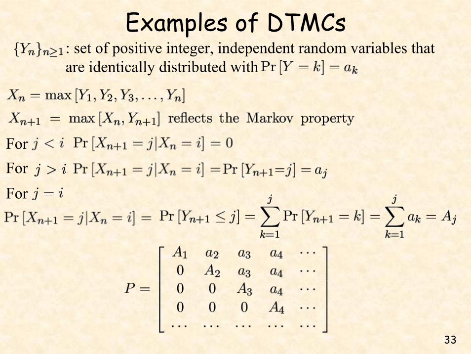
Examples of DTMCs: set of positive integer, independent random variables thatare identically distributed with

For

ForFor

3434

Examples of DTMCs: set of positive integer, independent random variables thatare identically distributed with

For

For

3535

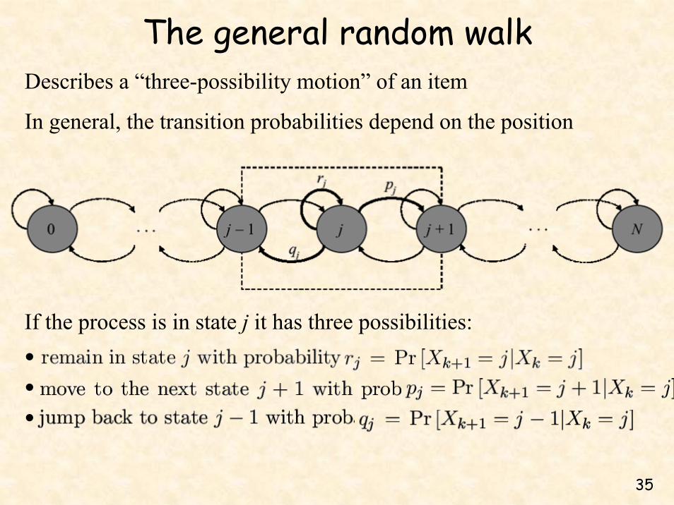
The general random walkDescribes a “three-possibility motion” of an item

In general, the transition probabilities depend on the position

If the process is in state j it has three possibilities:●

●

●

3636

The gambler’s ruin problemA state j reflects the capital of a gambler

– pj is the chance that the gambler wins– qj is the probability that he looses

The gambler – achieves his target when he reaches state N– is ruined at state 0

States 0 and N are absorbing states with r0 = rN = 1In most games pj = p, qj = q and rj = 1-p-q

3737

The probability of gambler’s ruin

or equivalently,

The law of total probability gives

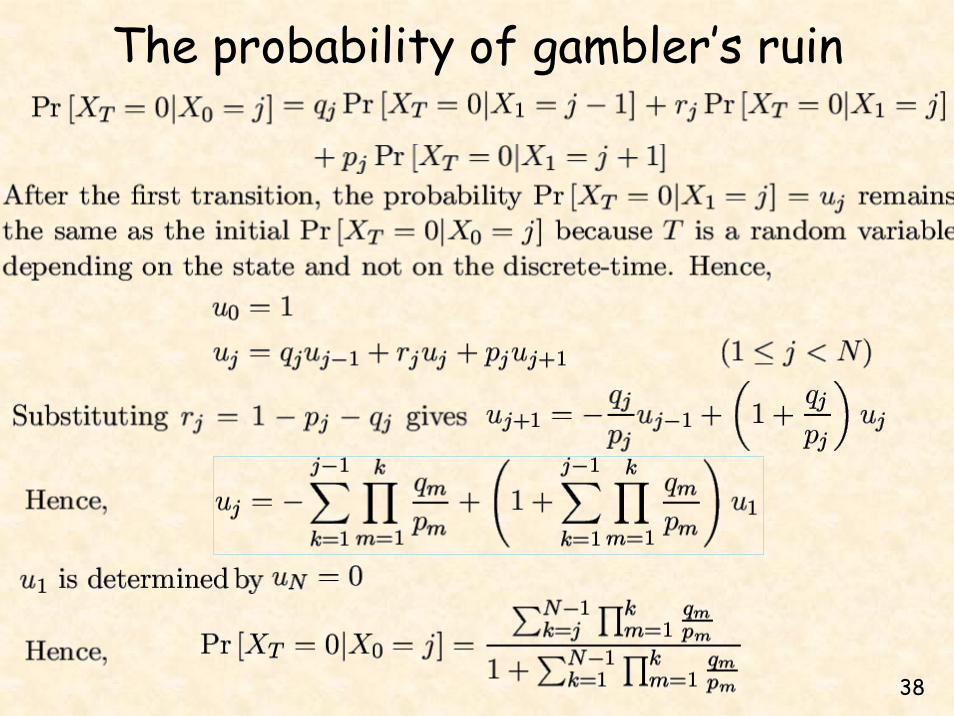
3838

The probability of gambler’s ruin

3939

The probability of gambler’s ruin

4040

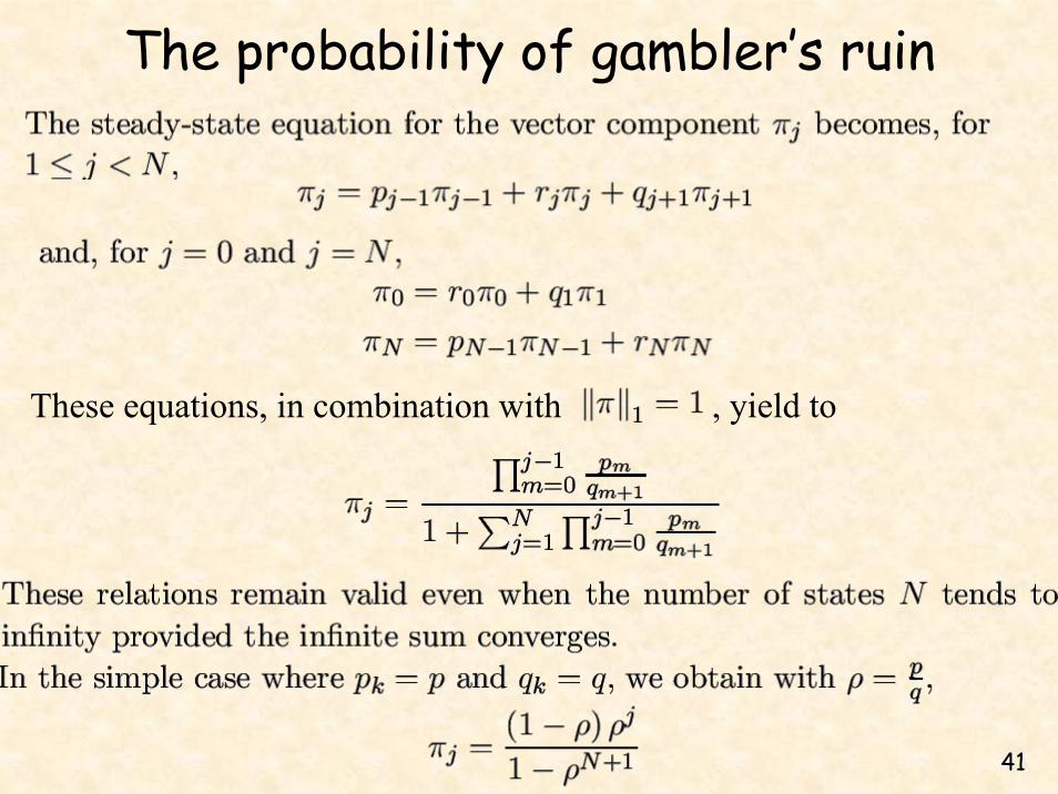
The probability of gambler’s ruinIn the special case where qk = q and pk= p

– The probability of gambler’s ruin becomes

– The mean duration of the game becomes

4141

The probability of gambler’s ruin

These equations, in combination with , yield to

4242

Birth and death process

The embedded Markov chain of the birth and death process is arandom walk with transition probabilities

Differential equations that describe the BD process

4343

The steady-state

4444

The steady-stateThe process is transient if and only if the embedded MC is transient.For a recurrent chain, equals 1(every state j is certainly visited starting from initial state i)For the embedded MC (gambler’s ruin), it holds that

Can be equal to one for only if

Transformed to the birth and death rates

Furthermore, the infinite series must convergeto have a steady-state distribution

•If S1<¶ and S2=¶ the BD process is positive recurrent•If S1=¶ and S2=¶, it is null recurrent•If S2<¶, it is transient

4545

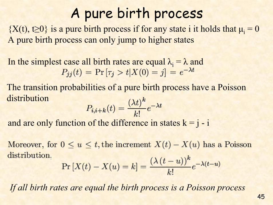
{X(t), t≥0} is a pure birth process if for any state i it holds that μi = 0 A pure birth process can only jump to higher states

In the simplest case all birth rates are equal λi = λ and

A pure birth process

The transition probabilities of a pure birth process have a Poissondistribution

and are only function of the difference in states k = j - i

If all birth rates are equal the birth process is a Poisson process

4646

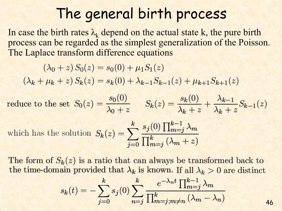
The general birth processIn case the birth rates λk depend on the actual state k, the pure birth process can be regarded as the simplest generalization of the Poisson. The Laplace transform difference equations

4747

The Yule processYule process

Is simplified to

4848

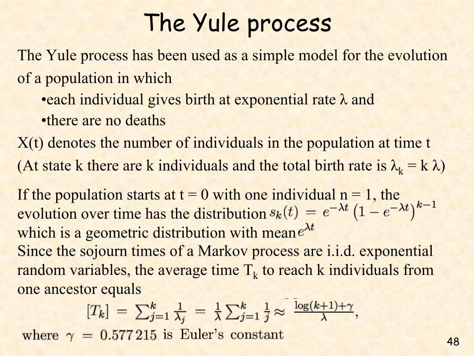
The Yule processThe Yule process has been used as a simple model for the evolution of a population in which

•each individual gives birth at exponential rate λ and•there are no deaths

X(t) denotes the number of individuals in the population at time t(At state k there are k individuals and the total birth rate is λk = k λ)

If the population starts at t = 0 with one individual n = 1, theevolution over time has the distributionwhich is a geometric distribution with meanSince the sojourn times of a Markov process are i.i.d. exponentialrandom variables, the average time Tk to reach k individuals fromone ancestor equals

4949

Constant rate birth and death processIn a constant rate birth and death process, both the birth rate λk = λand death rate μk = μ are constant for any state kThe steady-state for all states j with is

only depends on the ratio of birth over death rate

If sk(0)=δkj (the constant rate BD process starts in state j) it can be proved that

5050

Constant rate birth and death process

The constant rate birth death process converges to the steady-state

Τhe higher ρ, the lower the relaxation rate and the slower the processtends to equilibriumIntuitively, two effects play a role•Since the probability that states with large k are visited increases withincreasing ρ, the built-up time for this occupation will be larger•In addition, the variability of the number of visited states increases withincreasing ρ, which suggests that larger oscillations of the sample pathsaround the steady-state are likely to occur, enlarging the convergence time

5151

Constant rate birth and death process

5252

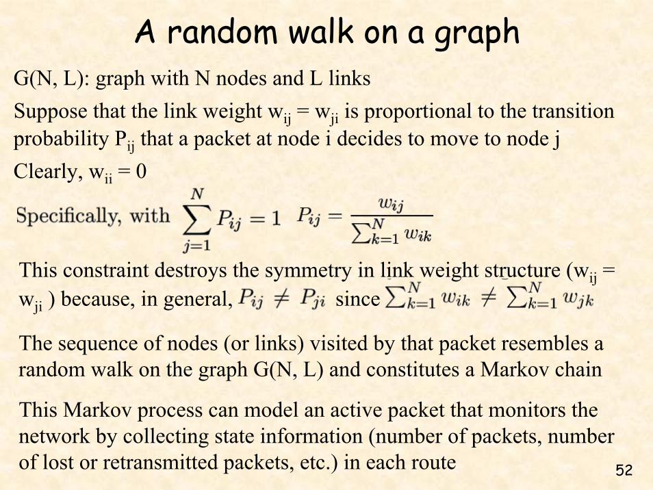
A random walk on a graphG(N, L): graph with N nodes and L linksSuppose that the link weight wij = wji is proportional to the transition probability Pij that a packet at node i decides to move to node j Clearly, wii = 0

This constraint destroys the symmetry in link weight structure (wij = wji ) because, in general, since

The sequence of nodes (or links) visited by that packet resembles a random walk on the graph G(N, L) and constitutes a Markov chain

This Markov process can model an active packet that monitors thenetwork by collecting state information (number of packets, number of lost or retransmitted packets, etc.) in each route

5353

A random walk on a graph

The condition for time reversibility becomes

The steady-state of this Markov process is readily obtained by observing that the chain is time reversible

For the collection of these data, the active packet should in steady-statevisit all nodes about equally frequently or πi = 1/N, implying that theMarkov transition matrix P must be doubly stochastic

5454

Slotted AlohaN nodes that communicate via a shared channel using slotted AlohaTime is slotted, packets are of the same sizeA node transmits a newly arrived packet in the next timeslotIf two nodes transmit at the same timeslot (collision) packets must be retransmittedBacklogged nodes (nodes with packets to be retransmitted) wait forsome random number of timeslots before retransmittingPacket arrivals at a node form a Poisson process with mean rate λ/N, where λ is the overall arrival rate at the network of N nodes

We ignore queuing of packets at a node (newly arrived packets are discarded if there is a packet to be retransmitted)We assume, for simplicity, that pr is the probability that a noderetransmits in the next time slot

5555

Slotted AlohaSlotted Aloha constitutes a DTMC with Xke{0, 1 ,2 ,… }, where

•state j counts the number of backlogged nodes •k refers to the k-th timeslot

Each of the j backlogged nodes retransmits a packet in the next time slot with probability pr

Each of the N-j unbacklogged nodes transmits a packet in the next time slot iff a packet arrives in the current timeslot which occurs with probability

For Poissonean arrival processThe probability that n backlogged nodes in state j retransmit in thenext time slot is binomially distributed

5656

Slotted AlohaSimilarly, the probability that n unbacklogged nodes in state j transmitin the next time slot is

A packet is transmitted successfully iff(a)one new arrival and no backlogged packet or(b)no new arrival and one backlogged packet is transmitted

The probability of successful transmission in state j and per slot is

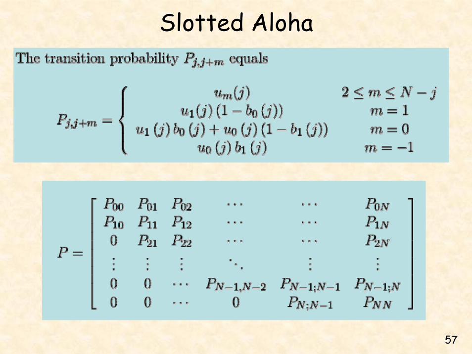
5757

Slotted Aloha

5858

State j (j backlogged nodes) jumps to•state j-1 if there are no new packets and one retransmission•state j if

•there is 1 new arrival and there are no retransmissions or•there are no new arrivals and none or more than 1 retransmissions

•state j+1 if there is 1 new arrival from a non-backlogged node and atleast 1 retransmission (then there are surely collisions)•state j + m if m new packets arrive from m different non-backloggednodes, which always causes collisions for m>1

Slotted Aloha

5959

Slotted Aloha

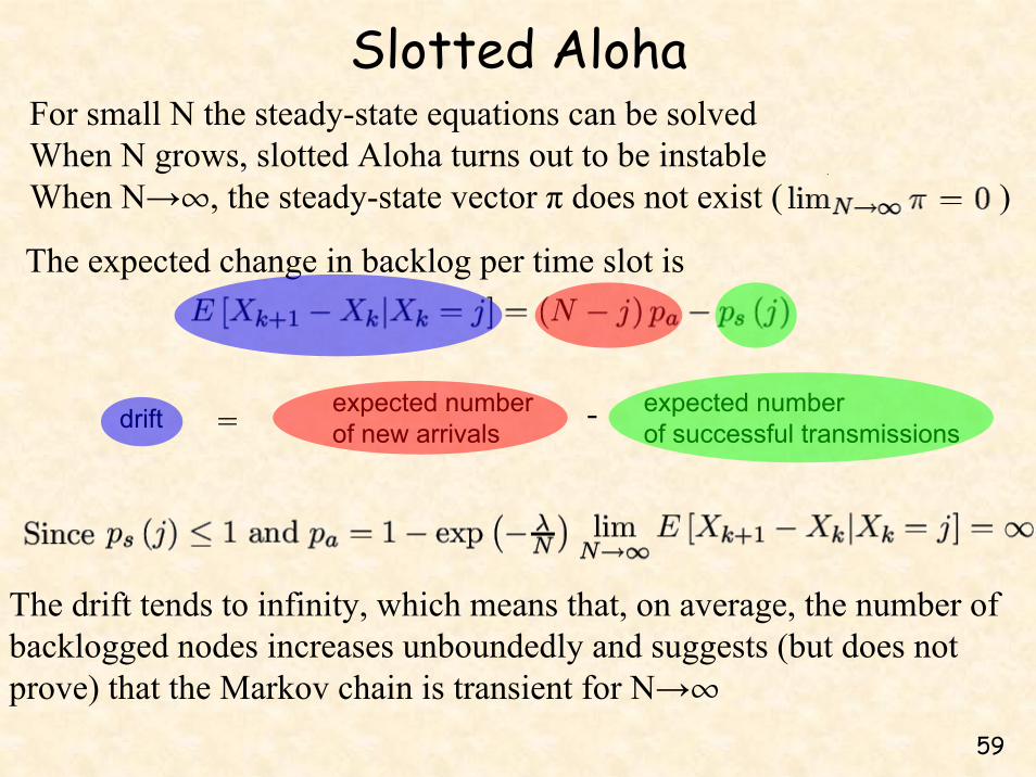
Τhe drift tends to infinity, which means that, on average, the number ofbacklogged nodes increases unboundedly and suggests (but does notprove) that the Markov chain is transient for N→¶

The expected change in backlog per time slot is

For small N the steady-state equations can be solvedWhen N grows, slotted Aloha turns out to be instableWhen N→¶, the steady-state vector π does not exist ( )

expected numberof new arrivals

expected numberof successful transmissionsdrift = -

6060

Efficiency of slotted Aloha

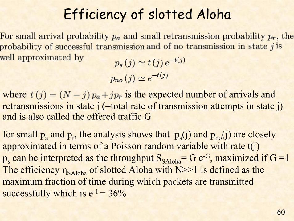
where is the expected number of arrivals and retransmissions in state j (=total rate of transmission attempts in state j)and is also called the offered traffic G

for small pa and pr, the analysis shows that ps(j) and pno(j) are closely approximated in terms of a Poisson random variable with rate t(j) ps can be interpreted as the throughput SSAloha= G e-G, maximized if G =1 The efficiency ηSAloha of slotted Aloha with N>>1 is defined as the maximum fraction of time during which packets are transmitted successfully which is e-1 = 36%

6161

Pure Aloha: the nodes can start transmitting at arbitrary times Performs half as efficiently as slotted Aloha with ηPAloha = 18%A transmitted packet at t is successful if no other is sent in (t-1, t+1) which is equal to two timeslots and thus ηPAloha = 1/2 ηSAloha

Ιn pure Aloha, because in (t-1, t+1) the expectednumber of arrivals and retransmissions is twice that in slotted Aloha

The throughput S roughly equals the total rate of transmissionattempts G (which is the same as in slotted Aloha) multiplied by

Efficiency of pure Aloha

6262

Ranking of webpagesWebsearch engines apply a ranking criterion to sort the list of pagesrelated to a queryPageRank (the hyperlink-based ranking system used by Google) exploits the power of discrete Markov theoryMarkov model of the web: directed graph with N nodes

•Each node in the webgraph represents a webpage and•the directed edges represent hyperlinks

6363

Ranking of webpagesAssumption:importance of a webpage ~ number of times that this page is visitedConsider a DTMC with transition probability matrix P that corresponds to the adjacency matrix of the webgraph

•Pij is the probability of moving from webpage i (state i) towebpage j (state j) in one time step•The component si[k] of the state vector s[k] denotes theprobability that at time k the webpage i is visited

The long run mean fraction of time that webpage i is visited equals the steady-state probability πi of the Markov chainThis probability πi is the ranking measure of the importance of webpage i used in Google

6464

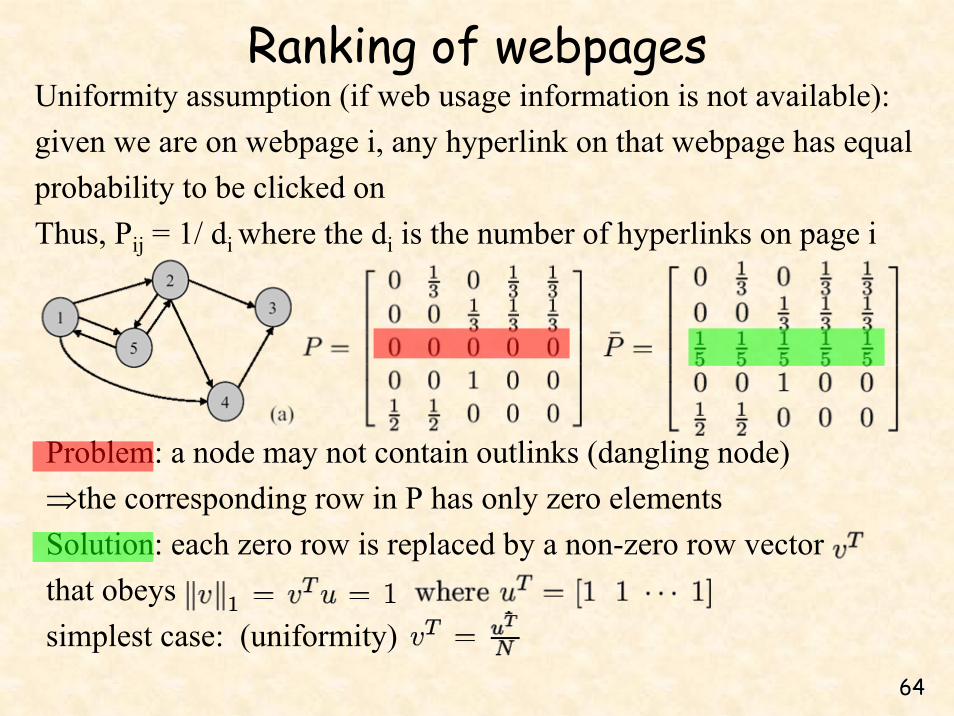
Ranking of webpagesUniformity assumption (if web usage information is not available): given we are on webpage i, any hyperlink on that webpage has equal probability to be clicked on Thus, Pij = 1/ di where the di is the number of hyperlinks on page i

Problem: a node may not contain outlinks (dangling node)⇒the corresponding row in P has only zero elementsSolution: each zero row is replaced by a non-zero row vectorthat obeys simplest case: (uniformity)

6565

Ranking of webpagesThe existence of a steady-state vector π must be ensuredIf the Markov chain is irreducible, the steady-state vector existsIn an irreducible Markov chain any state is reachable from any other By its very nature, the WWW leads almost surely to a reducible MC Brin and Page have proposed

where 0<a<1 and v is a probability vector (each component of v is non-zero in order to guarantee reacability)

6666

Computation of the PageRank steady-state vectorA more effective way to implement the described idea is to define a special vector r whose component rj = 1 if row j in P is a zero-row or node j is dangling nodeThen, is a rank-one update of and so is because

Specifically, for any starting vector s[0] (usually s[0] = ), weiterate the equation s[k+1]=s[k] P m-times and choose m sufficientlylarge such that where is a prescribed tolerance

Brin and Page propose to compute the steady-state vector from

6767

Computation of the PageRank steady-state vectorIt holds

Thus, only the product of s[k] with the (extremely) sparse matrix P needsto be computed and and are never formed nor storedPPFor any personalization vector, the second largest eigenvalue of is αλ2, where λ2 is the second largest eigenvalue of

PP

*

Brin and Page report that only 50 to 100 iterations of * for α= 0.85 are sufficientA fast convergence is found for small α, but then the characteristics of the webgraph are suppressed

Langville and Meyer proposed to introduce one dummy node that isconnected to all other nodes and to which all other nodes are connectedto ensure overall reachability. Such approach changes the webgraph less