Computational methods for continuous time Markov chains with applications to biological processes David F. Anderson * * [email protected]Department of Mathematics University of Wisconsin - Madison Penn. State January 13th, 2012
Transcript
Computational methods for continuous time Markov chainswith applications to biological processes
1David F. Anderson and Desmond J. Higham, Multi-level Monte Carlo for stochastically modeledchemical kinetic systems. To appear in SIAM: Modeling and Simulation. Available atarxiv.org:1107.2181. Also at www.math.wisc.edu/˜anderson.
1David F. Anderson and Desmond J. Higham, Multi-level Monte Carlo for stochastically modeledchemical kinetic systems. To appear in SIAM: Modeling and Simulation. Available atarxiv.org:1107.2181. Also at www.math.wisc.edu/˜anderson.
1. Weak error plays no role in analysis: free to choose hL.
2. Common problems associated with tau-leaping
I Negativity of species numbers,
does not matter. Just define process in a sensible way.
3. The method is unbiased.
Multi-level Monte Carlo: an unbiased estimator
Some observations:
1. Weak error plays no role in analysis: free to choose hL.
2. Common problems associated with tau-leaping
I Negativity of species numbers,
does not matter. Just define process in a sensible way.
3. The method is unbiased.
Multi-level Monte Carlo: an unbiased estimator
Some observations:
1. Weak error plays no role in analysis: free to choose hL.
2. Common problems associated with tau-leaping
I Negativity of species numbers,
does not matter. Just define process in a sensible way.
3. The method is unbiased.
Example
Consider a model of gene transcription and translation:
G 25→ G + M,
M 1000→ M + P,
P + P 0.001→ D,
M 0.1→ ∅,
P 1→ ∅.
Suppose:
1. initialize with: G = 1, M = 0, P = 0, D = 0,
2. want to estimate the expected number of dimers at time T = 1,
3. to an accuracy of ± 1.0 with 95% confidence.
ExampleMethod: Exact algorithm with crude Monte Carlo.
Approximation # paths CPU Time # updates3,714.2 ± 1.0 4,740,000 149,000 CPU S (41 hours!) 8.27 ×10¹⁰
Method: Euler tau-leaping with crude Monte Carlo.
Step-size Approximation # paths CPU Time # updatesh = 3−7 3,712.3 ± 1.0 4,750,000 13,374.6 S 6.2× 10¹⁰
h = 3−6 3,707.5 ± 1.0 4,750,000 6,207.9 S 2.1× 10¹⁰
h = 3−5 3,693.4 ± 1.0 4,700,000 2,803.9 S 6.9× 10⁹
h = 3−4 3,654.6 ± 1.0 4,650,000 1,219.0 S 2.6× 10⁹
Method: unbiased MLMC with `0 = 2, and M and L detailed below.Step-size parameters Approx. CPU Time # updates
M = 3, L = 6 3,713.9 ± 1.0 1,063.3 S 1.1 ×10⁹
M = 3, L = 5 3,714.7 ± 1.0 1,114.9 S 9.4 ×10⁸
M = 3, L = 4 3,714.2 ± 1.0 1,656.6 S 1.0 ×10⁹
M = 4, L = 4 3714.2 ± 1.0 1,334.8 S 1.1 ×10⁹
M = 4, L = 5 3,713.8 ± 1.0 1,014.9 S 1.1 ×10⁹
I the exact algorithm with crude Monte Carlo demanded 140 times moreCPU time than our unbiased MLMC estimator!
Example
Method: Exact algorithm with crude Monte Carlo.
Approximation # paths CPU Time # updates3,714.2 ± 1.0 4,740,000 149,000 CPU S (41 hours!) 8.27 ×10¹⁰
Unbiased Multi-level Monte Carlo with M = 3, L = 5, and `0 = 2.
Level # paths CPU Time Var. estimator # updates(X ,Z3−5) 3,900 279.6 S 0.0658 6.8 ×10⁷
(Z3−5 ,Z3−4) 30,000 49.0 S 0.0217 8.8 ×10⁷
(Z3−4 ,Z3−3) 150,000 71.7 S 0.0179 1.5 ×10⁸
(Z3−3 ,Z3−2) 510,000 112.3 S 0.0319 1.7 ×10⁸
Tau-leap with h = 3−2 8,630,000 518.4 S 0.1192 4.7 ×10⁸
Totals N.A. 1031.0 S 0.2565 9.5 ×10⁸
Some conclusions about this method1. Gillespie’s algorithm is by far the most common way to compute
expectations:
1.1 Means.
1.2 Variances.
1.3 Probabilities.
2. The new method (MLMC) also performs this task with no bias (exact).
3. Will be at worst the same speed as Gillespie(exact algorithm + crude Monte Carlo).
4. Will commonly be many orders of magnitude faster.
5. Applicable to essentially all continuous time Markov chains:
X (t) = X (0) +∑
k
Yk
(∫ t
0λk (X (s))ds
)ζk .
6. Con: Is substantially harder to implement; good software is needed.
7. Makes no use of any specific structure or scaling in the problem.
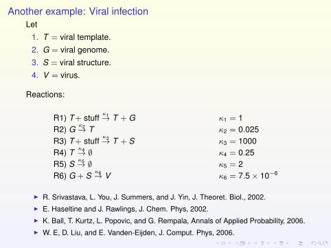
Another example: Viral infectionLet
1. T = viral template.
2. G = viral genome.
3. S = viral structure.
4. V = virus.
Reactions:
R1) T+ stuffκ1→ T + G κ1 = 1
R2) Gκ2→ T κ2 = 0.025
R3) T+ stuffκ3→ T + S κ3 = 1000
R4) Tκ4→ ∅ κ4 = 0.25
R5) Sκ5→ ∅ κ5 = 2
R6) G + Sκ6→ V κ6 = 7.5× 10⁻⁶
I R. Srivastava, L. You, J. Summers, and J. Yin, J. Theoret. Biol., 2002.I E. Haseltine and J. Rawlings, J. Chem. Phys, 2002.I K. Ball, T. Kurtz, L. Popovic, and G. Rempala, Annals of Applied Probability, 2006.I W. E, D. Liu, and E. Vanden-Eijden, J. Comput. Phys, 2006.
Another example: Viral infection
Stochastic equations for X = (XG,XS ,XT ,XV ) are
X1(t) = X1(0) + Y1
(∫ t
0X3(s)ds
)− Y2
(0.025
∫ t
0X1(s)ds
)− Y6
(7.5× 10⁻⁶
∫ t
0X1(s)X2(s)ds
)X2(t) = X2(0) + Y3
(1000
∫ t
0X3(s)ds
)− Y5
(2∫ t
0X2(s)ds
)− Y6
(7.5× 10⁻⁶
∫ t
0X1(s)X2(s)ds
)X3(t) = X3(0) + Y2
(0.025
∫ t
0X1(s)ds
)− Y4
(0.25
∫ t
0X3(s)ds
)X4(t) = X4(0) + Y6
(7.5× 10⁻⁶
∫ t
0X1(s)X2(s)ds
).
Another example: Viral infection
Reactions:
R1) T+ stuffκ1→ T + G κ1 = 1
R2) Gκ2→ T κ2 = 0.025
R3) T+ stuffκ3→ T + S κ3 = 1000
R4) Tκ4→ ∅ κ4 = 0.25
R5) Sκ5→ ∅ κ5 = 2
R6) G + Sκ6→ V κ6 = 7.5× 10⁻⁶
If T > 0,I reactions 3 and 5 are much faster than others.I Looks like S is approximately Poisson(500× T ).
Can average out to get approximate process Z (t).
Another example: Viral infection
Approximate process satisfies.
Z1(t) = X1(0) + Y1
(∫ t
0Z3(s)ds
)− Y2
(0.025
∫ t
0Z1(s)ds
)− Y6
(3.75× 10⁻³
∫ t
0Z1(s)Z3(s)ds
)Z3(t) = X3(0) + Y2
(0.025
∫ t
0Z1(s)ds
)− Y4
(0.25
∫ t
0Z3(s)ds
)Z4(t) = X4(0) + Y6
(3.75× 10⁻³
∫ t
0Z1(s)Z3(s)ds
).
(1)
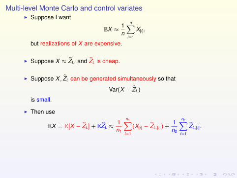
Now useEf (X (t)) = E[f (X (t))− f (Z (t))] + Ef (Z (t)).
Another example: Viral infection
X(t) = X(0) + Y1,1
(∫ t
0min{X3(s), Z3(s)}ds
)ζ1 + Y1,2
(∫ t
0X3(s)− min{X3(s), Z3(s)}ds
)ζ1
+ Y2,1
(0.025
∫ t
0min{X1(s), Z1(s)}ds
)ζ2 + Y2,2
(0.025
∫ t
0X1(s)− min{X1(s), Z1(s)}ds
)ζ2
+ Y3
(1000
∫ t
0X3(s)ds
)ζ3
+ Y4,1
(0.25
∫ t
0min{X3(s), Z3(s)}(s)ds
)ζ4 + Y4,2
(0.25
∫ t
0X3(s)− min{X3(s), Z3(s)}(s)ds
)ζ4
+ Y5
(2∫ t
0X2(s)ds
)ζ5
+ Y6,1
(∫ t
0min{λ6(X(s)), Λ6(Z (s))}ds
)ζ6 − Y6,2
(∫ t
0λ6(X(s))− min{λ6(X(s)), Λ6(Z (s))}ds
)ζ6
Z (t) = Y1,1
(∫ t
0min{X3(s), Z3(s)}ds
)ζ1 + Y1,3
(∫ t
0Z3(s)− min{X3(s), Z3(s)}ds
)ζ1
+ Y2,1
(0.025
∫ t
0min{X1(s), Z1(s)}ds
)ζ2 + Y2,3
(0.025
∫ t
0Z1(s)− min{X1(s), Z1(s)}ds
)ζ2
+ Y4,1
(0.25
∫ t
0min{X3(s), Z3(s)}(s)ds
)ζ4 + Y4,3
(0.25
∫ t
0Z3(s)− min{X3(s), Z3(s)}(s)ds
)ζ4
+ Y6,1
(∫ t
0min{λ6(X(s)), Λ6(Z (s))}ds
)ζ6 − Y6,3
(∫ t
0Λ6(Z (s))− min{λ6(X(s)), Λ6(Z (s))}ds
)ζ6,
Another example: Viral infection
Suppose wantEXvirus(20)
Given T (0) = 10, all others zero.
Method: Exact algorithm with crude Monte Carlo.
Approximation # paths CPU Time # updates13.85 ± 0.07 75,000 24,800 CPU S 1.45× 10¹⁰
Method: Ef (X (t)) = E[f (X (t))− f (Z (t))] + Ef (Z (t)).
Approximation CPU Time # updates13.91 ± 0.07 1,118.5 CPU S 2.41× 10⁸
Exact + crude Monte Carlo used:
1. 60 times more total steps.
2. 22 times more CPU time.
Mathematical Analysis
We had
X (t) = X (0) +∑
k
Yk
(∫ t
0λ′k (X (s))ds
)ζk .
Assumed ∑k
λ′k (X (·)) ≈ N � 1.
There are therefore two extreme parameters floating around our models:
1. Some parameter N � 1, causing N � 1 (inherent to model).
2. h, the stepsize (inherent to approximation).
To quantify errors, need to account for both.
Mathematical Analysis: Scaling in style of Thomas Kurtz
For each species i , define the normalized abundance
X Ni (t) = N−αi Xi(t),
where αi ≥ 0 should be selected so that X Ni = O(1).
Rate constants, κ′k , may also vary over several orders of magnitude. We write
κ′k = κk Nβk
where the βk are selected so that κk = O(1).
Eventually leads to scaled model
X N(t) = X N(0) +∑
k
Yk
(Nγ
∫ t
0Nβk +α·νk−γλk (X N(s))ds
)ζN
k .
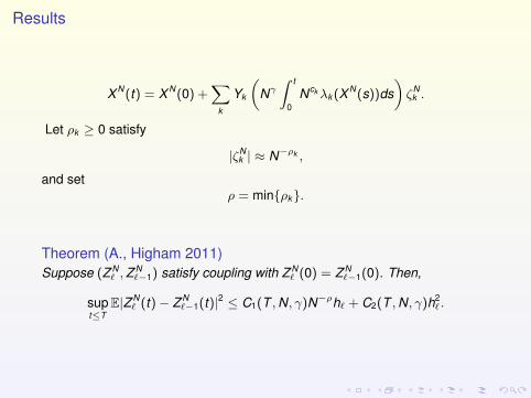
Results
X N(t) = X N(0) +∑
k
Yk
(Nγ
∫ t
0Nckλk (X N(s))ds
)ζN
k .
Let ρk ≥ 0 satisfy
|ζNk | ≈ N−ρk ,
and setρ = min{ρk}.
Theorem (A., Higham 2011)Suppose (Z N
` ,ZN`−1) satisfy coupling with Z N
` (0) = Z N`−1(0). Then,
supt≤T
E|Z N` (t)− Z N
`−1(t)|2 ≤ C1(T ,N, γ)N−ρh` + C2(T ,N, γ)h2` .
Results
X N(t) = X N(0) +∑
k
Yk
(Nγ
∫ t
0Nckλk (X N(s))ds
)ζN
k .
Let ρk ≥ 0 satisfy
|ζNk | ≈ N−ρk ,
and setρ = min{ρk}.
Theorem (A., Higham 2011)Suppose (X N ,Z N
` ) satisfy coupling with X N(0) = Z N` (0). Then,
There are multiple methods. We consider finite differences:
J ′(θ) =J(θ + ε)− J(θ)
ε+ O(ε).
Next problem: parameter sensitivities.
Motivated by Jim Rawlings.
We have
X θ(t) = X θ(0) +∑
k
Yk
(∫ t
0λθk (X
θ(s))ds)ζk .
and we define
J(θ) = Ef (X θ(t)].
We wantJ ′(θ) =
ddθ
Ef (X θ(t)).
There are multiple methods. We consider finite differences:
J ′(θ) =J(θ + ε)− J(θ)
ε+ O(ε).
Next problem: parameter sensitivities.
Motivated by Jim Rawlings.
We have
X θ(t) = X θ(0) +∑
k
Yk
(∫ t
0λθk (X
θ(s))ds)ζk .
and we define
J(θ) = Ef (X θ(t)].
We wantJ ′(θ) =
ddθ
Ef (X θ(t)).
There are multiple methods. We consider finite differences:
J ′(θ) =J(θ + ε)− J(θ)
ε+ O(ε).
Next problem: parameter sensitivities.
Motivated by Jim Rawlings.
We have
X θ(t) = X θ(0) +∑
k
Yk
(∫ t
0λθk (X
θ(s))ds)ζk .
and we define
J(θ) = Ef (X θ(t)].
We wantJ ′(θ) =
ddθ
Ef (X θ(t)).
There are multiple methods. We consider finite differences:
J ′(θ) =J(θ + ε)− J(θ)
ε+ O(ε).
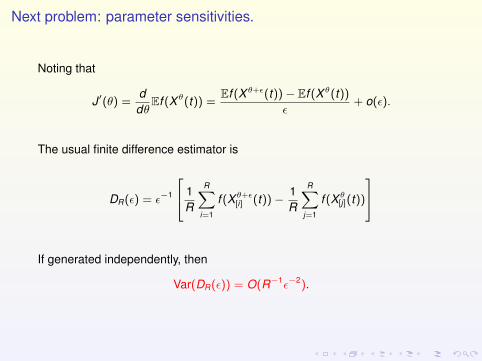
Next problem: parameter sensitivities.
Noting that
J ′(θ) =ddθ
Ef (X θ(t)) =Ef (X θ+ε(t))− Ef (X θ(t))
ε+ o(ε).
The usual finite difference estimator is
DR(ε) = ε−1
1R
R∑i=1
f (X θ+ε[i] (t))− 1
R
R∑j=1
f (X θ[j](t))
If generated independently, then
Var(DR(ε)) = O(R−1ε−2).
Next problem: parameter sensitivities.
Noting that
J ′(θ) =ddθ
Ef (X θ(t)) =Ef (X θ+ε(t))− Ef (X θ(t))
ε+ o(ε).
The usual finite difference estimator is
DR(ε) = ε−1
1R
R∑i=1
f (X θ+ε[i] (t))− 1
R
R∑j=1
f (X θ[j](t))
If generated independently, then
Var(DR(ε)) = O(R−1ε−2).
Next problem: parameter sensitivities.
Couple the processes.
X θ+ε(t) = X θ+ε(0) +∑
k
Yk,1
(∫ t
0λθ+ε
k (X θ+ε(s)) ∧ λθk (X θ(s))ds)ζk
+∑
k
Yk,2
(∫ t
0λθ+ε
k (X θ+ε(s))− λθ+εk (X θ+ε(s)) ∧ λθk (X θ(s))ds
)ζk
X θ(t) = X θ(0) +∑
k
Yk,1
(∫ t
0λθ+ε
k (X θ+ε(s)) ∧ λθk (X θ(s))ds)ζk
+∑
k
Yk,3
(∫ t
0λθk (X
θ(s))− λθ+εk (X θ+ε(s)) ∧ λθk (X θ(s))ds
)ζk ,
Use:
DR(ε) = ε−1 1R
R∑i=1
[f (X θ+ε
[i] (t))− f (X θ[i](t))
].
Next problem: parameter sensitivities.
Theorem (Anderson, 2011)Suppose (X θ+ε,X θ) satisfy coupling. Then, for any T > 0 there is a CT ,f > 0for which
E
[supt≤T
(f (X θ+ε(t))− f (X θ(t))
)2]≤ CT ,f ε.
This lowers variance of estimator from
O(R−1ε−2),
toO(R−1ε−1).
Lowered by order of magnitude (in ε).
1David F. Anderson, An efficient Finite Difference Method for Parameter Sensitivities ofContinuous Time Markov Chains. Submitted. Available at arxiv.org:1109.2890. Also atwww.math.wisc.edu/˜anderson.
TheoremSuppose (X θ+ε,X θ) satisfy coupling. Then, for any T > 0 there is a CT ,f > 0for which
E supt≤T
(f (X θ+ε(t))− f (X θ(t))
)2≤ CT ,f ε.
Proof:
Key observation of proof:
X θ+ε(t)− X θ(t) = Mθ,ε(t) +∫ t
0F θ+ε(X θ+ε(s))− F θ(X θ(s))ds.
Now work on Martingale and absolutely continuous part.
Analysis
TheoremSuppose (X θ+ε,X θ) satisfy coupling. Then, for any T > 0 there is a CT ,f > 0for which
E supt≤T
(f (X θ+ε(t))− f (X θ(t))
)2≤ CT ,f ε.
Proof:Key observation of proof:
X θ+ε(t)− X θ(t) = Mθ,ε(t) +∫ t
0F θ+ε(X θ+ε(s))− F θ(X θ(s))ds.
Now work on Martingale and absolutely continuous part.
Thanks!
References:
1. David F. Anderson and Desmond J. Higham, Multi-level Monte Carlo forcontinuous time Markov chains, with applications in biochemical kinetics,to appear in SIAM: Multiscale Modeling and Simulation.
Available at arXiv.org:1107.2181. Also on my website:www.math.wisc.edu/˜anderson.
2. David F. Anderson, Efficient Finite Difference Method for ParameterSensitivities of Continuous time Markov Chains, submitted.
Available at arXiv.org:1109.2890. Also on my website:www.math.wisc.edu/˜anderson.