Enhanced decentralized PI control for fluidized bed combustor viaadvanced disturbance observer

Li Sun a,n, Donghai Li a, Kwang Y. Lee b

a The State Key Lab of Power Systems, Department of Thermal Engineering, Tsinghua University, Beijing 100084, PR Chinab Department of Electrical and Computer Engineering, Baylor University, Waco, TX 76798-7356, USA

a r t i c l e i n f o

Article history:Received 22 January 2015Accepted 28 May 2015Available online 25 June 2015

Keywords:Fluidized bed combustorBoilerPI controlDisturbance observerPower plant

a b s t r a c t

Motivation of this paper is to propose an engineering friendly control strategy to handle the variousdifficulties in fluidized bed combustor (FBC). The control objectives of FBC and the difficulties arisenfrom nonlinear dynamics, frequent disturbances and strong coupling are first formulated. The capabilityof the disturbance observer (DOB) to handle the nonlinearity and disturbances is analyzed and thedecoupling effect of DOB is revealed in terms of equivalent transfer function. For the power loop, a robustloop shaping design method is proposed to balance the performance and robustness of DOB. For thetemperature loop, the DOB filter is designed based on H1 optimization. Abilities of DOB are confirmed bynumerical simulations. A water tank experiment is designed to show the simplicity of implementingDOB in an industrial Distributed Control System. Finally, a global simulation on the FBC processdemonstrates that, compared with the conventional PI scheme, the DOB-enhanced PI strategy achievesoverall improvement and can even be comparable with the complex Model Predictive Control in someaspects.

& 2015 Elsevier Ltd. All rights reserved.

1. Introduction

Fluidized bed combustor (FBC) boilers have been developedincreasingly in recent decades as an advanced clean coal technol-ogy (Ozdemir, Hepbasli, & Eskin, 2010). It facilitates burning of awide variety of fuels with high combustion efficiency, especiallyfor low-grade coal. The FBC was developed to strive for acombustion condition, under which the pollutant emissions canbe reduced significantly without a chemical scrubber. The burningtemperature of such technology is within the range of 750–950 1C,exactly out of the range where nitrogen oxides form so that theamount of NOx emission is just 1/3–1/4 of that in a conventionalpulverized coal plant. Thus, bed temperature regulation, alongwith strong capacity of load tracking, is critical to reduce pollutantemissions.

However, essentially, the FBC can be described as a typicalmultivariable system with almost all the difficulties found inprocess control, i.e., nonlinearities, strong couplings, various inter-nal and external disturbances, non-minimum phase (NMP), andtime delay. These difficulties result in enormous hardships oncontroller design. The conventional decentralized proportional-

integral (PI) control scheme is thus powerless in achievingsatisfactory performance under such extreme circumstances.Many researchers (Aygun, Demirel, & Cernat, 2012; Hadavand,Jalali, & Famouri, 2008; Leimbach, 2012; Ćojbašić, Nikolić, Ćirić, &Ćojbaši, 2011; Sun, Pan, & Shen, 2013; Zhang, Feng, Lu, & Xiang,2008) have worked on various advanced control schemes for FBCprocesses to accommodate some of the difficulties. Aygun andDemirel proposed a particle swarm optimization (PSO) algorithmto optimize the proportional-integral-derivative (PID) controllersfor the bed temperature (Aygun et al., 2012). An H1 controlalgorithm based on linear matrix inequalities (LMI) was alsoproposed in Hadavand et al., (2008) to improve the performanceof the bed temperature. However, strong interactions betweenpower and bed temperature were not considered. Intelligentcontrol strategies (Leimbach, 2012; Ćojbašić et al., 2011) were alsointroduced to facilitate the reference tracking of FBC boiler. But,there are few relevant literatures taking into an explicit considera-tion of the NMP characteristics in the FBC system. Model pre-dictive control (MPC), which is widely recognized as a powerfulstrategy in handling decoupling, reference tracking and timedelays, also received considerable attention in the FBC control(Sun et al., 2013; Zhang et al., 2008). However, the conventional orimproved MPCs are usually subject to a great deal of calculation,which makes it not feasible for the contemporary DistributedControl System (DCS) in power plant. Compared with the

Contents lists available at ScienceDirect

journal homepage: www.elsevier.com/locate/conengprac

Control Engineering Practice

http://dx.doi.org/10.1016/j.conengprac.2015.05.0140967-0661/& 2015 Elsevier Ltd. All rights reserved.

n Corresponding author.E-mail address: sunli12@mails.tsinghua.edu.cn (L. Sun).

Control Engineering Practice 42 (2015) 128–139

conventional PI controller, MPC usually requires an additionalcomputer, such as high-performance Programmable AutomationController (PAC), to calculate the control signals and then com-municate with DCS. Inevitably, it brings more hardware uncer-tainties into the system, which is unacceptable for practitionersbecause they always consider the long-term reliability as theirprimary concern.

The long-term running of FBC boiler is also subject to variousdisturbances, such as variations in the calorific value of feed coal,changing moisture content of the primary air, and slagging orerosion on the water wall. These disturbances, together with plantperturbations under different working conditions, deteriorate theperformance of the FBC process. Although previous researchesmainly focused on the reference tracking issue, they paid littleattention to the disturbance rejection.

As is well known, the basic PID controller, actually in mostcases PI controller, is still dominant in power generation for itssimplicity and ease of use (Xue, Li, & Gao, 2010). This paperattempts to accommodate all the aforementioned control difficul-ties within the framework of conventional decentralized PIscheme with the assistance of the disturbance observer (DOB)(Umeno & Hori, 1991). While PI controllers are responsible for thezero-offset reference tracking, the other control difficulties areexpected to be handled by the DOB, whose enhancement role isembodied as:

� The quasi feed-forward compensator which can estimate thedisturbances and then reject it actively;

� The plant re-shaper which can recover the nonlinear plant asthe nominal linear model in the wide operating range;

� The dynamic decoupler which requires lower modeling accu-racy than conventional methods.

With the advantages above, the DOB approaches have beenwidely utilized in many practical applications (see Chen, Yang, Li,and Li (2009), Li, Qiu, Ji, Zhu, and Li (2011), Liu Chen, and Andrews(2012) and references therein). In a traditional explanation of theDOB's decoupling ability, interaction is assumed as a part of thetotal disturbance, which should be observed by DOB and thenrejected. This paper will clarify the decoupling ability by bridgingDOB to the well-known inverted decoupling structure.

Considering the slow dynamics, time delay and NMP feature ofthe FBC boiler, the standard DOB is modified to achieve animproved performance. A water tank experiment is carried outto test the realizability of the proposed strategy in the DCS.

The feature that makes the proposed method distinct fromother advanced algorithms is attributed to the engineering friend-liness. The proposed strategy needs negligible amount of compu-tation and is completely compatible with already existing controlsystems. The DOB can be embedded into the DCS in a bumplessmanner without the necessity of retuning the PI parameters. Theremainder of the paper is organized as follows: the controldifficulties in the FBC system are formulated in Section 2.Section 3 analyzes the capability of DOB in dealing with thedisturbances, nonlinearity and coupling as well as the time delayand NMP characteristics. In Section 4, a numerical simulation andexperimental test is given to confirm the effectiveness andimplementability of DOB. A comparative simulation of the FBCapplication is carried out in Section 5 and conclusions are drawn inSection 6.

2. Problem formulation

2.1. Overview of fluidized Bed combustion technology

Fluidized bed suspends coal particles on continuous updraft ofprimary air during the combustion process, which leads to anintensive mixing of solid fuel and gas. The turbulent condition,similar to a bubbling fluid, leads to a higher efficiency for thechemical reactions and heat transfer. The schematic of a FBC boileris shown in Fig. 1. A mixture of inert/sorbent bed material andsolid fuel is fluidized by the primary air entering from below.Secondary air is injected above the fuel bed to ensure complete gasburning out. However the total amount of air should be limiteddue to economic efficiency. The heat released in combustion iscaptured by heat exchangers to convert the circulating water tothe steam.

2.2. Control objectives

The past two decades has witnessed a rapid development ofthe renewable energy generation. However the intermittent char-acteristics of the sustainable source make it more challenging tomaintain power grid stability. The conventional fossil fuel genera-tion should thus bear more responsibility in the primary frequencyregulation of power grid. In light of this background, the controlobjectives of FBC boiler is listed below in a descending order ofimportance:

I. The thermal power output of the boiler should track thereference load commanded by the turbine.

II. The bed temperature should be adjusted correspondingly to areasonable value.

III. The power output and the bed temperature should be asinsensitive as possible to the furnace disturbances.

The first requirement is set for the real-time balance of thepower grid or microgrid and the second for the environmental andeconomic purposes. Although the temperature range between750 1C and 950 1C can prevent the formation of NOx, a particularvalue is usually preferred for the combustion efficiency. Now thethird requirement is attracting considerable attention in engineer-ing practice but less from the academic community. Withoutproper treatment, the variation of the coal quality, i.e., the heatvalue perturbation, may make the boiler outputs deviate from thedesired value significantly.

Preheater

Superheater

Economizer

Coal feeder

1u

Mill

Secondaryair fan

bP

Primaryair fan

2u

CoalParticle

GasBubble

ToTurbine

Bed

Freeboard

SteamPower

Conveyerbelt

Fig. 1. A schematic of a typical fluidized bed combustor.

L. Sun et al. / Control Engineering Practice 42 (2015) 128–139 129

2.3. Dynamic model of FBC boiler

Zhou, Flamant, and Gauthier (2004) set up an elaborate modelof FBC to describe the complex turbulent characteristics based onthe 2-D Navier–Stokes equations. However the equations areexpected to be solved by the numerical method of large eddysimulation (LES), whose computational complexity makes it inap-propriate for a control simulation platform. Due to the turbulentcharacteristics of the FBC furnace, the plug flow model is also notapplicable. Ikonen and Kortela (1994) proposed a simple dynamicbubbling FBC model by separating the whole furnace as twointerconnected regions, bed and freeboard. By assuming eachregion as a continuous stirred-tank reactor (CSTR), the balanceequations were built based on the first law of thermodynamics.This simple model was validated by a 30 MW pilot coal combustorin the region from 19 MW to 28 MW, covering the normaloperating range of the FBC boiler. To achieve a balance betweenfidelity and simplicity, the model was slightly modified as follows(Ikonen & Najim, 2001; Sun, Dong, Li, & Zhang, 2014):

Dynamics of fuel inventory, WC [kg]:

dWCðtÞdt

¼ ð1�VÞQCðtÞ�QBðtÞ ð1Þ

Dynamics of bed oxygen content CB [N m3/N m3]:

dCBðtÞdt

¼ 1VB

½C1F1ðtÞ�QBðtÞXC�CBðtÞF1ðtÞ� ð2Þ

Dynamics of freeboard oxygen content, CF [N m3/N m3]:

dCF ðtÞdðtÞ ¼ 1

VFCBðtÞF1ðtÞþC2F2�VQCðtÞXV �CF ðtÞ½F1ðtÞþF2�� � ð3Þ

Dynamics of bed temperature, TB [K]:

dTBðtÞdt

¼ 1CIWI

HCQBðtÞþc1F1ðtÞT1 �αBtABt ½TBðtÞ�TBt ��cFF1ðtÞTBðtÞ� �

ð4Þ

Dynamics of freeboard temperature, TF [K]:

dTF ðtÞdt

¼ 1CFVF

HVVQCðtÞ�αFtAFt ½TF ðtÞ�TFt �þcFF1ðtÞTBðtÞ�

þc2F2T2ðtÞþc1 F1ðtÞþF2½ �TF ðtÞ� ð5Þ

Dynamics of thermal power, P [MW]:

dPðtÞdt

¼ 1τmix

½PCðtÞ�PðtÞ� ð6Þ

where the combustion rate in bed, QB [kg/s], isQBðtÞ ¼WCðtÞCBðtÞ=ðtCC1Þ, and the combustion power, PC [MW], isPC(t)¼10�6[HCQB(t)þHVVQC(t)]. The parameter settings can befound in Appendix.

According to the control objectives, manipulated inputs aredetermined as fuel feed QC [kg/s] (denoted as u1) and primary airflow F1 [N m3/s] (denoted as u2). Controlled variables are accord-ingly determined as output power P [MW] (denoted as y1) and bedtemperature TB [K] (denoted as y2). Freeboard oxygen content, CF,which can be easily controlled by secondary air, is relativelyindependent. It is found that delay is negligible for air flow, but20 s delay is necessary for fuel transport. Hereby a standardnonlinear model for control can be derived from (1)–(6) as:

_x¼ f ðx;uÞy¼ hðxÞ

(ð7Þ

where, x¼ ½WC CB CF TB TF P�T , u¼ ½QCðt�20Þ F1�T , y¼ ½TB P�T .Some representative operating conditions are shown in Table 1.

2.4. Control difficulties

In this section, the difficulties for FBC control will be analyzedin detail. The first one obviously originates from the time delay inthe fuel feed loop which will strictly limit the closed-loopbandwidth (Åström & Hagglund, 2006).

To further illustrate the difficulties, the model (7) is linearizedaround operating condition ‘4’,

Y1ðsÞY2ðsÞ

" #¼

G11ðsÞ G12ðsÞG21ðsÞ G22ðsÞ

!U1ðsÞU2ðsÞ

" #ð8Þ

An obvious distinction caused by nonlinearity can be seen inthe step-input responses of the original and locally linearizedmodel, are shown in Fig. 2. The strong coupling is also evident. Thefuel feed (u1) can significantly affect the power and the tempera-ture simultaneously. Although the primary air (u2) only influencesthe static value of the temperature, it may help release the thermalstorage in the bed and result in a power peak. The action ofprimary air could raise the output power rapidly by releasing bedheat storage at the very start while causing no effects at the end.

To quantitatively measure the nonlinearity of the system andprovide guidance for reference setting, the gap metric for multi-variable system (Tan, Marquez, Chen, & Liu, 2005) is used, which isdefined as

vg ¼ supr0

δðLr0N; LÞ ð9Þ

where, L is the nominal linear model of the nonlinear system N,and Lr0Nis the linearization of N at an operating point r0. The gapmetric δ in (9) is defined as:

δðP1; P2Þ ¼ max f δ!ðP1; P2Þ; δ!ðP2; P1Þg ð10Þ

where δ!ðP1; P2Þ and δ

!ðP2; P1Þ are the directed gaps. When twolinear systems are represented by normalized coprime factoriza-tions as P1 ¼N1M

�11 and P2 ¼N2M

�12 , the directed gap δ

!ðP1; P2Þcan be computed by

δ!ðP1; P2Þ ¼ inf

Q AH1

M1

N1

" #�

M2

N2

" #Q

����������1

ð11Þ

It follows that the closer is the distance to 1, the stronger is thenonlinearity of the system. In this paper, the intermediate operat-ing condition ‘4’ is chosen as the nominal model for controllerdesign. Fig. 3 shows the gap metric between the nominal modeland linearized models at other operating conditions around it.Note that the nominal condition ‘4’ is in the center of the variedrange. It is obviously seen that the nonlinearity increases with thedistance deviating from the nominal model. The resulting worst-case gap metric vg is 0.91, which represents a quite strongnonlinearity of the FBC system.

The valley existing in Fig. 3 shows that the nonlinearitymeasure can be somewhat attenuated by increasing or decreasingthe fuel feed and primary air simultaneously. This intuitivephenomenon happens to agree with the reference settings of

Table 1Steady-state operating conditions.

Operating condition QC [kg/s] F1 [N m3/s] PC [MW] TB [K]

1 2.50 3.50 20.25 9672 2.72 3.56 22.04 10053 2.83 3.62 22.93 10224 3.01 3.69 24.31 10495 3.12 3.73 25.34 10706 3.25 3.77 26.33 10917 3.37 3.80 27.38 10128 3.43 3.82 27.81 1123

L. Sun et al. / Control Engineering Practice 42 (2015) 128–139130

temperature and power for optimal combustion efficiency. Sincethe nonlinearity measures of operating conditions below andabove ‘4’ are approximately symmetric, the simulation will becarried out from condition ‘4’–‘8’ gradually in Section 5.

In addition to time delay, nonlinearity and strong coupling,another difficulty is raised by the non-minimum phase (NMP)characteristics, which is shown visually via the inverse response ofthe bed temperature [see Fig. 2(b)]. A set of field data from a300 MW circulating fluidized bed boiler in north China alsoconfirms the inverse response of the bed temperature, shown inFig. 4. The theoretical difficulty of the NMP control is attributed toits additional phase lag (Zhao, Sun, Li, & Gao, 2014). However herea nice physical interpretation can be made. In the initial period ofthe step response of the primary air, the suddenly injected air willhelp blow out the pulverized coal stacked in the bed and thenburn out to release the heat, therefore, the bed temperatureincreases rapidly. However, since the storage is non-sustainable

and more heat is brought away by the air, the bed temperature willeventually decrease in the steady state.

3. Analysis and advanced design of disturbance observer

This section attempts to demonstrate the ability of disturbanceobserver to accommodate the difficulties discussed above.

3.1. Disturbance observer

The general disturbance observer (DOB) is presented in Fig. 5.Its capabilities in dealing with external disturbances, modelinguncertainties, time delay and NMP was analyzed detailed in (Sun,Li, & Lee, 2015). Signals c(s), u(s), y(s) and n(s) are the controlleroutput, the manipulated variable, the controlled variable and thesensor noise, respectively. The process is decomposed into a

0 2000 4000 6000 8000 1000024

25

26

27

28

Pow

er [M

W]

0 2000 4000 6000 8000 100001000

1050

1100

1150

Time (s)

Tem

pera

ture

[K]

0 2000 4000 6000 8000 1000024.3

24.4

24.5

24.6

24.7

Pow

er [M

W]

0 2000 4000 6000 8000 100001000

1020

1040

1060

Time (s)Te

mpe

ratu

re [K

]Fig. 2. Step-input responses of the nonlinear and a linearized model (Solid line in red: nonlinear model; dotted line in blue: linearized model). (a) Step in QC (u1) with themagnitude of 0.4 kg/s (b) step in F1 (u2) with the magnitude of 0.4 N m3/s. (For interpretation of the references to color in this figure legend, the reader is referred to the webversion of this article.)

2.53

3.5

3.5

3.6

3.7

3.8

3.90

0.25

0.50

0.75

1

1.25

Feedcoal [kg/s]

v g

Primary Air [Nm 3/s]

Fig. 3. Distance measure around the nominal model.

0 50 100 150 200 250 300 350 400 450 500834

835

836

837

838

839

840

841

Time (s)

Tem

pera

ture

o C

Fig. 4. Step response of the bed temperature.

L. Sun et al. / Control Engineering Practice 42 (2015) 128–139 131

minimum phase function, PmðsÞ, and a non-reversible function,PiðsÞ, which may contain time delay and NMP elements with unitygain. The linear transfer function ~PmðsÞ is the nominal model ofPmðsÞ. Here the process nonlinearity is treated as modelinguncertainty beyond ~PmðsÞ. The low-pass filter Q(s) with unity gainis used to ensure the properness of DOB.

In the model matching case, ~PmðsÞ ¼ PmðsÞ, the DOB is trans-parent to the outer controller (i.e., it does not affect the dynamicsfrom c(s) to y(s)). Based on Mayson's rule, the closed-loop transferfunction from the disturbance d to its estimation d̂ is derived as:

DðsÞ ¼ d̂ðsÞdðsÞ ¼

Q ðsÞPiðsÞ1�Q ðsÞPiðsÞþQ ðsÞPiðsÞ

¼ Q ðsÞPiðsÞ ð12Þ

Since Q ðsÞPiðsÞis of unity gain, the disturbance observer canprovide a reasonable estimation of the real disturbance.

For analysis on the modeling uncertainty, an equivalent form ofFig. 5 is derived in Fig. 6. The transfer function from c(s) to y(s) canbe easily calculated as:

GcyðsÞ ¼PmðsÞ ~PmðsÞ

ð1�αðsÞÞ ~PmðsÞþαðsÞPmðsÞPiðsÞ ð13Þ

where, the weighting factorαðsÞ ¼ Q ðsÞPiðsÞ determines the normal-ization performance of DOB. If 1�αðjwÞ

�� �� can be shaped to equal tozero in the frequency range of interest, the new equivalent plantGcyðsÞcan be recovered as the nominal model ~PmðsÞPiðsÞ.

3.2. Decoupling ability

In addition to the abilities above, the decoupling effect of DOBhas also been observed in many applications (Chen et al., 2009;Sun et al., 2015). It is, however, not clear that why, how and inwhat condition the decoupling ability exists. Here, the two-inputtwo-output (TITO) minimum phase process is taken as an exam-ple, as shown in Fig. 7(a). Both loops are compensated by adisturbance observer, where ~g11and ~g22 are the nominal modelsof g11 and g22, respectively.

As shown in Fig. 7(b), the output signal y1(s) is divided into twoparts y11(s) and y12(s), which are assumed to be sent to DOBseparately. It is interesting to see that the resulting u0

1�y11 loophappens to be an inner loop enhanced by DOB, whose transferfunction at low frequencies can be approximated as:

Gu01y11ðsÞ ¼ g11ðsÞ ~g11ðsÞ

Q1ðsÞ½g11ðsÞ� ~g11ðsÞ�þ ~g11ðsÞ� ~g11ðsÞ ð14Þ

The final equivalent block diagram is thus obtained in Fig. 7(c),which is identical to the classical dynamic decoupling method,namely inverted decoupling (Wade, 1997). If there are modeluncertainties in the process, the DOB-based approach will possessrobustness advantages because the diagonal elements of theprocess are normalized as the model and non-diagonal elementsare not required in the DOB scheme. Actually it is the poorrobustness that limits the implementation of inverted decouplingin industry (Garduno-Ramirez & Lee, 2005). In the presence oftime delay or NMP in the process, the decoupling ability of DOBwill degrade but still remains partly. The disturbance observer canat least work as a static decoupler because PiðsÞ is of unity gain.

3.3. The DOB design for time-delay processes

The conventional Q filter of DOB was usually chosen as below:

Q ðsÞ ¼ 1ð1þTsÞn ð15Þ

For motion control or other processes with fast dynamics, theorder n was tuned to obtain a proper observer and the timeconstant T was usually determined by a desired bandwidth.However for the fuel-thermal power loop (G11) with time-delayand slow dynamics, such a design may produce a quite sluggishresponse though the time constant is chosen sufficiently small.The reason is that, as shown in (12), the disturbance can only beobserved after the time delay and then the compensation has to gothrough the slow process. To this end, a lead–lag module isintroduced to accelerate the response of disturbance rejection byartificially creating an overshoot in disturbance estimation. That is,the Q filter is designed as:

Q ðsÞ ¼ 1þλTf sð1þTf sÞð1þT1sÞn

ð16Þ

Tuning of Tf is determined by the expected settling time of theovershoot. A larger λ may lead to a quicker response but it alsoresults in smaller robustness stability margin. For a given process,i.e., G11, tuning of λ is thus a loop-shaping problem and a trade-offbetween the performance and the robustness. Based on thestructure shown in Fig. 6, assuming PiðsÞ ¼ e� τs and PmðsÞ ¼ ~PmðsÞ,the open-loop transfer function of the DOB enhanced process is

GLðsÞ ¼Q ðsÞe� τs

1�Q ðsÞe� τs ð17Þ

The closed-loop robustness can be evaluated on GLðsÞ in termsof two popular robustness indices, i.e., sensitivity index Ms andcomplementary sensitivity index Mt, defined as follows:

Ms ¼ max1

1þGLðiwÞ

�������� for any w ð18Þ

Mt ¼ maxGLðiwÞ

1þGLðiwÞ

�������� for any w ð19Þ

As recommended in Åström and Hagglund (2006), the robust-ness constraints on the DOB loop are chosen as: Ms¼1.8 andMt¼1.4, which may be satisfied by shaping the Nyquist plot of GL

outside the contour of each robustness index. Under settling timechosen as Tf¼100, the largest λ can be determined as 1.3 bydrawing a cluster of the Nyquist plots, shown in Fig. 8.

3.4. H1 optimization for the NMP–DOB filter

For the NMP process, it is possible to obtain an analytic solutionto the optimal filter. Referring to Fig. 5, the non-minimum phasepart was constructed as a transfer function that has unity

Fig. 5. General structure of the disturbance observer.

( ) ( )Q s P s

c(s) u0(s)u0(s) yy((s)))y(s)( ) ( )P s P s

11 ( ) ( )Q s P s

˜

Fig. 6. Equivalent diagram of the DOB.

L. Sun et al. / Control Engineering Practice 42 (2015) 128–139132

magnitude and a right-half plane zero 1/a,

PiðsÞ ¼1�as1þas

ð20Þ

Based on (12), the estimation error of the disturbance isaccordingly calculated as:

eðsÞ ¼ ð1�Q ðsÞPiðsÞÞdðsÞ ð21Þ

As the right-half plane zero cannot be canceled by the filter,(21) implies that the estimation of disturbance should also endurean initial inverse response, which would inevitably deteriorate thedisturbance rejection performance. To balance the initial inverseresponse and the subsequent tracking speed, an H1 optimizationproblem is formulated

min j j ½1�Q ðsÞPiðsÞ�dðsÞj j1 ð22Þ

Fig. 7. Schematic of the equivalent transformation. (a) Conventional decentralized feedback based on DOB. (b) Decomposition of DOB in terms of outputs. (c) Equivalent formof inverted decoupling.

L. Sun et al. / Control Engineering Practice 42 (2015) 128–139 133

The minimization in (22) will suppress the inverse responsewhile pursuing a fast tracking ability. Prior to solving this problem,a fundamental theorem (Solomentsev, 2001) of complex variablesshould be introduced:

3.4.1. Maximum modulus principleAssume that F(s) is holomorphic within a connected open

subset complex domain D. If F(s) is not a constant, then |F(s)| takesits maximum value on the boundary of D.

The stability of the estimation error e(s) guarantees that it hasno poles in the open right-half plane (RHP) of the complexvariables, thus let a subset complex domain D equal the openRHP. Note also that Pi(s) has a zero 1/a, which is located at theinterior of D. assuming the disturbance is a step input, i.e.,dðsÞ ¼ 1=s, thus

j j eðsÞj j1 ¼ j j ½1�Q ðsÞPiðsÞ�dðsÞj j1

¼ supRes40

j ½1�Q ðsÞPiðsÞ�dðsÞjZ j ½1�Q ðsÞPiðsÞ�dðsÞj s ¼ 1=a ¼ j eðsÞj s ¼ 1=a

ð23ÞBy letting eðsÞ � a, it is possible to obtain the following unique

optimal solution:

QoptðsÞ ¼1�a=dðsÞ

PiðsÞ¼ 1þas ð24Þ

Note that the optimal QoptðsÞ is improper. A low-pass filter mustbe introduced to make the DOB implementable. Thus a sub-optimal filter can be obtained as:

Q ðsÞ ¼ 1þas

ð1þT2sÞ4ð25Þ

It is shown that the proposed filter has a zero, which isdifferent from the conventional form.

4. Disturbance rejection abilities and implementation in DCS

All the control difficulties in the FBC system are identified inSection 2, which are expected to be handled under the frameworkof the disturbance observer (DOB), as analyzed in Section 3. In thissection, simulations are carried out to demonstrate the abilitiespoint by point. At last, a water tank experiment is designed toshow the most important virtue of DOB: realizability in DCS.

4.1. Disturbance rejection

The disturbance observer in Section 3.3 is applied in thenominal linear model (G11) of the power loop of FBC. Assuminga step load disturbance is added at t¼1000 s, the performance ofdisturbance rejection is shown in Fig. 9. It can be found that theoutput can be dragged back faster to steady state with theimproved DOB.

The disturbance observer in Section 3.4 is applied in thenominal linear model (G22) of the temperature loop of FBC. Theimprovement is validated via a simulation by adding a stepdisturbance at t¼1000 s, as shown in Fig. 10. Compared with theconventional filter, the suboptimal design gives a faster conver-gence rate but with the same magnitude of inverse response andmore smooth control action. Note that there are no PI controllersin these two examples, and the disturbance is rejected onlyby DOB.

-3.5 -3 -2.5 -2 -1.5 -1 -0.5 0 0.5-2

-1.5

-1

-0.5

0

0.5

1

1.5

2

Real Axis

Imag

inar

y A

xis

=1

=1.8

=1.5 =1.3

M t =1.4

M s=1.8

λ

λ λ

λ

Fig. 8. The open-loop Nyquist plots of the time-delay processes with DOB.

0 500 1000 1500 2000 2500 3000 3500 4000 4500 50000

0.5

1

Time (s)

y

0 500 1000 1500 2000 2500 3000 3500 4000 4500 5000-1.5

-1

-0.5

0

Time (s)

u

Fig. 9. The performance of disturbance rejection in the time delay process (Bluesolid: λ¼1; red dashed: λ¼1.3). (For interpretation of the references to color in thisfigure legend, the reader is referred to the web version of this article.)

0 500 1000 1500 2000 2500 3000 3500 4000 4500 5000-100

-50

0

50

Time (s)

y

0 500 1000 1500 2000 2500 3000 3500 4000 4500 5000-1.5

-1

-0.5

0

0.5

Time (s)

u

Fig. 10. Disturbance rejection for step disturbance in the NMP process (Solid inblue: conventional filter; dashed in red: modified filter). (For interpretation of thereferences to color in this figure legend, the reader is referred to the web version ofthis article.)

L. Sun et al. / Control Engineering Practice 42 (2015) 128–139134

4.2. Performance recovery

The power loop of FBC is chosen to validate the performancerecovery ability of DOB. Step responses (from c to y in Fig. 5) underdifferent operating conditions are shown in Fig. 11. It is easy to seethat the step responses under the different working conditions areshaped almost the same due to the compensation effect of DOB.

4.3. Decoupling

A simple minimum phase TITO plant is constructed to clearlyshow the decoupling ability analyzed in Section 3.2,

GðsÞ ¼2

1þ5s1:5

1þ4s

" 1:21þ s3

1þ2s

#ð26Þ

The control system is configured in the form of Fig. 7(a). Each PIcontroller is tuned by the pole placement method (Åström &Hagglund, 2006). The simulation results for the decentralized PIwith and without DOB are shown in Fig. 12. Obviously, the DOB-PIscheme can obtain a very good decoupling performance.

4.4. An experimental realization in DCS

In this section, the realization of the DOB-enhanced PI strategyis tested in a water tank system, as shown in Fig. 13. The controlledvariable is the water level and the control input is the pump rotorspeed. The experimental results of PI controller without and withDOB compensation are shown in Fig. 14. Obviously, the DOB-PIcontrol system works very well and the resulting performance ismuch less sensitive to the operating condition compared with theconventional PI control system.

5. Application to the nonlinear FBC boiler

The abilities of DOB have been confirmed in the simple linearcases in Section 4. In this section, the simulation will be carried outby applying the DOB enhanced PI control strategy on the nonlinearFBC model, as shown in Fig. 15, where, G11mand G22mare theminimum parts of G11 and G22, respectively, and Giis the non-minimum phase part of G22.

The performance under the DOB-enhanced decentralized PIscheme will be compared with and without DOB compensation. Tofurther demonstrate that the proposed strategy can rival thecomplex MPC, a set of parameters of state space MPC were tuned.

0 1000 2000 3000 4000 5000 6000 70000

1

2

3

4

5

6

7

8

9

Time (seconds)

Am

plitu

de

0 2000 4000 6000 8000 10000 12000 14000 160000

1

2

3

4

5

6

7

8

9

Time (seconds)

Am

plitu

de

Fig. 11. The step responses of the linearized models with (Top) and without(Bottom) DOB (The blue line corresponds to the model under the condition ‘4’ andother lines to the conditions from ‘4’ to ‘8’ shown in Table 1). For interpretation ofthe references to color in this figure legend, the reader is referred to the webversion of this article.)

0 2 4 6 8 10 12 14 16 18 200

0.5

1

1.5

Time (s)

y 1

0 2 4 6 8 10 12 14 16 18 20-0.5

0

0.5

1

1.5

Time (s)

y 20 2 4 6 8 10 12 14 16 18 20

-10

-5

0

5

10

Time (s)u 1

0 2 4 6 8 10 12 14 16 18 20-2

0

2

4

Time (s)

u 2

Fig. 12. Output (Top) and input (Bottom) responses in the decoupling test (Blackdotted: reference; red dashed: DOB-PI; blue solid: PI). (For interpretation of thereferences to color in this figure legend, the reader is referred to the web version ofthis article.)

L. Sun et al. / Control Engineering Practice 42 (2015) 128–139 135

Three control strategies are all designed based on the nominaltransfer function (8) and then applied in the nonlinear model (7).

In industry, the PI controllers are usually designed indepen-dently according to the diagonal elements of transfer functionmatrix. In this paper, the PI controllers are optimized based onheuristic optimization algorithm (Li, Gao, Xue, & Lu, 2007; Lee &El-Sharkawi, 2008) to achieve a minimum integral absolute error(IAE). The parameters of DOB were already determined in Section 4.All the parameters are summarized in Table 2.

5.1. Set-point tracking in wide-range operating conditions

The tracking simulation is carried out by shifting both set-points of power and temperature from the steady state ‘4’ to ‘5’-‘6’-‘7’-‘8’ in Table 1. The responses of controlled variables andmanipulated variables are shown in Fig. 16. Obviously, the DOB-

enhanced PI control achieved more robust performance than themulti-loop PI control. The decentralized PI control without DOBperforms well near the nominal condition but tends to oscillatesignificantly when the operating condition is far away from thenominal point. The tracking performance under DOB-PI has muchfewer fluctuations under different operating conditions, indicatingthe performance recovery ability against nonlinearity.

Now the point is turned to the comparison between the DOB-PIand the state space MPC. The temperature performance of MPC issomewhat better that of DOB-PI. And around the nominal condi-tion ‘4’, the MPC, widely acknowledged as the advanced multi-variable control algorithm, yields perfect performance of referencetracking and decoupling. However, the varying working conditionscaused significant degradation of the MPC performance in powerloop. The load tracking performance around 27.5 MW conditiontends to oscillate severely. As introduced in Section 1, the oscilla-tion of output power will pose significant risks on the power gridsafety. What is worse, there exists a steady-state offset due to themodel mismatch (see the inset in Fig. 16(a)), which is alsodefinitely unacceptable for the power plant operation. Granted,these deficiencies may be overcome by augmenting the state-space representation with a disturbance model (Maeder, Borrelli, &Morari 2009) or in the scheme of data-driven MPC (Wu, Shen, Li, &Lee, 2013), stochastic MPC (Cannon, Cheng, Kouvaritakis, &Raković, 2012) or fuzzy MPC (Wu, Shen, Li, & Lee, 2014), but allthese improved methods would lead to additional computationcost and make the system even more complex, which is definitelynot preferable for practitioners.

Fig. 13. Water tank control system.

Time

Controlledoutput

Set-point

Time

Controlledoutput

Set-point

Fig. 14. Water tank experimental results (Top: PI control without DOB; bottom: PI control with DOB).

Fig. 15. DOB-enhanced control system for the FBC process.

L. Sun et al. / Control Engineering Practice 42 (2015) 128–139136

5.2. Disturbance rejection

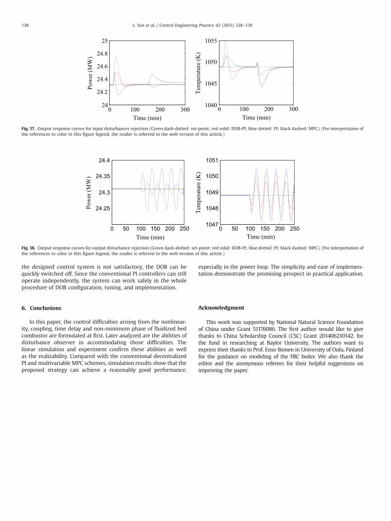
The frequent disturbances in FBC system, such as variations of heatvalue of feed coal, moisture content of primary air and erosion ofwater wall, may deteriorate the performance of feedback controlsystem significantly. In this part, the simulation is carried out byassuming the step disturbances imposed on the input port of feed coaland primary air at t¼20min and t¼150min, respectively. The closed-loop response curves of the output power and bed temperature areshown in Fig. 17.

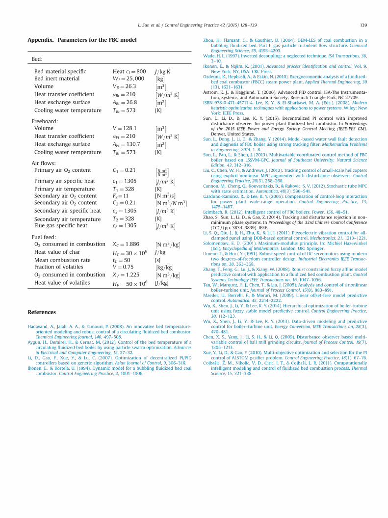
Another simulation is carried out by adding the sinusoidal externaldisturbances in the output ports. The corresponding response curvesare shown in Fig. 18. The dynamic behaviors of output power indicatethat DOB-based decentralized PI control achieved overwhelmingsuperiority over other methods in the power loop. Similar to theprevious phenomenon, DOB-based strategy did not perform as well asMPC in the temperature loop. The reason can be attributed to the NMPcharacteristic existing in the loop. Even with the suboptimal distur-bance estimation, the initial inverse estimation of disturbance is stillunavoidable, which will of course degrade the performance ofdisturbance rejection. However, as discussed in the previous section,it is not a wise decision to choose the MPC controller in this loop dueto the inconvenient configuration. If simplicity is of primary concern, it

is highly suggested to select the DOB-PI structure to achieve a balancebetween the performance and ease of use.

5.3. Discussion

The DOB-enhanced decentralized PI control can achieve super-ior performances to the conventional decentralized control inmost cases. Nonlinear plant can be compensated as linear nominalmodel, in particular in steady state and low-frequency region;coupling can be attenuated significantly; internal and externaldisturbances can be rejected in a timely manner.

Even though the control accuracy of the temperature loop is not asgood as MPC, it may be argued that the resulting temperature canalso be guaranteed within the safe region to avoid NOx formation. Interms of the practical implementation, only the lead–lag components,which can be easily found in the library of the current mainstreamDCS, is needed to configure the DOB module.

Another distinctive feature of the method that should beargued is the compatibility with the already running PI controllersand convenience for tuning. The tuning of DOB can be completedwithout incorporating the signal of disturbance estimation to thefeedback loop. Only after confirming the stability and reasonabilityof the estimation, the signal may be fed back to the closed-loop. If

Table 2Controller parametersa.

Controllers Tuning parameters

Decentralized PI Kp1¼0.04, Ti1¼200s, Kp2¼�0.01, Ti2¼909 sDOB enhanced Kp1¼0.04, Ti1¼200s, Kp2¼�0.01, Ti2¼909 sdecentralized PI T1¼100,Tf1 ¼15, λ1 ¼ 1:3, T2¼120State space Sampling time Ts¼10 s, prediction horizon (P)¼300, control horizon (M)¼20, weights on OV (Q)¼diag[1 0 1], Weights on MV (R)¼diag[1 0 1]).

Input saturation: [�2 2].MPC

a OV and MV are output variable and manipulated variable, respectively.

0 200 400 600 80024

25

26

27

28

29

Time (min)

Pow

er (M

W)

y 1:

0 200 400 600 8001000

1050

1100

1150

1200

Tem

pera

ture

(K)

Time (min)y 2

:

0 200 400 600 8002.8

3

3.2

3.4

3.6

3.8

Feed

Coa

l flo

w ra

te (k

g/s)

Time (min)

u 1:

0 200 400 600 8003

3.5

4

4.5

Time (min)

Prim

ary

air f

low

rate

(Nm

3 /s)

u 2:

Fig. 16. Control performance of continuous loading-up simulation (Green dash-dotted: set-point; red solid: DOB-PI; blue dotted: PI; black dashed: MPC). (For interpretationof the references to color in this figure legend, the reader is referred to the web version of this article.)

L. Sun et al. / Control Engineering Practice 42 (2015) 128–139 137

the designed control system is not satisfactory, the DOB can bequickly switched off. Since the conventional PI controllers can stilloperate independently, the system can work safely in the wholeprocedure of DOB configuration, tuning, and implementation.

6. Conclusions

In this paper, the control difficulties arising from the nonlinear-ity, coupling, time delay and non-minimum phase of fluidized bedcombustor are formulated at first. Later analyzed are the abilities ofdisturbance observer in accommodating those difficulties. Thelinear simulation and experiment confirm these abilities as wellas the realizability. Compared with the conventional decentralizedPI and multivariable MPC schemes, simulation results show that theproposed strategy can achieve a reasonably good performance,

especially in the power loop. The simplicity and ease of implemen-tation demonstrate the promising prospect in practical application.

Acknowledgment

This work was supported by National Natural Science Foundationof China under Grant 51176086. The first author would like to givethanks to China Scholarship Council (CSC) Grant 201406210142. forthe fund in researching at Baylor University. The authors want toexpress their thanks to Prof. Enso Ikonen in University of Oulu, Finlandfor the guidance on modeling of the FBC boiler. We also thank theeditor and the anonymous referees for their helpful suggestions onimproving the paper.

0 100 200 30024

24.2

24.4

24.6

24.8

25

Time (min)

Pow

er (M

W)

0 100 200 3001040

1045

1050

1055

Tem

pera

ture

(K)

Time (min)

Fig. 17. Output response curves for input disturbances rejection (Green dash-dotted: set-point; red solid: DOB-PI; blue dotted: PI; black dashed: MPC). (For interpretation ofthe references to color in this figure legend, the reader is referred to the web version of this article.)

0 50 100 150 200 250

24.25

24.3

24.35

24.4

Time (min)

Pow

er (M

W)

0 50 100 150 200 2501047

1048

1049

1050

1051

Tem

pera

ture

(K)

Time (min)

Fig. 18. Output response curves for output disturbance rejection (Green dash-dotted: set-point; red solid: DOB-PI; blue dotted: PI; black dashed: MPC). (For interpretation ofthe references to color in this figure legend, the reader is referred to the web version of this article.)

L. Sun et al. / Control Engineering Practice 42 (2015) 128–139138

Appendix. Parameters for the FBC model

Bed:

Bed material specific Heat cI ¼ 800 J=kg KBed inert material WI ¼ 25;000 kg

� �Volume VB ¼ 26:3 m3

� �Heat transfer coefficient αBt ¼ 210 W=m2 K

� �Heat exchange surface ABt ¼ 26:8 m2

� �Cooling water temperature TBt ¼ 573 K½ �

Freeboard:Volume V ¼ 128:1 m3

� �Heat transfer coefficient αFt ¼ 210 W=m2 K

� �Heat exchange surface AFt ¼ 130:7 m2

� �Cooling water temperature TBt ¼ 573 K½ �

Air flows:Primary air O2 content C1 ¼ 0:21 N m3

N m3

h iPrimary air specific heat c1 ¼ 1305 J=m3 K

� �Primary air temperature T1 ¼ 328 K½ �Secondary air O2 content F2¼11 [N m3/s]Secondary air O2 content C2 ¼ 0:21 N m3=N m3

� �Secondary air specific heat c2 ¼ 1305 J=m3 K

� �Secondary air temperature T2 ¼ 328 K½ �Flue gas specific heat cF ¼ 1305 J=m3 K

� �Fuel feed:O2 consumed in combustion XC ¼ 1:886 N m3=kg

� �Heat value of char HC ¼ 30� 106 J=kgMean combustion rate tC ¼ 50 s½ �Fraction of volatiles V ¼ 0:75 kg=kg

� �O2 consumed in combustion XV ¼ 1:225 N m3=kg

� �Heat value of volatiles HV ¼ 50� 106 ½J=kg�

References

Hadavand, A., Jalali, A. A., & Famouri, P. (2008). An innovative bed temperature-oriented modeling and robust control of a circulating fluidized bed combustor.Chemical Engineering Journal, 140, 497–508.

Aygun, H., Demirel, H., & Cernat, M. (2012). Control of the bed temperature of acirculating fluidized bed boiler by using particle swarm optimization. Advancesin Electrical and Computer Engineering, 12, 27–32.

Li, D., Gao, F., Xue, Y., & Lu, C. (2007). Optimization of decentralized PI/PIDcontrollers based on genetic algorithm. Asian Journal of Control, 9, 306–316.

Ikonen, E., & Kortela, U. (1994). Dynamic model for a bubbling fluidized bed coalcombustor. Control Engineering Practice, 2, 1001–1006.

Zhou, H., Flamant, G., & Gauthier, D. (2004). DEM-LES of coal combustion in abubbling fluidized bed. Part I: gas-particle turbulent flow structure. ChemicalEngineering Science, 59, 4193–4203.

Wade, H. L. (1997). Inverted decoupling: a neglected technique. ISA Transactions, 36,3–10.

Ikonen, E., & Najim, K. (2001). Advanced process identification and control. Vol. 9.New York, NY, USA: CRC Press.

Ozdemir, K., Hepbasli, A., & Eskin, N. (2010). Exergoeconomic analysis of a fluidized-bed coal combustor (FBCC) steam power plant. Applied Thermal Engineering, 30(13), 1621–1631.

Åström, K. J., & Hagglund, T. (2006). Advanced PID control. ISA-The Instrumenta-tion, Systems, and Automation Society; Research Triangle Park, NC 27709.

ISBN 978-0-471-45711-4. Lee, K. Y., & El-Sharkawi, M. A. (Eds.). (2008). Modernheuristic optimization techniques with applications to power systems. Wiley: NewYork: IEEE Press.

Sun, L., Li, D., & Lee, K. Y. (2015). Decentralized PI control with improveddisturbance observer for power plant fluidized bed combustor. In Proceedingsof the 2015 IEEE Power and Energy Society General Meeting (IEEE-PES GM).Denver, United States.

Sun, L., Dong, J., Li, D., & Zhang, Y. (2014). Model-based water wall fault detectionand diagnosis of FBC boiler using strong tracking filter. Mathematical Problemsin Engineering, 2014, 1–8.

Sun, L., Pan, L., & Shen, J. (2013). Multivariable coordinated control method of FBCboiler based on LSSVM-GPC. Journal of Southeast University: Natural ScienceEdition, 43, 312–316.

Liu, C., Chen, W. H., & Andrews, J. (2012). Tracking control of small-scale helicoptersusing explicit nonlinear MPC augmented with disturbance observers. ControlEngineering Practice, 20(3), 258–268.

Cannon, M., Cheng, Q., Kouvaritakis, B., & Raković, S. V. (2012). Stochastic tube MPCwith state estimation. Automatica, 48(3), 536–541.

Garduno-Ramirez, R., & Lee, K. Y. (2005). Compensation of control-loop interactionfor power plant wide-range operation. Control Engineering Practice, 13,1475–1487.

Leimbach, R. (2012). Intelligent control of FBC boilers. Power, 156, 48–51.Zhao, S., Sun, L., Li, D., & Gao, Z. (2014). Tracking and disturbance rejection in non-

minimum phase systems. In Proceedings of the 33rd Chinese Control Conference(CCC) (pp. 3834–3839). IEEE.

Li, S. Q., Qiu, J., Ji, H., Zhu, K., & Li, J. (2011). Piezoelectric vibration control for all-clamped panel using DOB-based optimal control. Mechatronics, 21, 1213–1221.

Solomentsev, E. D. (2001). Maximum-modulus principle. In: Michiel Hazewinkel(Ed.), Encyclopedia of Mathematics. London, UK: Springer.

Umeno, T., & Hori, Y. (1991). Robust speed control of DC servomotors using moderntwo degrees-of-freedom controller design. Industrial Electronics IEEE Transac-tions on, 38, 363–368.

Zhang, T., Feng, G., Lu, J., & Xiang, W. (2008). Robust constrained fuzzy affine modelpredictive control with application to a fluidized bed combustion plant. ControlSystems Technology IEEE Transactions on, 16, 1047–1056.

Tan, W., Marquez, H. J., Chen, T., & Liu, J. (2005). Analysis and control of a nonlinearboiler-turbine unit. Journal of Process Control, 15(8), 883–891.

Maeder, U., Borrelli, F., & Morari, M. (2009). Linear offset-free model predictivecontrol. Automatica, 45, 2214–2222.

Wu, X., Shen, J., Li, Y., & Lee, K. Y. (2014). Hierarchical optimization of boiler-turbineunit using fuzzy stable model predictive control. Control Engineering Practice,30, 112–123.

Wu, X., Shen, J., Li, Y., & Lee, K. Y. (2013). Data-driven modeling and predictivecontrol for boiler–turbine unit. Energy Conversion, IEEE Transactions on, 28(3),470–481.

Chen, X. S., Yang, J., Li, S. H., & Li, Q. (2009). Disturbance observer based multi-variable control of ball mill grinding circuits. Journal of Process Control, 19(7),1205–1213.

Xue, Y., Li, D., & Gao, F. (2010). Multi-objective optimization and selection for the PIcontrol of ALSTOM gasifier problem. Control Engineering Practice, 18(1), 67–76.

Ćojbašić, Ž. M., Nikolić, V. D., Ćirić, I. T., & Ćojbaši, L. R. (2011). Computationallyintelligent modeling and control of fluidized bed combustion process. ThermalScience, 15, 321–338.

L. Sun et al. / Control Engineering Practice 42 (2015) 128–139 139