Page 1
Control-Volume Based Navier,Stokes
Equation Solver Valid atAll Flow Velocities
lxl_ll_lt-S_IEI_ES _(,L_l_I_I£1i SCL_I_I_ _AI.IE AT ALt}LClm _ELECI_I_S (I_S_) LIE F CSC/_ _OO
_89-2C4(7
U_cla_
G3/3W 019_4_4
S.-W. Kim _ _ _
lr_titute for Computational Mechanics in Propulsion ......Lewis Research Center _ - ....
Cleveland, Ohio _
February 1989
https://ntrs.nasa.gov/search.jsp?R=19890011036 2020-04-13T22:30:24+00:00Z
Page 3
CONTROL-VOLUME BASED NAVIER-STOKES EQUATION SOLVER
VALID AT ALL FLOW VELOCITIES
S.-W. Kim*
Institute for Computational Mechanics in Propulsion
Lewis Research Center
Cleveland, Ohio 44135
SUMMARY
A control-volume based finite difference method to solve the Reynolds
averaged Navier-stokes equations is presented. A pressure correction
equation Valid at all flow velocities and a pressure staggered grid layout
are used in the method. Example problems presented herein include: a
developing laminar channel flow, a developing laminar pipe flow, a
lid-driven square cavity flow, a laminar flow through a 90-degree bent
channel, a laminar polar cavity flow, and a turbulent supersonic flow over
a compression ramp. A k-c turbulence model supplemented with a near-wall
turbulence model was used to solve the turbulent flow. It is shown that the
method yields accurate computational results even when highly skewed,
unequally spaced, curved grids are used. It is also shown that the method
is strongly convergent for high Reynolds number flows.
*Work funded under Space Act Agreement C99066G.
Page 4
A u
Av
A 1
A 2
A_
c2
c_f
dn
f_
fc
k
k e
km
k t
n
P
Pr
R
Re
R t
T
u T
V
x
y+
Nomenclature
coefficient for incremental u-velocity
coefficient for incremental v-velocity
constant coefficient for fp equation (-0.025)
constant coefficient for fp equation (-0.00001)
constant coefficient for f_ equation
turbulence model constants for _ equation, (2-1,2)
constant coefficient for eddy viscosity equation (-0.09)
normal distance from wall
wall damping function for eddy viscosity equation
wall damping function for _w equation
turbulent kinetic energy _!
effective thermal conductivity (-km_ t)
thermal conductivity
turbulent thermal conductivity (-CpPt/a T)
outward normal vector, (-{nx, ny})
pressure
production rate of turbulent kinetic energy
gas constant.
Reynolds number
turbulent Reynolds number (-k2/(VCl))
temperature
friction velocity (-J(_w/P))
velocity vector (=_u,v})
cartesian coordinates (-ix,y})
wall coordinate (-u_dn/w)
dissipation rate
Page 5
_W
#
_e
_t
V
vt
(_,_)
P
ak
oT
a_
fw
dissipation rate of turbulent kinetic energy
dissipation rate inside the near-wall layer
von Karman constant (-0.41)
molecular viscosity
effective viscosity (-_+_t)
turbulent viscosity
kinematic viscosity of fluid
turbulent eddy viscosity
curvilinear coordinates
density
turbulent Prandtl number for k-equation
turbulent Prandtl number for energy equation
turbulent Prandtl number for _-equation
wall shearing stress
dissipation function for energy equation
Superscripts
A
n
!
non-dimenslonal value normalized by the free stream value
iteration level
current value
incremental (or corrective) value
Subscripts
nb
P
neighboring grid points, (-{E, W, S, N})
grid point
Mathematical symbol
X summation
Page 6
INTRODUCTION
A control-volume based finite difference method to solve the Reynolds
averaged Navier-Stokes equations for all fl0w velocities is presented. The
method is an extension of the pressure correction method (SIMPLE) which is
used primarily to solve incompressible flows [1,2]. Numerical methods based
on the pressure correction method have been used extensively to solve
complex turbulent flows [3], including chemically reacting turbulent flows
[4], due to their strongly convergent nature. In the present study, a
pressure correction equation which is valid at all flow velocities is used
for numerical calculations of incompressible and compressible flows.
Many finite difference methods to solve the compressible flow
equations are based on the flux-splitting method. The Beam-Warming method
[5] and the McCormack method [6] are the representatives of the
flux-splitting methods. The flux-splitting methods were originally
developed to solve the Euler equations and then extended to include the
viscous term to solve the Navier-Stokes equations. The most distinguishing
practical difference between the pressure correction methods and the
flux-splitting methods lies in the way the diffusion term is treated. In
the former class of methods, the diffusion term has been incorporated into
the stiffness matrix while, in the latter class of methods, the diffusion
term has been incorporated into the system of equations as the load vector
term. For turbulent flows with extensive recirculation zones, the pressure
correction methods may be numerically more stable conceptually. However,
the pressure correction methods have mostly been used for incompressible
flows and the flux splitting methods have mostly been used for compressible
flows. Therefore, definitive advantages and disadvantages of these two
classes of methods can not be discussed with confidence as yet.
4
Page 7
The original numerical method based on the SIMPLE algorithm [2] is
used to solve the Navier-Stokes equations whose domain can be discretized
using orthogonal grids. A fully staggered grid layout [i] has been used in
the method. However, in many flow problems of practical importance, the
boundary geometries are complex and arbitrary shaped blockages may exist
inside the flow path. A number of papers to extend the pressure correction
methods for flows with arbitrary geometries and for compressible flows have
appeared in recent years [7-13].
A number of grid layouts have been proposed and tested to identify the
most suitable one to solve the Navier-Stokes equations defined on
arbitrary, complex geometries. In Reference 7, the standard fully staggered
grid layout, Figure l-(a), was used to solve the Navier-Stokes equations
defined on curved geometries. This grid layout can not be used to solve
flows inside 90-degree bent ducts (see Reference 8 for details). A
collocated grid layout, Figure l-(b), was used in References 9 and I0. In
Reference 9, the velocity - pressure decoupling was prevented by including
an artificial viscosity, while in Reference I0, the same purpose was
achieved by evaluating the incremental velocities at mld-sides of the
control volume. In Reference 8, the standard fully staggered grid was used
and the velocity vector was located at all grid points except at the
pressure grid point (see Figure l-(c)). In this case, the number of degrees
of freedom for velocity is doubled while that of pressure remains the same
as in the original case. Note that the accuracy of numerical solutions
depends not only on the number of velocity grid points but also on the
number of pressure grid points. Hence the accuracy can not be improved as
much as the doubled number of velocity grid points might suggest. In
References 12 and 13, the velocities were located at the same grid points
5
Page 8
and the pressure was located at the centroid of the cell formed by the four
adjacent velocity grid points (see Figure l-(d)). This grid layout has been
used successfully in penalty finite element methods for a long time [14].
It was first used in the control-volume based finite difference method in
Vanka et. al. [12]. They mentioned that it was not easy to obtain
convergent solutions due to the velocity-pressure decoupllng. The mechanism
that yields the velocity-pressure decoupled solution was heuristically
shown in Reference [8]. In Reference 13, the velocity-pressure decoupling
was eliminated by using a non-conforming domain for the mass imbalance
calculation. In the present study, the velocity-pressure decoupling was
eliminated by moving the off-diagonal terms to the load vector term. The
resulting system of equations was solved using the Tri-Diagonal Matrix
Algorithm (TDMA) [i]. Thus any uncertainty that may arise due to the use of
a non-conforming domain for the mass imbalance calculation does not exist
in the present method.
A few different numerical procedures have also been used to solve the
pressure correction equation for compressible flows. The SIMPLE-R [i] and
the SIMPLE-C [15] were used in References Ii and 13, respectively. The
pressure, velocity, and density were corrected based on the incremental
pressure (or pressure correction) in References ii and 13. In the present
study, only the pressure and velocity were corrected from the incremental
pressure as in the standard SIMPLE method [i]. Density was obtained from
the equation of state for perfect gas so that the same numerical procedure
could equally be applicable for numerical computations of chemically
reacting turbulent flows in the future. The numerical procedure to solve
the pressure correction equation for compressible flows may need to be
studied further in the future.
Page 9
A k-e turbulence model supplemented with a near-wall turbulence model
was used in the present study. Establishment of the near-wall turbulence
model and its application to fully developed turbulent channel and pipe
flows can be found in Reference 16. It has been shown in the reference that
the near-wall turbulence model can resolve the over-shoot phenomena of the
turbulent kinetic energy and the dissipation rate in the region very close
to the wall. Thus significantly improved computational results for the
near-wall turbulence structure were obtained. It is also shown in Reference
17 that the turbulence model yields correct location of the shock for a
transonic flow over an axisymmetric curved hill with shock wave - turbulent
boundary layer interaction [18].
A number of flow cases have been solved to test the accuracy and the
convergence nature of the present numerical method. The example flows
presented herein include: a developing laminar channel flow, a developing
laminar pipe flow, a lid-drlven square cavity flow [19-21], a
two-dimenslonal laminar flow in a 90-degree bent channel, a polar cavity
flow [22], and a turbulent supersonic flow over a compression ramp [23-24].
REYNOLDS AVERAGED NAVIER-STOKES EQUATIONS FOR COMPRESSIBLE FLOWS
The compressible turbulent flow equations are given as;
a a
--(pu) + --(pv) - O.ax ay
(1)
a a a a
--(puu) +--(p_) =_(rxx) +--(rxy)ax ay ax ay
ap
ax(2)
Page 10
a a a a ap
--(puv) +--(pvv) ---("yx) + --(ryy)ax ay ax ay ay
(3)
a a[keaTl [ko T1ax(pCpuT ) +--(pCpvT) ( axJ +ay ax ayL ayj
ap ap+u--+v--+_
ax ay
(4)
where
au 2#e
rxx - 2#eax 3
(v'V),
rxy - ryx - #e +I
av 2#e
ryy - 2# eay 3
(v'V),
@ - #e 21-- I + 2 -- + + --Layj axj
2#e
3---(v.v) 2,
au av
VoV -- __ + --,
ax ay
and the density is obtained from the perfect gas law given as p-pRT. The
turbulent Prandtl number (aT) of 0.75 was used for the energy equation in
the present calculations. The compressible turbulent flow equations for
axisymmetric case can be found in Reference 17.
The molecular viscosity and the thermal conductivity were obtained
Page 11
from the Sutherland's laws given as [25];
_o IT + S)
(5)
where #o - 1.716 x 10 .5 Kg/m-sec, To - 273.1 ° K, S - 110.6 ° K; and
k o IT + S)
<6)
where k o - 0.0264 Kg/m-K, To - 273.1 ° K, and S - 194.4 ° K.
TURBULENCE EQUATIONS
A k-¢ turbulence model supplemented with a near-wall turbulence model
is described below [16,17]. The turbulent kinetic energy equation for the
entire flow domain is given as;
_(puk) + i(pvk) - _ Pe + _ Pe-- + pPr -- pcax ay ax ay ay
(7)
where the production rate of turbulent kinetic energy (Pr) is the same as
the dissipation function for the energy equation (@).
The dissipation rate inside the near-wall layer is given as;
(W -- w
f_
(B)
where
9
Page 12
c_f3/4k3/2¢i
fe - i- exp(-AcRt)
k2Rt ---
c_f 3/2Ac
2_2
(9)
The dissipation rate given as eq. (8) is used for eq. (7) in the
near-wall region. The dissipation rate for the rest of the flow domain is
obtained by solving the convectlon-diffusion equation for the dissipation
rate equation given as;
--(pu_) +--(pvc) -- #e + e PCl PC2--
3x 3y 8x k k
(IO)
The turbulence model constants used are given as: ak-0.75 , a¢-i.15,
ci-1.39, and c2-1.88. These turbulence model constants approximately
satisfy the near-wall equilibrium turbulence condition and an
experimentally observed decay rate of the grid turbulence [26]. Further
discussion on the establishment of these constants can be found in
References 27-28.
The eddy viscosity inside the near-wall layer is given as;
i0
Page 13
k 2
u t - cpf fp- (ii)
where fp-l-exp(AiJR t + A2Rt 2) . The wall damping function fp is a linear
function of the distance from the wall in the viscous sublayer and becomes
unity in the fully turbulent region. The eddy viscosity, given as eq. (ii),
grows in proportion to the cubic power of the distance from the wall. The
eddy viscosity in the rest of the flow domain is given as;
k 2
v t = cpf- (12)
The partition between the near-wall region and the fully turbulent outer
region can be located between y+ greater than i00 and less than 300
approximately. Details on the k-_ turbulence model supplemented with the
near-wall turbulence model can be found in References 16 and 17.
NUMERICAL METHOD
In the present method, all flow variables, except pressure, have been
located at the same grid points and the pressure node has been located at
the ¢entroid of the cell formed by the four neighboring velocity grid
points. Note that in the control-volume methods based on pressure
correction methods, the discrete system of equations is derived by
integrating the governing differential equations over the control volume
[I]. For flows with arbitrary geometries, the number of interpolations to
obtain flow variables at the cell boundaries for the present grid layout is
as small as for any of the grid layouts discussed previously. Enhanced
convergence rate is partly attributed to the grid layout which requires
ll
Page 14
fewer interpolations.
The pressure correction equation for compressible flows is described
below. As in the standard pressure correction method [I], the dehsity, the
velocities, and the pressure are decomposedas;
* (13)p -- p + p'
* , (14)U--U +U,
* v' (15)V-- V + ,
* , (16)p-p +p
where the superscript * denotes the current values of the flow variables
which may not satisfy the conservation of mass equation yet. The discrete
momentum equation for u-veloclty can be written as;
ap
Apup - _ AnbUnb - -- + Sv uax
(17)
where Ap is the coefficient of the u-veloclty at the grid point P, Sv u is
the load vector originating from the curvillnear grid structure, and the
pressure gradient was left in continuous form deliberately. Substituting
eqs. (13-16) into eqs. (17) yields;
a(p*+p')
Ap(u*p+U'p) - X Anb(U*nb+U'nb) -- + Svu (18)ax
The discrete u-momentum equation based on the current flow variables which
may not satisfy the conservation of mass equation can be written as;
12
Page 15
ap*
ApU*p - _ AnbU*nb -- -- + Svu3x
(19)
Subtracting eq. (19) from eq. (18) yields;
3p'
U r m -- AH
3x
(20)
where Au-I/A p. In deriving eq. (20), the summation over the neighboring
grid points and the load vectors in eqs. (18) and (19) have been neglected.
The relationship between the incremental v-velocity and the pressure
gradient in the y-coordinate direction can be obtained by the same
procedure and is given as;
3p'
V e w -- Av --
3y
(21)
The incremental pressure is related to the incremental density as;
p' - p'RT (22)
where eq. (22) has been obtained from the equation of state. The
conservation of mass equation is given as;
v.(pv) - o
or,
v.(p'V*) + v-(p*v') + v.(p'v') - -v.(p*v*) (23)
13
Page 16
Substituting eqs. (20-22) into (23) yields, after some rearrangement;
(24)
where the higher order perturbation term v'(p'V') has been neglected in
deriving eq. (24). The last term in eq. (24) represents the mass imbalance.
Integrating eq. (24) over a pressure control volume yields;
f{ a,7 . a,7 ap'](25)
where the Green-Gauss theorem has been made use of to invert the volume
integration into a surface integration. The discrete control volume
equation for eq. (25) can be written as;
App'p - AEP' E + AWP' W + Asp' s + ANP' N +Scp, + Svp, (26)
where SCp, is a load vector of the mass imbalance and
SVp,-Afap'/a_+A_ap'/a_ contains all the contributions made by the
curvillnear grid. Note that the variable load vector Svp, is a null vector
in the first sweep. After the first sweep, the Svp, term was updated in
each sweep using the incremental pressure obtained in the previous sweep.
The other flow equations were solved by the same procedure as that of
Page 17
the pressure correction equation. However, the load vector Sv i
(i=u,v,t,k,_) is not a null vector and was evaluated only once in each
iteration. The upwind difference approximation [I] has been used to solve
the pressure correction equation; and the power law difference
approximation [I], for the other flow equations. The incremental pressure
is obtained by solving eq. (26), and the corresponding incremental
velocities are obtained from eqs. (20-21). The flow variables are updated
by using eqs. (14-16), and these updated flow variables are used in
computing the new current flow variables by solving eqs. (2-4) together
with the turbulence equations. The discrete finite difference system of
equations was solved iteratively using the TDMA until the residuals became
smaller than the prescribed convergence criteria. Each iteration consisted
of 7 sweeps of the pressure correction equation and 3 sweeps for the rest
of the flow equations in the flow direction and in the transverse
direction, respectively. The convergence criteria used are;
AA
C
R I - Iv'PVlc < e I (27)c-I
- (a n+l - a n ) An+lR2 I i,j i,j / i I < e2'
J-I,N, (28)
where N c is the number of control volumes for the pressure correction
equation; the subscript i-(u, v, p, T, k, _} denotes each flow variable;
the subscript j denotes each grid point; N denotes the number of degrees of
freedom for each flow variable; and A i denotes the maximum magnitude of the
i-th flow variable. The iteration was terminated when either eq. (27) or
eq. (28) was satisfied.
Each flow variable was updated using an under-relaxation factor [I].
15
Page 18
The under-relaxation procedure was incorporated into the systems of
equations for all flow equations except that of the pressure correction
equation. The pressure correction equation was solved without
under-relaxation; however, the pressure was obtained by adding the
incremental pressure multiplied by an under-relaxation factor. No symptom
that might lead to a velocity-pressure decoupled solution was observed in
the present method. For incompressible flows, R-l.0xlO 15 has been used in
eq. (24) or in eq. (25). Thus, elimination of the velocity pressure
decoupllng mechanism is achieved by the numerical method itself and has
nothing to do with the inclusion of the convection term into the pressure
correction equation.
COMPUTATIONAL RESULTS
The numerical method described in the previous sections was tested and
evaluated by solving a number of flow cases. Example flows presented herein
include: a developing laminar channel flow, a developing laminar pipe flow,
a lld-drlven square cavity flow [19-21], a two-dimenslonal laminar flow
through a 90-degree bent channel, a laminar polar cavity flow [22], and a
supersonic flow over a compression ramp with shock wave - turbulent
boundary layer interaction [23-24]. It is shown from the first three flow
cases that the present method does not yield any velocity-pressure
decoupled solution, and in fact, there was no symptom of the
veloclty-pressure decoupllng for any of the flow cases considered. The rest
of the flow cases were considered to test the accuracy, the convergence
nature, and the applicability of the present method to flow problems of
practical importance. Further application of the numerical method as well
as the turbulence model to a shock wave - turbulent boundary layer
16
Page 19
interaction in a transonic flow over an axisymmetric curved hill [18] can
be found in Reference 17.
Developing Laminar Channel Flow
A developing laminar channel flow at Re-25 is considered below. The
Reynolds number is based on the inlet velocity and the channel width. The
exit boundary was located at seven channel widths downstream of the inlet.
Uniform velocity was prescribed at the inlet boundary; and vanishing
gradient boundary condition for velocities, at the exit boundary. The flow
domain was discretized by an equally spaced mesh as well as by an unequally
spaced mesh with 41 grid points in the flow direction and 26 in the
transverse direction in each case. The unequally spaced mesh is shown in
Figure 2-(a). The convergence criteria used were el-e2-1.0xl0 "4 and the
converged solution was obtained after approximately 410 iterations. The
residuals at the time of convergence were Ri-9.4x10 "5 and R2-1.1xl0 "4 The
calculated velocity profile at the exit boundary is compared with the exact
solution in Figure 2-(b). It can be seen in the figure that the present
method almost yields the exact solution.
Developing Laminar Pipe Flow
A developing laminar pipe flow at Rem25 was solved to test the
possible existence of the velocity-pressure decoupling for the axisymmetric
flow case. The Reynolds number is based on the inlet velocity and the
radius of the pipe. The exit boundary was located at seven radii downstream
of the inlet. An equally spaced mesh and an unequally spaced mesh with
41x26 grid points were used as in the previous case. The unequally spaced
mesh is shown in Figure 3-(a). The boundary conditions, the initial guess,
17
Page 20
and the convergence criteria used are the same as in the previous channel
flow case. The converged solution was obtained after approximately 170
iterations and the residuals at the time of convergence were Ri-4.2xlO'4
and R2-9.1x10 "5. Again, it can be seen in Figure 3-(b) that the present
method almost yields the exact solution.
Lid-Dr%yen Scuare Cavity Flow
A lid-driven cavity flow at Re-1000 is considered below to further
confirm that the present numerical method is free of the velocity -pressure
decoupllng mechanism. As a remark, the computational results obtained by
the finite difference methods using fine grids can be found in References
19 and 20 and those obtained by a finite element method can be found in
Reference 21. The computational domain was discretlzed by an unequally
spaced 81 X 81 mesh with concentration of the grid points in the near wall
region. The boundary conditions and the initial guess used are the same as
in Reference 21. The converged solution was obtained after approximately
590 iterations for el-e2-1.OxlO -4. The residuals at the time of convergence
were Ri-2.0xl0 "4 and R2-1.0xl0 "4. The calculated streamline contour is
shown in Figure 4. It can be seen in the figure that the secondary vortices
in the bottom corners were accurately resolved by the present method.
Two-Dimenslonal Laminar Flow Th[Qugh a 90-Degree Bent Channel
A two-dlmenslonal laminar flow through a 90-degree bent channel for
Re-1000 is considered below. The Reynolds number is based on the channel
width and the bulk velocity. It is shown from this flow case that the
present numerical method can solve flows with arbitrary geometries as
easily as flows with rectangular geometries. Note that the numerical
18
Page 21
methods adopting the fully staggered grid layout and solving for the
cartesian velocities can not be used to solve this flow case. The inlet
boundary was located at 5 channel widths upstream of the curved section;
and the exit boundary, at 15 channel widths downstreamof the curved
section. The flow domainwas discretized by 71 grid points in the flow
direction and 25 in the transverse direction. The velocity profile of a
fully developed channel flow was prescribed at the inlet boundary. The
vanishing gradient boundary condition was used for velocities at the exit
boundary. The convergence criteria used were el-e2-1.0xlO'4. The converged
solution was obtained after approximately 500 iterations. The residuals at
the time of convergence were Ri-8.3x10 "2 and R2-1.0xl0 -4. The mass flow
rate, obtained from the prescribed inlet velocity profile, through the
inlet boundary was 0.814419 Kg/m-sec and the calculated mass flow rate
leaving the exit boundary was 0.814401 Kg/m-sec. Hence the relative mass
imbalance was 2.2xi0 -5. The grids, the calculated streamline contour, and
the pressure contour in the vicinity of the curved section for Re-1000 is
shown in Figure 5.
Lamina_ Pol_r Cavity Flow
A laminar polar cavity flow at Re-60 and 350 is considered below to
test the accuracy of the present numerical method. The Reynolds number is
based on the azimuthal velocity and the radius of curvature of the lid. The
polar cavity is schematically shown in Figure 6. The experimental data can
be found in Reference 22. The flow domain was discretized by 81x81 grid
points, as in the Reference 22, with concentration of grid points in the
corner regions. The Dirichlet boundary condition for velocities was
prescribed at all boundaries. The convergence criteria used were
19
Page 22
el-e2-4.0xl0"5 For Re-60, the =onverged solution was obtained after
approximately 810 iterations and the residuals were Rl-l.5xlO-3 and
R2-3.9xlO'5. For Re-350, the converged solution was obtained after
approximately 820 iterations and the residuals at the time of convergence
were Ri-7.1xlO'3 and R2-3.7xlO-5. In each case, the required computational
time was approximately 8 minutes for the CRAY/XMP at the NASA/LeRC.
The calculated azimuthal and radial velocity profiles at three
azimuthal locations for Re-60 are compared with experimental data as well
as the computational results of Reference 22 in Figures 7-(a) and 7-(b),
respectively. It can be seen that the present computational results and
those obtained using the standard SIMPLE method [22] compare favorably with
experimental data. The present method yielded a slightly better radial
velocity profile at 8-20 degrees as shown in Figure 7-(b). The calculated
streamline, pressure, and the vorticity contours are shown in Figure 8. It
can be seen from the pressure contour and the vorticlty contour that the
potential core has not been well established at Re-60.
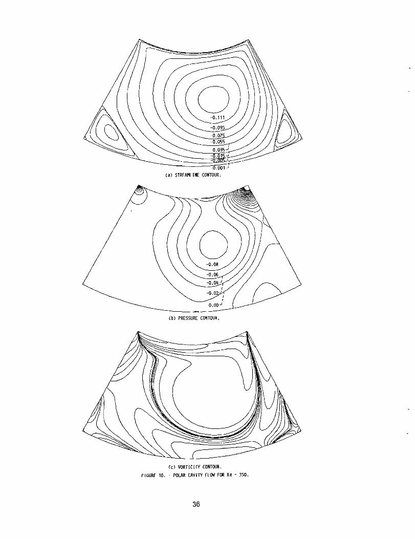
The calculated azimuthal and radial velocity profiles at the same
three azimuthal locations for Re-350 are compared with experimental data as
well as those of Reference 22 in Figure 9. It can be seen in the figure
that both computational results are in good agreement with the experimental
data. It is mentioned in Reference 22 that the first order differencing
method yielded inaccurate computational results for the polar cavity flow
at Re-350. However, it can be seen in the figure that the present method
yielded a_ accurate computational results as those obtained using the
second order differencing method of Reference 22. It can be seen from the
pressure and the vortlcity contours that the potential core has been well
established at Re-350.
20
Page 23
Turbulent Supersonic Flow over a Compression Ramp
A turbulent supersonic flow over a 24-degree compression ramp is
considered below. The experimental data can be found in References [23-24].
The free stream Mach number was 2.85, the boundary layer thickness of the
approaching supersonic flow was 0.0211 meters, and the Reynolds number
based on the free stream condition and the boundary layer thickness was
1.13xlO 6 .
In the numerical calculation, the inlet boundary was located at 2.17
boundary layer thicknesses upstream of the corner; and the exit boundary,
at five boundary layer thicknesses downstream of the corner. The top
boundary was located at seven boundary layer thicknesses away from the
wall. The flow domain was discretized by 97 grid points in the flow
direction and 56 in the transverse direction. The partition between the
near-wall layer and the external region was located at approximately 4.5
per cent of the boundary layer thickness away from the wall and 14 grid
points were allocated inside the near-wall layer. The grid size in the
normal direction was increased by a factor of approximately 1.2. The inlet
boundary condition for the tangential velocity and the turbulent kinetic
energy were obtained from experimental data for a fully developed flat
plate flow [29]. The non-dimensional velocity and the turbulent kinetic
energy profiles were scaled to yield a boundary layer thickness of 0.0211
meters at the inlet boundary. Uniform static pressure and uniform enthalpy
were also prescribed at the inlet boundary. The no-slip boundary condition
for velocities, vanishing turbulent kinetic energy, and a constant
temperature which corresponds to the free stream stagnation temperature
were prescribed at the solid wall boundary. The free stream flow condition
21
Page 24
was prescribed at the top boundary, and the vanishing gradient boundary
condition was used for all flow variables at the exit boundary. The initial
guess was obtained by extending the inlet boundary condition in the flow
direction. The converged solution was obtained after approximately 1400
iterations for el-e2-4.0x10"4. At the time of convergence RI and R2 were
3.5xi0 -4 and 4.0x10 "4, respectively. The mass flow rate through the inlet
boundary, obtained from the prescribed inlet boundary conditions, was
68.434 Kg/m-sec and the calculated mass flow rate leaving the exit boundary
was 68.411 Kg/m-sec. Hence the relative mass imbalance was 3.4xi0 "4. The
required computational time was approximately 18 minutes for the CRAY/XMP
at the NASA/LeRC.
The calculated static pressure on the wall is comparedwith
experimental data as well as the computational result obtained using a
relaxation turbulence model [24] in Figure ii. In Reference 24, several
sets of computational results obtained using various turbulence models were
presented. The wall pressure obtained using a relaxation turbulence model
[24] comparedmost favorably with the experimental data. It can be seen in
the figure that the present turbulence model yielded slightly compressed
pressure distribution. The level of agreementbetween the experimental data
and all the other computational results of Reference 24 was almost the same
as that of the present computational result.
The meanvelocity profiles at s/6--2.17, 0.0, and 2.89 are compared
with experimental data as well as with those obtained using the relaxation
turbulence model [24] in Figure 12, where the distance (s) has been
measured from the corner along the surface and 6 is the boundary layer
thickness. It can be seen that the present computational results compare
more favorably with the experimental data than does the other computational
22
Page 25
result [24]. The level of agreement between the best computational result
in Reference 24 and the experimental data was almost the same as that of
the present case. Note that the velocity profiles obtained using the
relaxation model compared less favorably with the experimental data than
those obtained using the other turbulence models [24].
The calculated streamline contour is shown in Figure 13-(a). The
measured flow separation zone extended from s/6=-1.44 to s/6=0.5. The
present method yielded the flow reclrculation zone extending from s/6--0.72
to s/6-0.68. The levels of agreement between the measured flow
reclrculatlon zone and all the computational results, including the present
result, were almost the same. However, the relaxation model which yielded
the best wall pressure yielded the worst flow reclrculatlon zone. The
calculated static pressure contour lines are shown in Figure 13-(b), where
the pressure has been normalized by the inlet total pressure and the
incremental pressure betweenthe contour lines is 0.2. The calculated
iso-Mach lines and the turbulent kinetic energy contours are shown in
Figures 13-(c) and 13-(d), respectively. The incremental Mach number
between the iso-Mach lines is 0.2 in Figure 13-(c). It has been shown in
this example that the present computational result compared as favorably
with the experimental data as any other computational results [24].
CONCLUSIONS
A control-volume based finite difference method to solve the Reynolds
averaged Navler-Stokes equations for all flow velocities has been
presented.
It has been shown from the developing channel flow, the developing
pipe flow, and the lid-driven square cavity flow that the present numerical
23
Page 26
method is free of the velocity-pressure decoupllng. For the channel and the
pipe flows, the method almost yields the exact solutions. For the polar
cavity flow, the present method yielded as accurate computational results
as the second order differencing method [22]. The turbulent supersonic flow
over the 24-degree compression ramp [23-24] was solved using a k-_
turbulence model supplemented with a near-wall turbulence model, In the
method, the dissipation rate inside the near-wall region was obtained from
an algebraic equation and that for the rest of the flow domain was obtained
by solving the differential equation for the dissipation rate. This
approach was found to be more advantageous than the low Reynolds number
turbulence models since the stiff dissipation rate equation in the
near-wall region need not be solved numerically. The computational results
for the supersonic compression corner flow compared as favorably with the
experimental data as any other computational results [24].
It has also been shown that the present numerical method yields
accurate computational results even when highly skewed, unequally spaced,
curved grids were used. Equally importantly, the present method was found
to be strongly convergent for high Reynolds number flows as well as for
flows with complex geometries. This strongly convergent nature is
attributed, in part, to the use of the pressure staggered grid layout.
24
Page 27
1. Patankar, S.V.:
York, 1980.
REFERENCES
Numerical Heat Transfer and Fluid Flow. McGraw-Hill, New
2. Gosman, A.D.; and Ideriah, F.J.K.: TEACH-T, Department of Mechanical
Engineering, Imperial College, London, 1982.
3. Kline, S.J.; Cantwell, B.J.; and Lilley, G.M. eds.: Complex Turbulent
Flows, Vols. 1-3, Mechanical Engineering Dept., Stanford University, 1981.
4. Jones, W.P.; and Whitelaw, J.H.: Calculation Methods for Reacting
Turbulent Flows: A Review." Combust. Flame, vol. 48, no. i, Oct. 1982,
pp. 1-26.
5. Beam, R.M.; and Warming, R.F.: An Implicit Factored Scheme for the
Compressible Navier-Stokes Equations. AIAA J., vol. 16, no. 4, Apr. 1978,
pp. 393-402,
6. MacCormack, R.W.: A Numerical Method for Solving the Equations of
Compressible Viscous Flow. AIAA J., vol. 20, no. 9, Apr. 1982,
pp. 1275-1281.
7. Shyy, W.; Tong, S.S.; and Correa, S.M.: Numerical Recirculating Flow
Calculation Using a Body-Fitted Coordinate System. Numerical Heat
Transfer, vol. 8, no. I, 1985, pp. 99-113.
8. Maliska, C.R.; and Raithby, G.D.: A Method for Computing Three
Dimensional Flows Using Non-Orthogonal Boundary-Fitted Coordinates. Int.
J. Numer. Methods Fluids, vol. 4, no. 6, June 198_, pp. 519-537.
9. Rhie, C.M.: A Pressure Based Navier-Stokes Solver Using the Multlgrid
Method. AIAA Paper 86-0207, Jan. 1986.
I0 Dwyer; H.A.; and Ibrani, S.: Time Accurate Solutions of the Incompressible
and Three-Dimensional Navier-Stokes Equations. AIAA Paper 88-0418, Jan.
1988.
25
Page 28
Ii. Karkl, K.C.; and Patankar, S.V.: A Pressure Based Calculation Procedure
for Viscous Flows at All Speeds in Arbitrary Configurations. AIAA
Paper 88-0058, Jan. 1988.
12. Vanka; S.P.; Chen, B.C.J.; and Sha, W.T.: A Semi-Implicit Calculation
Procedure for Flows Described in Boundary-Fitted Coordinate Systems.
Numerical Heat Transfer, vol. 3, no. i, 1980, pp. 1-19.
13. Chen, Y.S.: Viscous Flow Computations Using a Second-Order Upwind
Differencing Scheme. AIAA Paper 88-0417, Jan. 1988.
14. Fortin, M.; and Fortin, A.: Newer and Newer Elements for Incompressible
Flow. Finite Elements in Fluids, vol. 6, R.H. Gallagher, et al., eds.,
J. Wiley and Sons, New York, 1985, pp. 171-187.
15. Raithby, G.D.; and Schneider, G.E.: Numerical Solution of Problems in
Incompressible Fluid Flow: Treatment of the Velocity-Pressure Coupling.
Numerical Heat Transfer, vol. 2, no. 4, 1979, pp. 417-440.
16. Kim, S.W.: A Near-Wall Turbulence Model and Its Application to Fully
Developed Turbulent Channel and Pipe Flows. NASA TM-I01399, 1988.
17. Kim, S.W.: Numerical Computation of Shock Wave - Turbulent Boundary Layer
Interaction in Transonic Flow Over an Axisymmetric Curved Hill. NASA
TM-I01473, 1989.
18. Johnson, D.A.; Horstman, C.C.; and Bachalo, W.D.: Comparison Between
Experiment and Prediction for a Transonic Turbulent Separated Flow. AIAA
J., vol. 20, no. 6, June 1982, pp. 737-744.
19. Ghia, U.; Ghia, K.N.; and Shin, C.T.: High-Re Solutions for Incompressible
Flow Using the Navier-Stokes Equations and a Multigrid Method. J. Comput.
Phys., vol. 48, no. 3, Dec. 1982, pp. 387-411.
20. Schreiber, R.; and Keller, H.B.:
Numerical Techniques. J. Comput
pp. 310-333.
Driven Cavity Flows by Efficient
Phys., vol. 49, no. 2, Feb. 1983,
26
Page 29
21. Kim, S.W.: A Fine Grid Finite Element Computation of Two-Dimensional High
Reynolds NumberFlows. Computers Fluids, vol. 16, no. 4, 1988,
pp. 429-444.
22. Fuchs, L.; and Tillmark, N.: Numerical and Experimental Study of Driven
Flow in a Polar Cavity. Int. J. Numer. Methods Fluids, vol. 5, no. 4,
Apr. 1985, pp. 311-329.
23. Settles, G.S.; Vas, I.E.; and Bogdonoff, S.M.: Details of a Shock-
Separated Turbulent Boundary Layer at a CompressionCorner. AIAA J.,
vol. 14, no. 12, Dec. 1976, pp. 1709-1715.
24. Horstman, C.C., et al.: Reynolds NumberEffects on Shock-Wave
Turbulent-Boundary Layer Interactions. AIAA J., vol. 15, no. 8, Aug.
1977, pp. 1152-1158.
25. White, F.M.: Viscous Fluid Flow.
26. Harlow, F.H.; and Nakayama,P.I.:
McGraw-Hill, NewYork, 1974.
Transport of Turbulence Energy Decay
Rate. LA-3854, Los Alamos Scientific Lab, 1968.
27 Kim, S.W.; and Chen, Y.S.: A Finite Element Computation of Turbulent
Boundary Layer Flows with an Algebraic Stress Turbulence Model. Comput.
Methods Appl. Mech. Eng., vol. 66, no. i, 1988, pp. 45-63.
28 Kim, S.W.; and Chert, C.P.: A Multiple-Time-Scale Turbulence Model Based
on Variable Partitioning of the Turbulent Kinetic Energy Spectrum. To
appear in Numerical Heat Transfer, 1989. (Also available as NASA
CR-179222, 1987; and AIAA Paper 88-0221, 1988).
29. Klebanoff, P.S.: Characteristics of Turbulence in a Boundary Layer with
Zero Pressure Gradient. NACAReport 1247, 1955.
27
Page 30
V
TU
0
I
(a)FULLYSTAGGEREDGRID.
(b) COLLOCATEDGRID.
• )
(c) EXTENDEDFULLYSTAGGEREDGRID.
0
J_/ (U,V)
J
(d) PRESSURESTAGGEREDGRID.
FIGUREI. - GRIDLAYOUTS,
28
Page 31
1.0
>, .5
(a) LI1 x 26 GRID.
COMPO'ATI ";LoL;E/OoLNT
1
U
(b) VELOCITY PROFILE.
FIGURE 2, - DEVELOPING LAMINAR CHANNEL FLOW.
(a) 41 x 2(; GRID.
1.0
.5
COMPUTATIONAL RESULT
1 2
u
(b) VELOCITY PROFILE.
FIGURE 3, - DEVELOPING LAMINAR PIPE FLOW.
29
Page 32
\
FIGURE 4. - STREAMLINE CONTOUR FOR LID-ORIVEN CAVITY FLOW AT Re = 1000.
3O
Page 33
(a) GRID.
(b) STREAMLINE CONTOUR.
(C) PRESSURE CONTOUR.
FIGURE 5. - LAMINAR FLOW THROUGH A 90-DEGREE BENT CHANNEL.
31
Page 34
U8 = 1,0
ry
8
0=
FIGURE 6, - POLAR CAVITY FLOW.
32
Page 35
1. O0
.75
.50 --
.25 --
0-0.5
1.00 --
.75 --
.50 --
.25 --
0
-0.50
PRESENT COMPUTATIONAL RESULT
COMPUTATIONAL RESULT [22I
0 EXPERIMENTAL DATA [22]
0 = 20 0 -20
o o
I0 .5
u e
(a) AZIMUTHAL VELOCITY.
O = 20
f
I .__I-0.25 0
0 -20
0 0 .25
Ur
(b) RADIAL VELOCITY PROFILE.
FIGURE 7. - POLAR CAVITY FLOW FOR Re : 60.
I1.0
J,50
33
Page 36
(a) STREAMLINE CONTOUR.
(b) PRESSURECONTOUR.
(c) VORTICITY CONTOUR,
FIGURE 8. - POLARCAVITY FLOWFOR Re = GO.
34
Page 37
1.00
,75
_" ,50
.25
0-o.5
PRESENT COMPUTATIONAL RESULT
..... COMPUTATIONAL RESULT [22I
0 EXPERIAMENTAL DATA [22]
0 - 20 0 -20
I0 O 0 .5 1.0
u0
(a) AZIMUTHAL VELOCITY.
1,00
.75
.50 --
,25 --
0-0.50
8 = 20 0
0
0
©
0
/-0.25 0 0
uf
-20
I0 ,25
(b) RADIAL VELOCITY PROFILE,
FIGURE 9. - POLAR CAVITY FLOW FOR Re = 350,
I•50
35
Page 38
-0.001-_
(a) STREAMLINE CONTOUR.
(b) PRESSURE CONTOUR.
(c) VORTICITY CONTOUR.
FIGURE 10. - POLAR CAVITY FLOW FOR Re = 350.
36
Page 39
5,0 --
82.5
f _y,,O
,/,,sO
#'#@
s"'''-'C_Y _ PRESENT COMPUTATIONAL RESULT
Is 0 _ ----- COMPUTATIONAL RESULT [24]
fO 'f 0 EXPERIMENTAL DATA [23-24]
I I I-2.5 0 2.5 5.0
X/5
F]GURE 11. - STATIC _LL PRESSURE F_ COMPRESSIOM CORNER FLOW.
•05o
.025
0
PRESENT COMPUTATIONAL RESULT
COMPUTATIONAL RESULT [241
EXPERIMENTAL DATA [23-2q]
S/6 -2.17 S/_ 0 S/6 : 2,89
,6_ I I.o-0 ,7 0 .7
U/Uoo
FIGURE 12. - VELOCITY PROFILES FOR COMPRESSION CORNER FLOW.
37
Page 40
(a) STREABL[NE CONTOUR.
(b) PRESSURE CONTOUR.
(c) ISO-MACH LINES.
(d) TURBULENT KINETIC ENERGY CONTOUR.
FIGURE 13, - COMPRESSION CORNER FLOW.
38
Page 41
Report Documentation PageNationalAeronauticsandSpace Administration
1. Report No. NASA TM-101488 2. Government Accession No, 3. Recipient's Catalog No.
ICOMP-89-5
5. Report Date4. Title and Subtitle
Control-Volume Based Navier-Stokes Equation SolverValid at All Flow Velocities
7. Author(s)
S.-W. Kim
9, Performing Organization Name and Address
National Aeronautics and Space AdministrationLewis Research Center
Cleveland, Ohio 44135-3191
12. Sponsoring Agency Name and Address
National Aeronautics and Space Administration
Washington, D.C. 20546-0001
February 1989
6. Performing Organization Code
8. Performing Organization Report No.
E-4629
10. Work Unit No.
505-62-21
11. Contract or Grant No.
13. Type of Report and Period Covered
Technical Memorandum
14. Sponsoring Agency Code
i15. Supplementary Notes
S.-W. Kim, Institute for Computational Mechanics in Propulsion, NASA Lewis Research Center (work funded
under Space Act Agreement C99066G).
16. Abstract
A control-volume based finite difference method to solve the Reynolds averaged Navier-Stokes equations is
presented. A pressure correction equation valid at all flow velocities and a pressure staggered grid layout areused in the method. Example problems presented herein include: a developing laminar channel flow, developing
laminar pipe flow, a lid-driven square cavity flow, a laminar flow through a 90-degree bent channel, a laminar
polar cavity flow, and a turbulent supersonic flow over a compression ramp. A k-e turbulence model supplementedwith a near-wall turbulence model was used to solve the turbulent flow. It is shown that the method yields
accurate computational results even when highly skewed, unequally spaced, curved grids are used. It is also
shown that the method is strongly convergent for high Reynolds number flows.
17. Key Words (Suggested by Author(s))
Control volume method
Near wall turbulence model polar cavity flow
Turbulent flow over compression range
18. Distribution Statement
Unclassified- Unlimited
Subject Category 34
19. Security Classif. (of this report) 20. Security Classif. (of this page) 21. No of pages
Unclassified Unclassified 40
NASA FORM 1626 OCT 86*For sale by the National Technical Information Service, Springfield, Virginia 22161
22. Price"
A03