MCAT Institute Final Report 94-004 NASA-CR-195094 / J, / DEVELOPMENT OF ADVANCED NAVIER-STOKES SOLVER Seokkwan Yoon (NASA-CR-195094) DEVELOPMENT ADVANCED NAVIeR-STOKES SOLVER (MCAT Inst.) 20 p OF N94-37449 unclas G3/64 0016036 June 1994 NCC2-505 MCAT Institute 3933 Blue Gum Drive San Jose, CA 95127 https://ntrs.nasa.gov/search.jsp?R=19940032941 2019-02-21T20:30:17+00:00Z
Multigrid Convergence of an Implicit SymmetricRelaxation Scheme
Seokkwan Yoon* and Dochan Kwak?
NASA Ames Research Center, Moffett Field, California 94035
The multigrid method has been applied to an existing three-dimensional compressible Euler solver toaccelerate the convergence of the implicit symmetric relaxation scheme. This lower-upper symmetric Gauss-Seidel implicit scheme is shown to be an effective multigrid driver in three dimensions. A grid refinement studyis performed including the effects of large cell aspect ratio meshes. Performance figures of the present multigrid
code on Cray computers including the new C90 are presented. A reduction of three orders of magnitude in theresidual for a three-dimensional transonic inviscid flow using 920 k grid points is obtained in less than 4 min ona Cray C90.
I. Introduction
LTHOUGH unstructured grid methods have been usedsuccessfully in solving the Euler equations for complex
geometries, structured grid solvers still remain useful for the
Navier-Stokes equations because of their natural advantages
in dealing with the highly clustered meshes in the viscous
boundary layers. Structured grid methods not only handle
reasonably complex geometries using multiple blocks but also
offer a hybrid grid scheme to alleviate difficulties which un-structured grid methods have often encountered. Recent de-
velopments in structured grid solvers have been focused on
efficiency, as well as accuracy, since most existing three-di-
mensional Navier-Stokes codes are still not efficient enough to
be used routinely for aerodynamic design.
Multigrid methods have been useful for accelerating the
convergence of iterative schemes. Efficient Euler codes havebeen developed by Jameson t using a full approximation stor-
age method of Brandt z in conjunction with the explicit Runge-
Kutta scheme. The explicit multigrid method has demon-
strated impressive convergence rates by taking large time steps
and propagating waves fast on coarse meshes. The explicitmultigrid method has been extended to the Navier-Stokes
equations by Martinelli. 3 Several explicit multigrid codes for
the three-dimensional Navier-Stokes equations have been de-
veloped successfully by Vatsa and Wedan, 4 Radespiel et al., 5and Turkel et al.6
It does not seem to be pr(afit-able to consider an unfactored
implicit scheme for a multigrid driver since the implicit scheme
can take large time steps which are limited by the physics rather
than the grid. However, the multigrid method can improve the
convergence rates of factored implicit schemes in two dimen-sions as demonstrated by Yoon 7 and in Refs. 8-10. The im-
plicit multigrid method has been implemented by Caughey ]2 to
the diagonalized alternating direction scheme, i t and by Ander-son et alY to the three-dimensional alternating direction
scheme. Yoon 7 has introduced an implicit algorithm based on
a lower-upper (LU) factorization and symmetric Gauss-Seidel
(SGS) relaxation. The scheme has been used successfully in
*Research Scientist, Computational Algorithms and ApplicationsBranch.
t-Chief, Computational Algorithms and Applications Branch.
computing chemically reacting flows due in part to the al-
gorithm's property which reduces the size of the left-hand sidematrix for nonequilibrium flows with finite rate chemis-
try. t4-t6 A recent study t7 shows that the three-dimensional
extension of the method using a single grid requires less com-
putational time than most existing codes on a Cray YMP
computer. One of the objectives of the present work is to
accelerate the convergence of the lower-upper symmetricGauss-Seidel relaxation scheme in three dimensions by intro-
ducing a multigrid technique. The performance of the code is
demonstrated for an inviscid transonic flow past an ONERA
M6 wing on highly clustered grids.
II. Governing Equations
Let t be time; _ the vector of conserved variables;/_, P', and(_ the convective flux vectors; and -_, Pv, and (_, the flux
vectors for the viscous terms. Then the three-dimensional
Navier-Stokes equations in generalized curvilinear coordinates
(/_, 71, _') can be written as
atL)+ a_(_"- $.)+ o.(P-t'.)+ ago - 0,) = o (1)
where the flux vectors are defined in Ref. 17. The Euler
equations are obtained by neglecting the viscous terms.
950
III. Lower-Upper Symmetric Gauss-SeidelImplicit Scheme
An unfactored implicit scheme can be obtained from a
nonlinear implicit scheme by linearizing the flux vectors about
the previous time step and dropping terms of the second and
higher order.
[I + ez%t(Di_t + D_]3 + D_')I6Q = -_t_ (2)
where the residual/_ is
(3)
and I is the identity matrix. The correction _Y' + 1 _ _, is _.,
where n denotes the time level. DI, D r, and D r are differenceoperators that approximate a t, a_, and a¢, respectively. ,,_,/),and _7 are the Jacobian matrices of the convective flux vectors.
For a = IA, the scheme is second-order accurate in time. For
other values of _, the time accuracy drops to first order.
An efficient implicit scheme can be derived by combining
the advantages of LU factorization and Gauss-Seidel relaxation.
LD - ' U6_ = - At2_ (4)
HMliK;IU, Ww4i PAGE BLANK NOT FILMED
Here,
L = I + c_At(D_-_* +D_-B ÷ +DF_ + -.?4- -B--O-)
D= l + ou_t(_l ÷ - 21- + [3* -[3- + _* -dr-) (5)
U = I +_z_t(D_+71- + D;[3- +D(O- +A * +[3+ + _*)
where D(, D,-, and D:- are backward difference operators,
while D(, D_+, and D_+ are forward difference operators.
In the framework of the LU-SGS algorithm, a variety ofschemes can be developed by different choices of numerical
dissipation models and Jacobian matrices of the flux vectors.
Jacobian matrices leading to diagonal dominance are con-
structed so that + matrices have non-negative eigenvalues
whereas - matrices have nonpositive eigenvalues. For example,
(6)
where typically T_ and 7"_- 1 are similarity transformation ma-
trices of the eigenvectors of ,4. Another possibility is to con-
struct the Jacobian matrices of the flux vectors approximatelywhich yield diagonal dominance.
,21* = ½[.21 + k(_l)ll
[3- = ,/2[[3+ k([3)II (7)
dr* = ½ [dr + _(d3II
Here, the conserved variables are averaged at the cell faces to
evaluate the fluxes. The dissipative flux d is added to theconvective flux in a conservative manner.
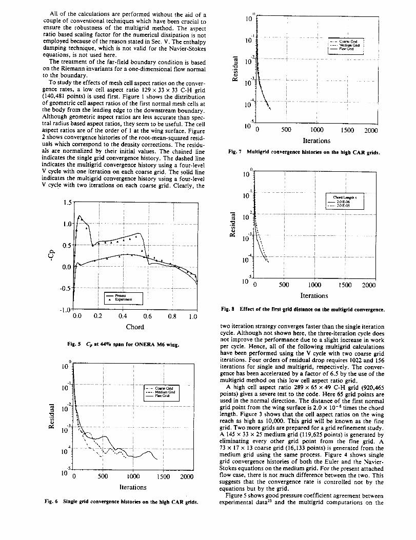
Fig. 4 Convergence histories for the Euler and Navier-Stokes equa-tions.
The process is repeated on successively coarser grids. Multiple
iterations can be done on each coarse grid. Finally, the correc-
tion calculated on each grid is interpolated back to the next
finer grid. Let _.2, be the final value of Q_ resulting from both
the correction calculated on grid 2h and the correction trans-
ferred from the grid 4h. Then
_ = Qh + l_(_2h - Q_) (26)
where Q_ is the solution on grid h before the transfer to the
grid 2h, and I is a trilinear interpolation operator. Since theevolution on a coarse grid is driven by residuals collected from
the next finer grid, the final solution on the fine grid is
independent of the choice of boundary conditions on the
coarse grids.
VII. Results
To investigate the effectiveness of the full approximation
storage multigrid method in conjunction with the lower-upper
symmetric Ganss-Seidel relaxation scheme, transonic flow cal-culations have been carried out for an ONERA M6 wing. The
frees(ream conditions are at a Mach number of 0.8395, and a
3.06-deg angle of attack. Since this is an unseparated flow
case, only the solution of the three-dimensional Euler equa-tions is considered.
All ofthecalculationsareperformedwithouttheaidof acoupleofconventionaltechniqueswhichhavebeencrucialtoensuretherobustnessof themultigridmethod.The aspectratio based scaling factor for the numerical dissipation is not
employed because of the reason stated in Sec. V. The enthalpydamping technique, which is not valid for the Navier-Stokesequations, is not used here.
The treatment of the far-field boundary condition is based
on the Riemann invariants for a one-dimensional flow normal
to the boundary.
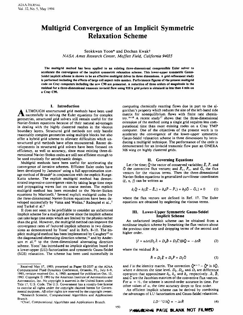
To study the effects of mesh cell aspect ratios on the conver-
gence rates, a low cell aspect ratio 129 x 33 x 33 C-H grid
(140,481 points) is used first. Figure 1 shows the distributionof geometric cell aspect ratios of the first normal mesh cells at
the body from the leading edge to the downstream boundary.
Although geometric aspect ratios are less accurate than spec-
tral radius based aspect ratios, they seem to be useful. The cell
aspect ratios are of the order of 1 at the wing surface. Figure
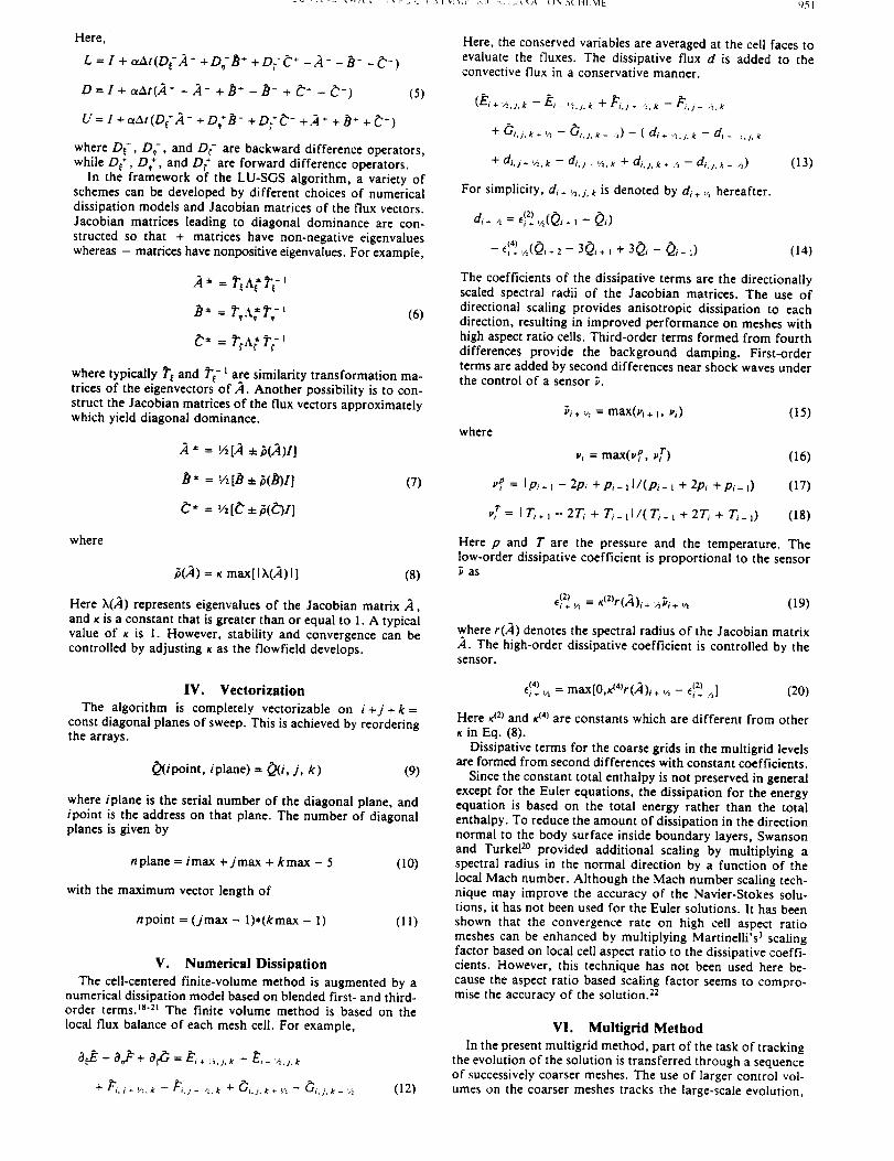
2 shows convergence histories of the root-mean-squared resid-
uals which correspond to the density corrections. The residu-
als are normalized by their initial values. The chained line
indicates the single grid convergence history. The dashed line
indicates the multigrid convergence history using a four-level
V cycle with one iteration on each coarse grid. The solid line
indicates the muitigrid convergence history using a four-level
V cycle with two iterations on each coarse grid. Clearly, the
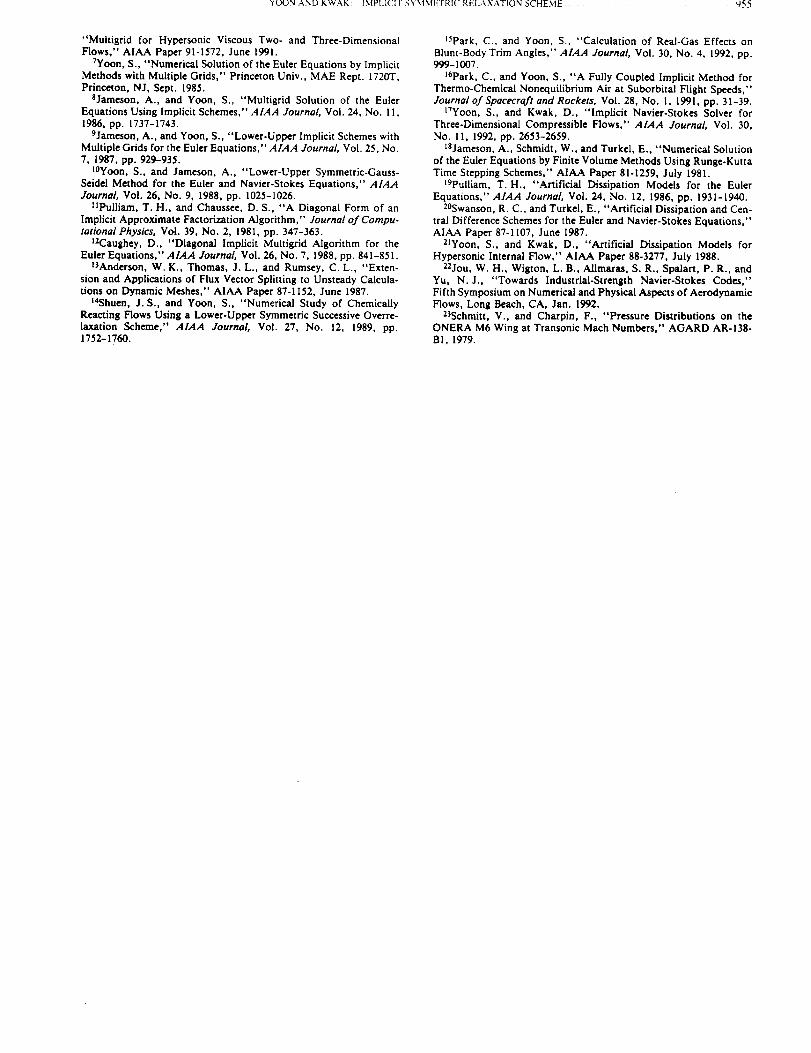
Convergence histories on the fine grid (CPU time on a Cray
fine grid at the 44% semispan station. Single grid convergencehistories are compared in Fig. 6 and show that the convergencerate slows down significantly as the number of grid pointsincreases. Figure 7 shows that multigrid convergence historiesof the three grids are almost identical. Here, the coarse,medium, and fine grids use two-, three-, and four-level Vcycles, respectively. The results demonstrate grid independentconvergence rates which are achieved by the multigrid method.
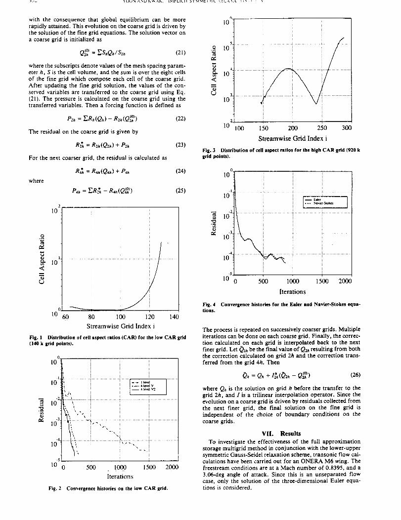
To study the effect of grid stretching on the convergence,another fine grid whose first grid distance is 2.0 x 10 -_ isgenerated. Figure 8 shows that the present numerical methodis insensitive to grid clustering despite the fact that cell aspectratios differ by an order of magnitude. The convergence rateon the highly stretched grid appears to be slightly better thanthe less stretched one for this case. Although not shown here,the rate of convergence slows down significantly after the
Fig. I1C90).
10_
-I
10
lOz
10 .3.
10 .4.
105 0
-J_ '
r
60 120 180 240
CPU min (Cray C90)
Convergence histories on the fine grid (CPU time on a Cray
residual drops about five orders of magnitude on the highlystretched grid.
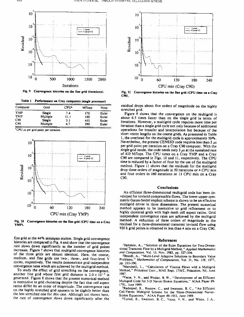
Figure 9 shows that the convergence on the multigrid isabout 6.5 times faster than on the single grid in terms ofiterations. However, a muitigrid cycle requires more time periteration than a single grid cycle not only because of additionaloperations for transfer and interpolation but because of theshort vector lengths on the coarse grids. As presented in Table1, the overhead for the multigrid cycle is approximately 50°70.Nevertheless, the present CENS3D code requires less than 5 _sper grid point per iteration on a Cray C90 computer. With thesingle grid mode, the code needs only 3/_s at the sustained rateof 410 Mflops. The CPU times on a Cray YMP and a CrayC90 are compared in Figs. 10 and l 1, respectively. The CPUtime is reduced by a factor of four by the use of the multigridmethod. Figure 11 shows that the residuals for the multigriddrop three orders of magnitude in 50 iterations or 4 CPU minand four orders in 160 iterations or 13 CPU rain on a CrayC90.
Conclusions
An efficient three-dimensional multigrid code has been de-veloped for inviscid compressible flows. The lower-upper sym-metric Gauss-Seidel implicit scheme is shown to be an effectivemultigrid driver in three dimensions. The present numericalmethod appears to be insensitive to grid refinement or tohighly clustered grids with high mesh cell aspect ratios. Gridindependent convergence rates are achieved by the multigridmethod. A reduction of three orders of magnitude in theresidual for a three-dimensional transonic inviscid flow using920 k grid points is obtained in less than 4 rain on a Cray C90.
References
JJameson, A., "Solution of the Euler Equations for Two-Dimen-
sional Transonic Flow by a Multigrid Method," Applied Mathematics
and Computation, Vol. 13, Nov. 1983, pp. 327-356.
ZBrandt, A., "Multi-Level Adaptive Solutions to Boundary Value
Problems," Mathematics of Computation, Vol. 31, No. 138, 1977,pp. 333-390.
3Martinelli, L., "Calculation of Viscous Flows with a MultigridMethod," Princeton Univ., MAE Rept. 1754T, Princeton, NJ, June1987.
4Vatsa, V. N., and Wedan, B.W., "Development of an EfficientMultigrid Code for 3-D Navier-Stokes Equations," AIAA Paper 89-1791, June 1989.
5Radespiel, R., Rossow, C., and Swanson, R.C., "An EfficientCell-Vertex Multigrid Scheme for the Three-Dimensional Navier-Stokes Equations," AIAA Paper 89-1953, June 1989.
6Turkel, E., Swanson, R.C., Vatsa, V.N., and White, J.A.,
where 7 is the ratio of specific heats. The sound speedis denoted by a. The nondimensional parameters are theReynolds number Re and the Prandtl number Pr. Thecoefficientof viscosity# and thermal conductivityk aredecomposed intolaminar and turbulentcontributionsasfollows:
g = #t _ #t
k - # -( #I #_ )Pr Pr fi'_rl = Pr_
where Pr_ and Prt are the laminar and turbulent Prandttnumbers and k = # with the nondimensionalization used inthis paper. The standard Baldwin-Lomax turbulent eddyviscositymodel [5]ischosenfor thisstudy.
The nondimensionalparameterschosenforthiscode
are the same as thoseinthe CNS code [6].Denoting di-
mensionalquantitieswith a (i,the normalizingparameters
arethe freestreamdensitypoo,thefreestreamsound speedaoc,the freestrea_nviscositycoefficient/_,and a charac-
teristiclengthI.
The metricsused abovehave adifferentmeaning forafinitevolume formulationcompared tothefinitedifference
formulation of [6]. Referring to a typical finite volume cellas shown in figure l, the finite volume metrics are defined(see, for example, Vinokur :rl) a_
s,+z =s -_.,i+ "+s,,÷.;k• .,.. _ sy,_÷ zJ .
1= _[(rr- r2)x (ra- r2)+ (r6- r2)× (r-- r2)]
s_+} = s,.t+½i + %a+½J + s.j_.}k (7)
1= _[(rv- rs)x (r_- rs)+ (re- rs)x (rr- rs)]
The finite volume metrics represent the ce_ face areanormals in each of the curvilinear coordinates (_, V, r).The)" are related to the metrics introduced in equations(1 - 5) as follows
G,V = s,,j+½
,7:,V = s,,,,+½ (S)
_:_V = st,j+ ½
where z, = z,!l,z for i = 1,2,3. The volume of the com-putational cell is given by
1?"= _[(r4- r=) x (rz- rl).(rr- r_)
+(r= - rs) x (re - rl). (rr- re)
+(rs - r4) x (rs- rx)-(rr- rs)] (9)
and isthe finitevolume equivalentof the inverseJacobianof the coordinatetransformationin the finitedifference
formulation of [6].
Numerical Method
The governing equations are integrated in time forboth steady and time accurate calculations. The unfac-tored linear implicit scheme is obtained by lineaxizing theflux vectors about the previous time and dropping secondand higher order terms. The resulting scheme in finitevolume form is given by
A variety of LU-SGS schemes can be obtained by differ-
ent choices of the numerical dissipation models and aaco-
bian matrices of the flux vectors. In this study we use the
same artificial dissipation described for the diagonal Beam-
W'arming scheme. For robustness and to ensure that the
scheme converges to a steady state, the matrices should
be diagonally dominant. To ensure diagonal dominance,the aacobian matrices can be constructed so that 4- ma-
trices have nonnegative eigenvalues and - matrices have
nonpositive eigenvalues. For example, the diagonalization
used for the Beam-Warming scheme can be used to obtainthe m matrices.
._: = T_A_._-_
s= =r,a_T;' (2a)
c_-= z_,ttr;'
Another method to obtain diagonal dominance is to con-struct approximate Jacobian matrices:
A ± = [A ± _(A)I]/2
B ± = [.B ± ,5(B)1"]/2 (24)
c ± =[c ± _(c)z]/2
where _(A) = maz[lA(A)l] and represent a spectral
radius of the Jacobian matrix A with the eigenvalues
A(A). These eigenvalues are, e.g., A(A) = [U, U, U, U ±
_/S S 2 "a _ 4- s_ 4- =].,, where the metric terms are again de-
fined at cell centers by Eq. (19). Other methods ofincrea.s-
ing the diagonal dominance of the LU operator include the
addition some approximation of the viscous terms and the
artificial dissipation in the implicit operator [11].
The inversion of equation (21) is done in three steps.
The block inversionalong the diagonal iseliminated ifthe
approximate Jacobian of Eqn (24) are used instead of Eqn
(23). A Newton-type of iterationisobtained simply by set-
ring h = oo. Eliminating the time step from the algorithm
provides the practicaladvantage of side-steppingthe needto find an optimal CFL number or the time stepscalingto
reduce the overallcomputational effortto achieve steady
state solutions. As mentioned previously, thisis an im-
portant consideration for a multizonal code. Iffirst-order
one-sided differencesare used, Eq. (22) reduces to
L = _3I- A + - B + - C ÷j-l,k,I j,k-1 ,! j,k,l-I
D= _I (25)
U = fir 4- A'_+1,k, t + B_,k+l,t + C_k.t+I
where
= k(A) + _(B)+ _(c)
This algorithm requires only scalar diagonal inversions
since the diagonal of L or U = D. The true Jacobians
matrices of Eq. (23) may permit better convergence rates.
but require block diagonal inversions with approximately
twice the computational effort per iteration. This studyconsiders the scalar version without the viscous or artifi-
cial dissipation only.
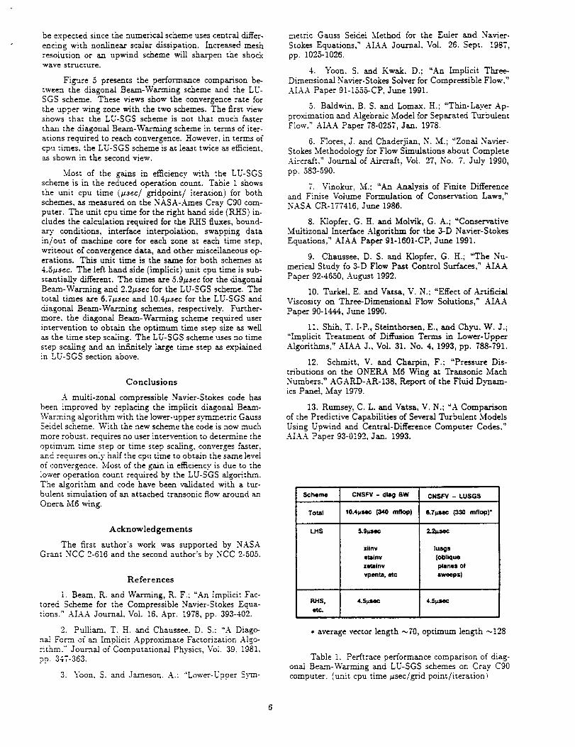
The scheme is completely vectorizable on j 4- k 4- l =
constant oblique planes of sweep, Fig. 2. This can be
achieved by reordering the three dimensional arrays into
two-dimensional arrays as follows:
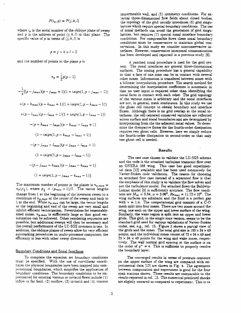
P(ip,p)--P(j,k,l)
where ip is the serial number of the oblique plane of sweepand p is the address of point (j, k.l) in _ha_ plane. Thespecific _lue of p in terms of (J, k, I) is
The maximum number of points in the planes is n,,,_z =
np(p_), where P_t = (P'_: + 1)/2. The vector lengths
change from 1 at the beginning of the inversion sweep to amaximum of np,,_., at the center of the sweep and bare to1 at the end. While np,m.z can be large, the vector lengthsat the beginning and end of the sweep are very small andinhibit efficient vectorization. Neverthelessfor reasonably-sized zones, np,,,,_, is sufficiently large so that good vec-torization can be ar.hieved. Other reordering sequences arepossible, but additional sweeps will then be necessary andthe overall performance of the LU-SGS inversion is less. Inaddition, the oblique planes of sweep allow for very efficientautotasking procedures on multi-processor computers; theefficiency is less with other sweep directions.
Boundary Conditions and Zonal Interfaces
To complete the equation set boundary conditionsmust be specified. With the use of curvillnear coordi-nates the physical boundaries have been mapped into com-putational boundaries, which simplifies the application ofboundary conditions. The boundary, conditions to be im-plemented for external viscous or inviscid flows include (1)inflow or far field. (2) outflow, (3) inviscid and (4) viscous
impermeable wall, and (5) symmetry conditions. For ex-ternal tlxree-dimensional flow fields about closed bodies,the topology of the grid usually introduces (6) grid singu-larities which require special boundary conditions. The useof zonal methods can avoid the generation of grid singu-larities, but requires (7) special zonal interface boundary.conditions. For compressible flows these zonal boundaryconditions must be conservative to maintain global con-servation. In this study we consider nonconservafive in-terfaces. However, conservative interzonal communication
has been developed and reported in a previous study [8].
A patched zonal procedure is used for the grid sys-tem. The zonal interfaces are general three-dimensionalsurfaces. The zoning procedure has a general capabilityso that a face of one zone can be in contact with severalother zones. Information is translated between zones with
a bilinear interpolation procedure. The search method fordetermining the interpolation coefficients is automatic inthat no user input is required other than identifying thezonal faces in contact with each other. The grid topologyof the various zones is arbitrary and the zonal interfacesare not, in general, mesh continuous. In this study we usethe ghost cell concept to obtain boundary, and interfacefluxes. Although there is no grid overlap at the zonal in-terfaces, the ceil-centered conserved variables are reflectedacross surface and zonal boundaries and are determined byinterpolating from the the adjacent zonal values. To deter-mine the dissipative fluxes for the fourth-order dissipationrequires two ghost ceils. However, here we simply reducethe fourth-order dissipation to second-order so that onlyone ghost cell is needed.
Results
The test case chosen to validate the LU-SGS schemeand the code is the attached turbulent transonic flow over
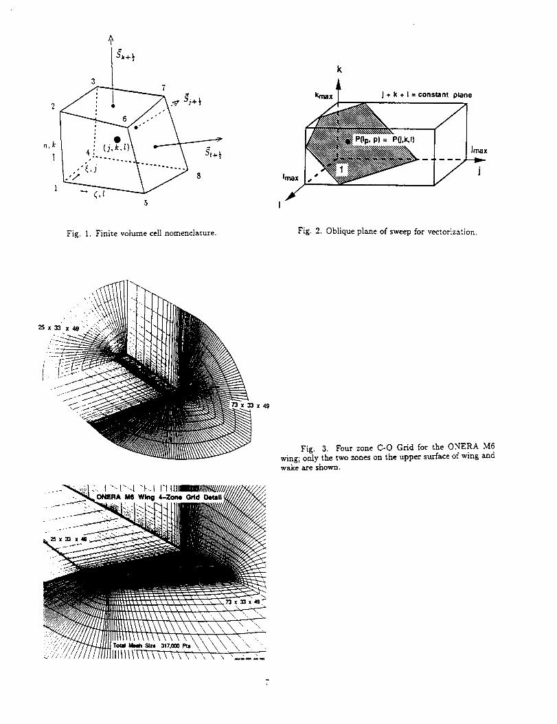
an ONERA M6 wing. This case has good experimen-tal data [12] available and has been used extensively forNavier-Stokes code validation. The reason for choosingan attached flow case instead of a separated flow is thatthe emphasis of this study is to validate the flow solver andnot the turbulence model. For attached flows the Baldwin-Lomax model [3] is sufficiently accurate. The flow condi-tons are M'o_ = 0.84, c_ = 3.06 °, Re,,oc = 11.72 x 10e. Thewing surfaces axe adiabatic and the fluid is a perfect gaswith "y = 1.4. The computational grid consists of a C-Omesh split into four zones. There are two zones around thewing, one each on the upper and lower surface of the wing.Similarly, the wake region is split into an upper and lowergrids. This grid, in the single zone version, seems to be thestandard grid used for various validations of Navier-Stokescodes, see, e.g., ref. 13. Figure 3 shows a partial view ofthe grids and the zones. The total grid size is 193 x 34 x 49points, and the individual zones consist of 73 x 34 x 49 and25 x 34 x 49 points for the wing and wake zones, respec-tively. The wall normal grid spacing at the surface is onthe order of _,+ = 4. This is sufficient to properly resolvethe boundary layer.
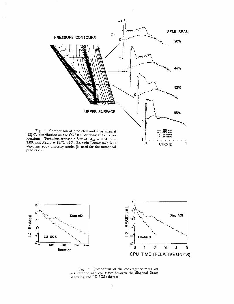
The converged results in terms of pressure contourson the upper surface of the wing are compared with ex-perimental data [12] are shown in Fig. 4. The agreementbetween computation and experiment is good for the fourspan stations shown. These results are comparable to theresults reported in ref. 13. The numerical predicted shocksare slightly smeared as compared to experiment. This is to
be expected since the numerical scheme uses centrnl differ-
encing with nonlinear scalar dissipation. Increased mesh
resolution or an upwind scheme will shaxpen the shock
wave structure.
Figure 5 presents the performance comparison be-
tween the diagonal Bea_n-Warming scheme and the LU-
SGS scheme. These views show the convergence rate for
the upper wing zone with the two schemes. The first viewshows that the LU-SGS scheme is not that much faster
than the diagonal Beam-Waz'ming scheme in terms of iter-
ations required to reach convergence. However, in terms of
cpu times, the LU-SGS scheme is at least twice as efficient,
as shown in the second view.
Most of the gains in efficiency with the LU-SGS
scheme is in the reduced operation count. Table 1 shows
the unit cpu time (_sec/ gridpoint/ iteration) for both
schemes, as measured on the NASA-.,Lmes Cray C90 com-
puter. The unit cpu time for the right hand side (KHS) in-
cludes the calculation required for the KI-IS fluxes, bound-
ary conditions, interface interpolation, swapping data
in/out of machine core for each zone at each time step,
writeout of convergence data, and other miscellaneous op-erations. This unit time is the same for both schemes at
4.5#set. The left hand side (implicit) unit cpu time is sub-
stantinny different. The times are 5.9/asec for the diagonal
Beam-Warming and 2.2/_sec for the LU-SGS scheme. The
total times are 6.7gsec and 10.4#see for the LU-SGS and
more, the diagonal Beam-Warming scheme required user
intervention to obtain the optimum time step size as well
as the time step scaling. The LU-SGS scheme uses no time
step scaling and an infinitely large time step as explainedin LU-SGS section above.
Conclusions
A multi-zonal compressible Navier-Stokes code has
been improved by replacing the implicit diagonal Beam-
Warming algorithm with the lower-upper symmetric GaussSeide[ scheme. With the new scheme the code is now much
more robust, requires no user intervention to determine the
optimum time step or time step scaling, converges faster,and requires only half the cpu time to obtain the same levelof convergence. Most of the gain in efficiency is due to the
lower operation count required by the LU-SGS algorithm.
The algorithm and code have been validated with a tur-bulent simulation of an attached transonic flow around an
Onera M6 wing.
Acknowledgements
The first author's work was supported by NASA
Grant NCC 2-61(5 and the second author's by NCC 2-505.
References
1. Beam, R. and Warming, K. F.; "An Implicit Fac-
tored Scheme for the Compressible Navier-Stokes Equa-
tions." AIAA Journal, VoI. 16, Apr. 1978, pp. 393-402.
2. Pulliam. T. H. and Chaussee. D. S.: "A Diago-
nal Form of an Implicit Approximate Factorization Algo-
rithm." Journal of Computational Physics, Voi. 39, 1981,
pp. 34:-363.
3. Yoon. S. and Jameson. A.: "Lower-Upper Sym-
metric Gauss Seidet Method for the Euler and Navier-