Convection Heat Transfer Reading Problems 19-1 → 19-8 19-15, 19-24, 19-35, 19-47, 19-53, 19-69, 19-77 20-1 → 20-6 20-21, 20-28, 20-44, 20-57, 20-79 Introduction • in convective heat transfer, the bulk fluid motion of the fluid plays a major role in the over- all energy transfer process. Therefore, knowledge of the velocity distribution near a solid surface is essential. • the controlling equation for convection is Newton’s Law of Cooling ˙ Q conv = ΔT R conv = hA(T w − T ∞ ) ⇒ R conv = 1 hA where A = total convective area,m 2 1
• in convective heat transfer, the bulk fluid motion of the fluid plays a major role in the over-all energy transfer process. Therefore, knowledge of the velocity distribution near a solidsurface is essential.
• the controlling equation for convection is Newton’s Law of Cooling
Qconv =ΔT
Rconv
= hA(Tw − T∞) ⇒ Rconv =1
hA
where
A = total convective area, m2
1
h = heat transfer coefficient, W/(m2 · K)
Tw = surface temperature, ◦C
T∞ = fluid temperature, ◦C
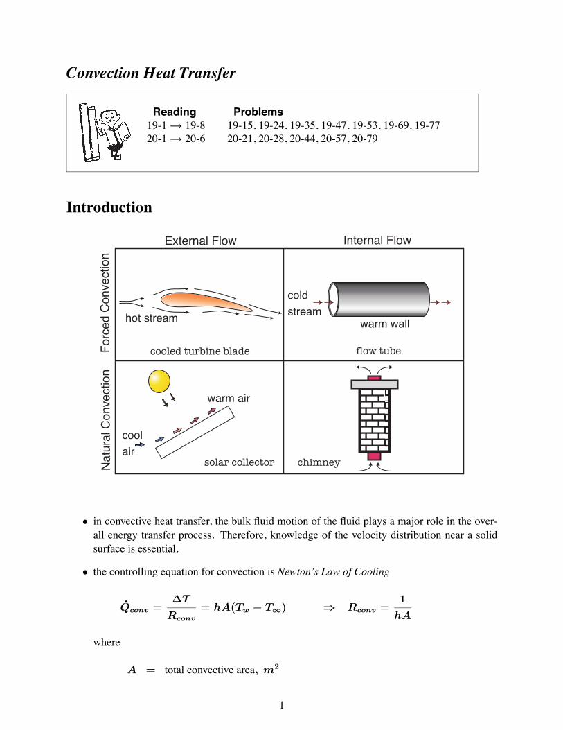
External Flow: the flow engulfs the body with which it interacts thermally
Internal Flow: the heat transfer surface surrounds and guides the convective stream
Forced Convection: flow is induced by an external source such as a pump, compressor, fan, etc.
Natural Convection: flow is induced by natural means without the assistance of an externalmechanism. The flow is initiated by a change in the density of fluids incurred as a resultof heating.
Mixed Convection: combined forced and natural convection
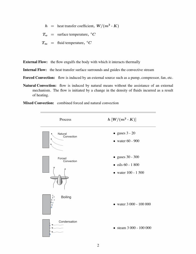
Process h [W/(m2 · K)]
NaturalConvection
• gases 3 - 20
• water 60 - 900
ForcedConvection
• gases 30 - 300
• oils 60 - 1 800
• water 100 - 1 500
Boiling
• water 3 000 - 100 000
Condensation
• steam 3 000 - 100 000
2
Dimensionless GroupsPrandtl number: Pr = ν/α where 0 < Pr < ∞ (Pr → 0 for liquid metals and Pr →
∞ for viscous oils). A measure of ratio between the diffusion of momentum to the diffusionof heat.
Reynolds number: Re = ρUL/μ ≡ UL/ν (forced convection). A measure of the balancebetween the inertial forces and the viscous forces.
Peclet number: Pe = UL/α ≡ RePr
Grashof number: Gr = gβ(Tw − Tf)L3/ν2 (natural convection)
Nusselt number: Nu = hL/kf This can be considered as the dimensionless heat transfercoefficient.
Stanton number: St = h/(UρCp) ≡ Nu/(RePr)
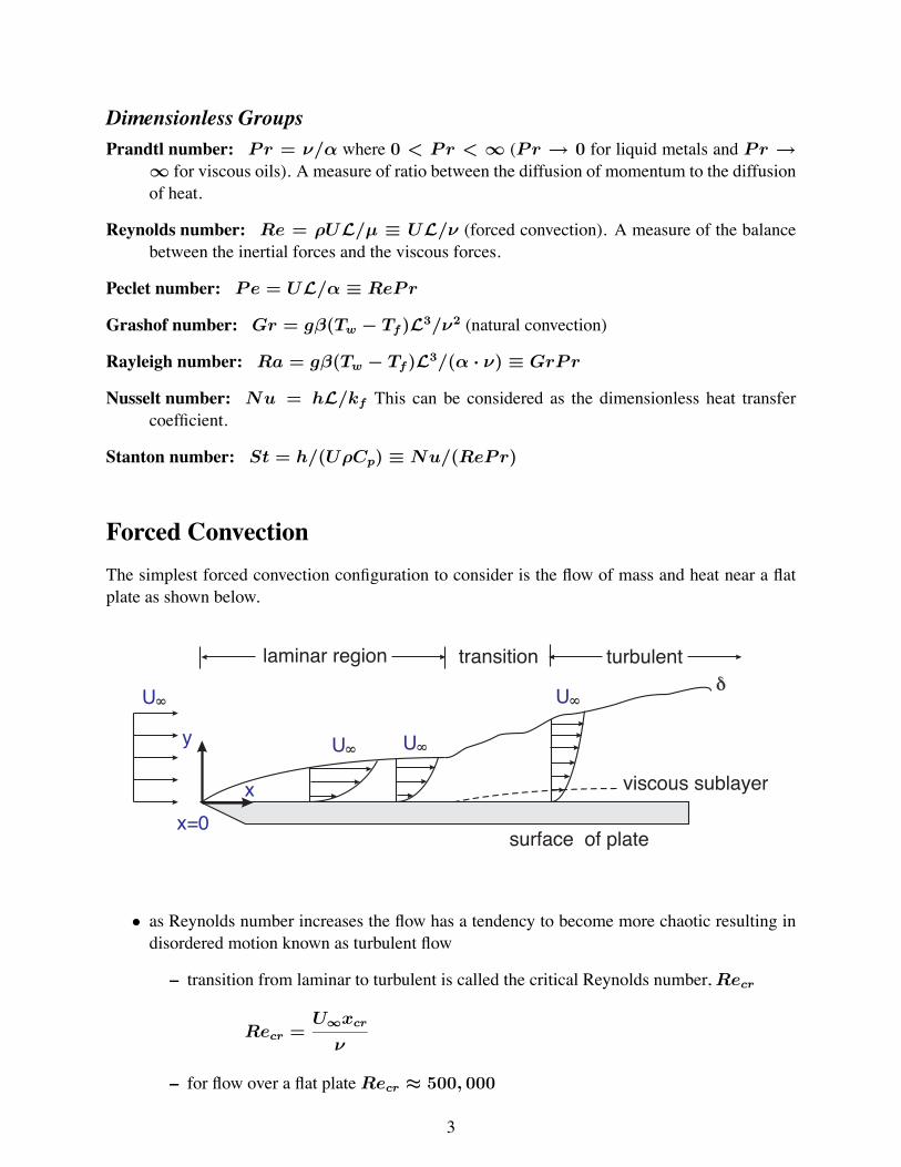
Forced Convection
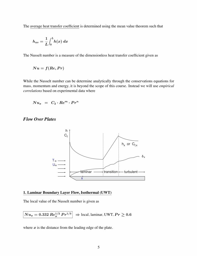
The simplest forced convection configuration to consider is the flow of mass and heat near a flatplate as shown below.
• as Reynolds number increases the flow has a tendency to become more chaotic resulting indisordered motion known as turbulent flow
– transition from laminar to turbulent is called the critical Reynolds number, Recr
Recr =U∞xcr
ν
– for flow over a flat plate Recr ≈ 500, 000
3
– for engineering calculations, the transition region is usually neglected, so that the tran-sition from laminar to turbulent flow occurs at a critical location from the leading edge,xcr
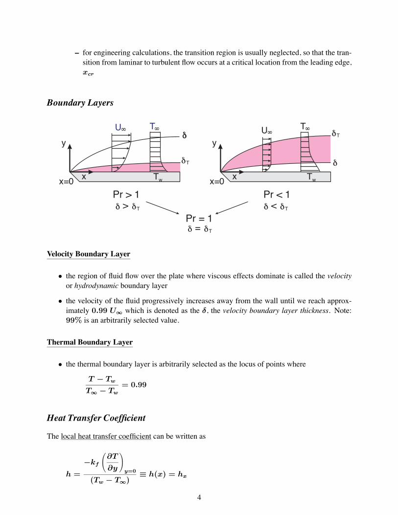
Boundary Layers
Velocity Boundary Layer
• the region of fluid flow over the plate where viscous effects dominate is called the velocityor hydrodynamic boundary layer
• the velocity of the fluid progressively increases away from the wall until we reach approx-imately 0.99 U∞ which is denoted as the δ, the velocity boundary layer thickness. Note:99% is an arbitrarily selected value.
Thermal Boundary Layer
• the thermal boundary layer is arbitrarily selected as the locus of points where
T − Tw
T∞ − Tw
= 0.99
Heat Transfer Coefficient
The local heat transfer coefficient can be written as
h =
−kf
(∂T
∂y
)y=0
(Tw − T∞)≡ h(x) = hx
4
The average heat transfer coefficient is determined using the mean value theorem such that
hav =1
L
∫ L
0h(x) dx
The Nusselt number is a measure of the dimensionless heat transfer coefficient given as
Nu = f(Re, Pr)
While the Nusselt number can be determine analytically through the conservations equations formass, momentum and energy, it is beyond the scope of this course. Instead we will use empiricalcorrelations based on experimental data where
1. Boundary Layer Flow Over Circular Cylinders, Isothermal (UWT)
The Churchill-Berstein (1977) correlation for the average Nusselt number for long (L/D > 100)cylinders is
NuD = S∗D + f(Pr) Re
1/2D
⎡⎣1 +
(ReD
282000
)5/8⎤⎦4/5
⇒average, UWT, Re < 107
0 ≤ Pr ≤ ∞, Re · Pr > 0.2
where S∗D = 0.3 is the diffusive term associated with ReD → 0 and the Prandtl number function
is
f(Pr) =0.62 Pr1/3
[1 + (0.4/Pr)2/3]1/4
All fluid properties are evaluated at Tf = (Tw + T∞)/2.
2. Boundary Layer Flow Over Non-Circular Cylinders, Isothermal (UWT)
The empirical formulations of Zhukauskas and Jakob are commonly used, where
NuD ≈ hD
k= C Rem
D Pr1/3 ⇒ see Table 19-2 for conditions
3. Boundary Layer Flow Over a Sphere, Isothermal (UWT)
For flow over an isothermal sphere of diameter D
NuD = S∗D +
[0.4 Re
1/2D + 0.06 Re
2/3D
]Pr0.4
(μ∞
μw
)1/4
⇒
average, UWT,
0.7 ≤ Pr ≤ 380
3.5 < ReD < 80, 000
where the diffusive term at ReD → 0 is S∗D = 2
and the dynamic viscosity of the fluid in the bulk flow, μ∞ is based on T∞ and the dynamicviscosity of the fluid at the surface, μw, is based on Tw. All other properties are based on T∞.
7
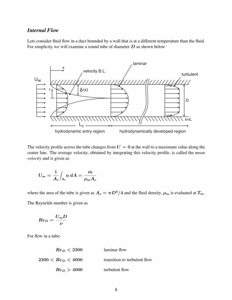
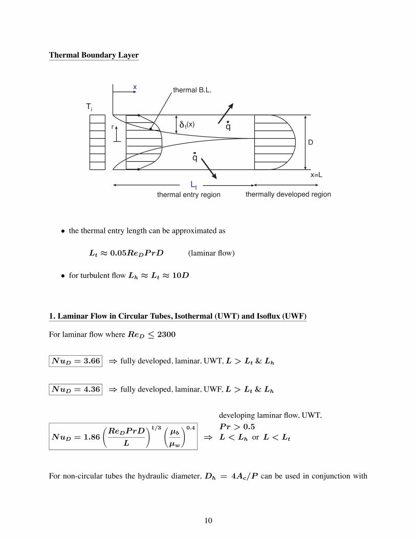
Internal Flow
Lets consider fluid flow in a duct bounded by a wall that is at a different temperature than the fluid.For simplicity we will examine a round tube of diameter D as shown below
The velocity profile across the tube changes from U = 0 at the wall to a maximum value along thecenter line. The average velocity, obtained by integrating this velocity profile, is called the meanvelocity and is given as
Um =1
Ac
∫Ac
u dA =m
ρmAc
where the area of the tube is given as Ac = πD2/4 and the fluid density, ρm is evaluated at Tm.
The Reynolds number is given as
ReD =UmD
ν
For flow in a tube:
ReD < 2300 laminar flow
2300 < ReD < 4000 transition to turbulent flow
ReD > 4000 turbulent flow
8
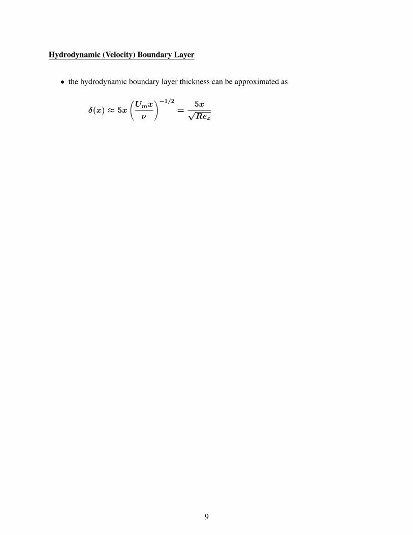
Hydrodynamic (Velocity) Boundary Layer
• the hydrodynamic boundary layer thickness can be approximated as
δ(x) ≈ 5x
(Umx
ν
)−1/2
=5x√Rex
9
Thermal Boundary Layer
• the thermal entry length can be approximated as
Lt ≈ 0.05ReDPrD (laminar flow)
• for turbulent flow Lh ≈ Lt ≈ 10D
1. Laminar Flow in Circular Tubes, Isothermal (UWT) and Isoflux (UWF)
For non-circular tubes the hydraulic diameter, Dh = 4Ac/P can be used in conjunction with
10
Table 10-4 to determine the Reynolds number and in turn the Nusselt number.
In all cases the fluid properties are evaluated at the mean fluid temperature given as
Tmean =1
2(Tm,in + Tm,out)
except for μw which is evaluated at the wall temperature, Tw.
2. Turbulent Flow in Circular Tubes, Isothermal (UWT) and Isoflux (UWF)
For turbulent flow where ReD ≥ 2300 the Dittus-Bouler equation (Eq. 19-79) can be used
NuD = 0.023 Re0.8D Prn ⇒
turbulent flow, UWT or UWF,0.7 ≤ Pr ≤ 160
ReD > 2, 300
n = 0.4 heating
n = 0.3 cooling
For non-circular tubes, again we can use the hydraulic diameter, Dh = 4Ac/P to determine boththe Reynolds and the Nusselt numbers.
In all cases the fluid properties are evaluated at the mean fluid temperature given as
Tmean =1
2(Tm,in + Tm,out)
11
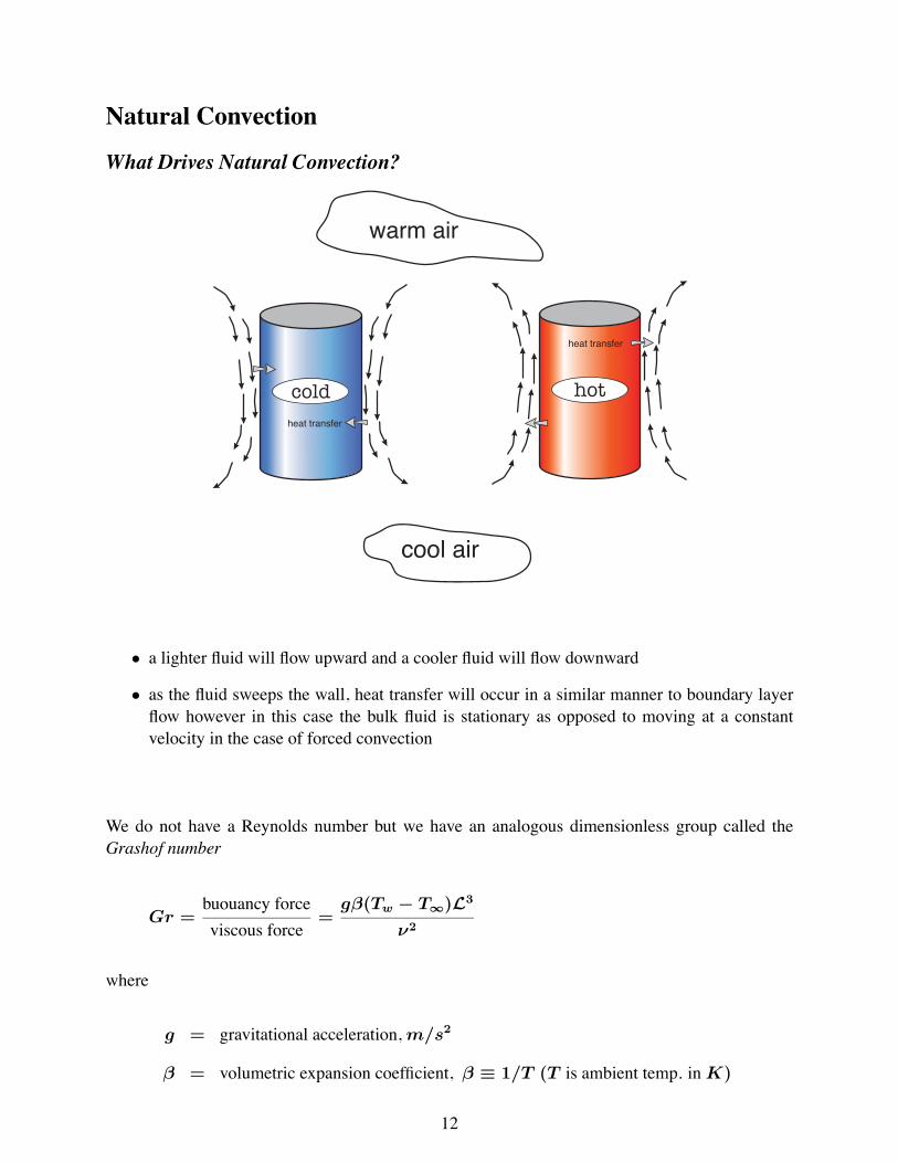
Natural Convection
What Drives Natural Convection?
• a lighter fluid will flow upward and a cooler fluid will flow downward
• as the fluid sweeps the wall, heat transfer will occur in a similar manner to boundary layerflow however in this case the bulk fluid is stationary as opposed to moving at a constantvelocity in the case of forced convection
We do not have a Reynolds number but we have an analogous dimensionless group called theGrashof number
Gr =buouancy force
viscous force=
gβ(Tw − T∞)L3
ν2
where
g = gravitational acceleration, m/s2
β = volumetric expansion coefficient, β ≡ 1/T (T is ambient temp. in K)
12
Tw = wall temperature, K
T∞ = ambient temperature, K
L = characteristic length, m
ν = kinematic viscosity, m2/s
The volumetric expansion coefficient, β, is used to express the variation of density of the fluid withrespect to temperature and is given as
β = −1
ρ
(∂ρ
∂T
)P
Natural Convection Heat Transfer Correlations
The general form of the Nusselt number for natural convection is as follows:
Nu = f(Gr, Pr) ≡ CRamPrn where Ra = Gr · Pr
• C depends on geometry, orientation, type of flow, boundary conditions and choice of char-acteristic length.
• m depends on type of flow (laminar or turbulent)
• n depends on the type of fluid and type of flow
1. Laminar Flow Over a Vertical Plate, Isothermal (UWT)
The general form of the Nusselt number is given as
NuL =hLkf
= C
⎛⎜⎜⎜⎝gβ(Tw − T∞)L3
ν2︸ ︷︷ ︸≡Gr
⎞⎟⎟⎟⎠
1/4 ⎛⎜⎜⎜⎝ ν
α︸︷︷︸≡P r
⎞⎟⎟⎟⎠
1/4
= C Gr1/4L Pr1/4︸ ︷︷ ︸Ra1/4
where
RaL = GrLPr =gβ(Tw − T∞)L3
αν
13
2. Laminar Flow Over a Long Horizontal Circular Cylinder, Isothermal (UWT)
The general boundary layer correlation is
NuD =hD
kf
= C
⎛⎜⎜⎜⎝gβ(Tw − T∞)D3
ν2︸ ︷︷ ︸≡Gr
⎞⎟⎟⎟⎠
n ⎛⎜⎜⎜⎝ ν
α︸︷︷︸≡P r
⎞⎟⎟⎟⎠
n
= C GrnD Prn︸ ︷︷ ︸Ran
D
where
RaD = GrDPr =gβ(Tw − T∞)D3
αν
All fluid properties are evaluated at the film temperature, Tf = (Tw + T∞)/2.
14
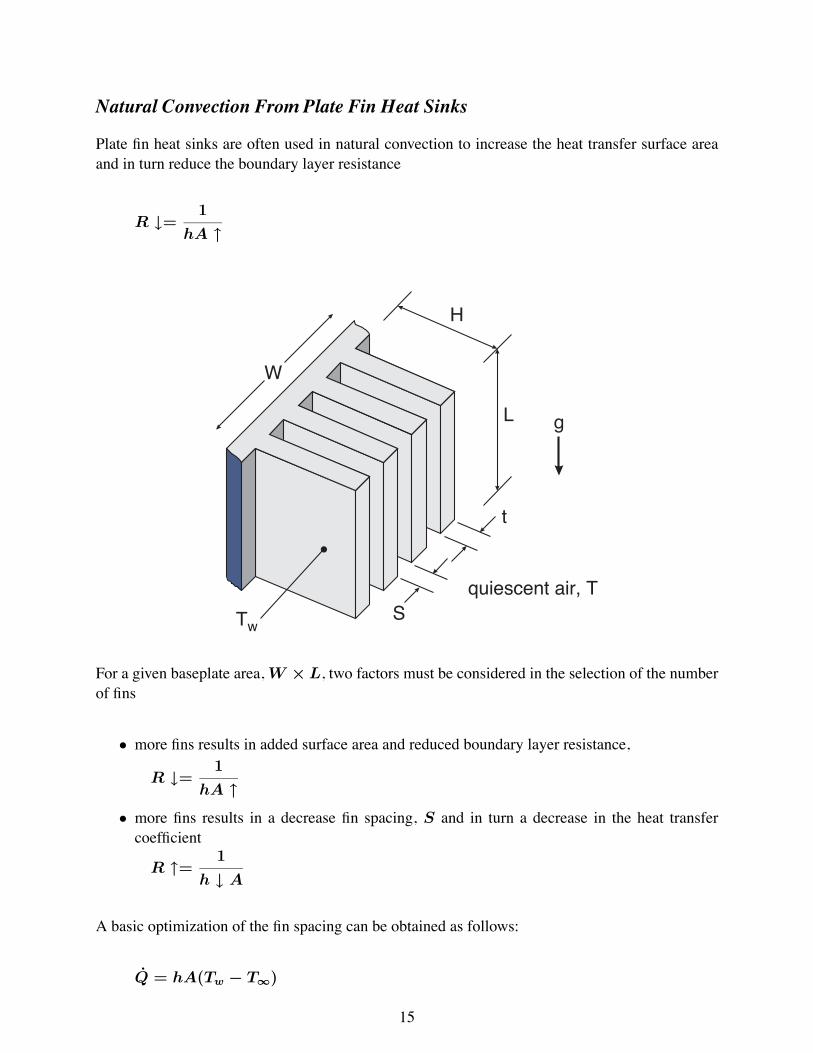
Natural Convection From Plate Fin Heat Sinks
Plate fin heat sinks are often used in natural convection to increase the heat transfer surface areaand in turn reduce the boundary layer resistance
R ↓=1
hA ↑
For a given baseplate area, W × L, two factors must be considered in the selection of the numberof fins
• more fins results in added surface area and reduced boundary layer resistance,
R ↓=1
hA ↑• more fins results in a decrease fin spacing, S and in turn a decrease in the heat transfer
coefficient
R ↑=1
h ↓ A
A basic optimization of the fin spacing can be obtained as follows:
Q = hA(Tw − T∞)
15
where the fins are assumed to be isothermal and the surface area is 2nHL, with the area of the finedges ignored.
For isothermal fins with t < S
Sopt = 2.714
(L
Ra1/4
)
with
Ra =gβ(Tw − T∞L3)
ν2Pr
The corresponding value of the heat transfer coefficient is
h = 1.31k/Sopt
All fluid properties are evaluated at the film temperature.
![International Journal of Heat and Mass Transfergaguilar/PUBLICATIONS/Lorenzos/Transient lamina… · Yao [8] obtained an analytical solution for the fluid flow and the heat transfer](https://static.documents.pub/doc/80x56/5b3c38337f8b9a26728d3c81/international-journal-of-heat-and-mass-gaguilarpublicationslorenzostransient.jpg)


