Coordinated Model Predictive Control of Aircraft Gas TurbineEngine and Power System
Jinwoo Seok,∗ Ilya Kolmanovsky,† and Anouck Girard‡
University of Michigan, Ann Arbor, Michigan 48109-2140
DOI: 10.2514/1.G002562
Motivated by the growing need to accommodate large transient thrust and electrical load requests in future
more-electric aircraft, a coordinated control strategy for a gas turbine engine, generators, and energy storage is
developed. An advanced two-generator configuration, with each generator connected to a shaft of the gas turbine
engine, is treated. Model predictive control maximizes system performance and protects this system against
constraint violations. The controller design is exploits rate-based linear prediction models. In addition, an auxiliary
offset state improves the match between the linear prediction model and the nonlinear system. The auxiliary offset
state allows the system to be controlled over the large operating range without requiring multiple linearizations/
controllers. The advantages of different energy storages are also compared to complement the two-generator
configuration in a more electric aircraft. Primary results indicate that the coordinated model predictive control with
an auxiliary offset state yields better performance than other control strategies, and it successfully controls the
considered system to satisfy specified requirements over a large operating range. The battery–ultracapacitor pack
allows improvement of the overall system performance.
I. Introduction
I N THE past few decades, the electrical power requirements foraircraft have been steadily increasing, and this growth has been
concomitant with trends towardmore-electric aircraft (MEA) and all-electric aircraft (AEA) [1]. A typical aircraft power system involvesone or more generators connected to one or more gas turbine engines,
which are integrated with energy storage elements that providesupplemental electrical power, a distribution system, and loads. Thelarge electrical loads, including both steady and transient loads, affectthe operation of the generators and of the gas turbine engines. For
instance, large electrical load changes induce large torquedisturbances on the gas turbine engine and can affect engine thrustand shaft speeds. These changes, in turn, affect the generators; hence,
the system exhibits strong static and dynamic interactions. Thus, inthe presence of large electrical loads, the interactions between theelectrical system and the gas turbine engine have to be addressed forthe efficient and safe operation of aircraft.Our objective is to establish an integrated model-based control
capability for an aircraft’s propulsion and electrical power systems
(including thrust generation, electric power generation, and energystorage) that improves the capability of the system to accommodatelarge transients, including those caused by large transient electrical
loads, while maintaining the operation of the components andthe overall system within a specified safe range by enforcingappropriately defined state and control constraints.Specifically, this paper considers the development of an integrated
control system that accommodates large steady and transient
electrical loads; maintains aircraft flight performance by deliveringrequested thrust; enforces gas turbine engine constraints (e.g., surgemargins), as well as electrical system constraints (e.g., componentpower limits); and reduces fuel consumption. To facilitate the
achievement of these goals, an advanced two-shaft distributed
generator configuration is considered, where one generator isconnected to the high-pressure shaft (HPS) and the other is connectedto the low-pressure shaft (LPS) of the gas turbine engine. Thisconfiguration affords an extra degree of freedom to accommodate theeffects of large loads compared to the single-shaft configuration.Furthermore, it potentially achieves better fuel efficiency than thesingle-shaft configuration. In addition, the integration of high-performance storage elements that can react quickly to transient loadsto assist the generators and the gas turbine engines is considered.To control such an advanced system with two generators, a gas
turbine engine, and energy storage, we define a power split strategybetween the two generators based on the offline minimization of thefuel consumption and a rule-based strategy to determine when tocharge and discharge the energy storage. To protect the engine and theelectrical system components against constraint violation, a rate-based model predictive control (MPC) framework is exploited andseveral MPC controller designs are developed, validated on anonlinear model of the system, and compared with each other. Theproposed framework is flexible and modular, and it can accommodateother constraints not explicitly treated in the paper, such as temperatureconstraints in the engine or voltage stability constraints in the electricalsystem, provided the prediction model is updated with representationsfor these constraints. Because only linear MPC design techniques areemployed, the controller implementation is feasible with standardquadratic programming solvers, which are a mature and reliabletechnology.The system configuration of interest in this paper is illustrated in
Fig. 1. The system consists of a single gas turbine engine, energystorage element(s), and two generators: one of which is attached tothe LPS of the gas turbine engine, whereas the other is attached to theHPS of the gas turbine engine.The growing electrical power requirements of MEA and AEA are
highlighted in [1,2]. For instance, at least 1.6MWwill be required fora next-generation 300-passenger aircraft [2]. Large electrical poweris required for turboelectric propulsion. Three megawatt generatorswere considered in [3], and a 40.2 MW generator was planned in[4,5]. Electrical weapons systems for military applications alsorequire large electrical power: from 0.025 to 4.5 MW, depending onthe type [6]. Directed energy systems are one of the key 12 potentialcapability areas for the U.S. Air Force [7]. To deal with these largeelectrical loads on aircraft, integrated control of the aircraft’s gasturbine engine, electrical power system, and thermal management isnecessary. Challenges in aircraft engine control and integrated powerand thermal management were discussed in [8–11].MPC-based approaches have been considered to develop solutions
to many recent control problems, including gas turbine engine
control; see, e.g., [12–14]. Rate-based MPC allows setpoint trackingand was applied to turbofan engine clearance control in [13] and toturbocharged compression ignition engine control in [15]. In thispaper, the Multi-Parametric Toolbox (MPT) [16] is employed forcomputational implementation of a rate-based MPC controller.The two-generator configuration for aircraft, with one generator
connected to theHPS and the other generator connected to the LPS ofa gas turbine engine, was introduced in [17]. The challenges andpossible research directions for unmanned aerial vehicles and MEAwith a gas turbine engine, a two-generator configuration, and abattery (and/or supercapacitor) were discussed in [18]. The authors of[18] indicated the necessity of integrated control of the electricalsystem and the gas turbine engine due to interactions between bothsystems. In [19], the authors designed a voltage and current controllerfor the generators, and this work was extended in [20]to include a battery. The controller proposed in these referenceswas based on a master–slave configuration for high-load situations.Existing publications on two-generator configurations focusedprimarily on the electrical system, especially voltage and currentstability, and a control design exploiting batteries.Integrated control of a gas turbine engine and electrical power
system has been considered in some publications. The nonlinearMPC approach for a 166 MW heavy-duty single-shaft gas turbinepowerplant based on simplified gas turbine engine and generatormodels was presented in [21]. The control goal was to supply all-electrical loads while maintaining the rotor speed, exhaust gastemperature, and turbine firing temperature by controlling airflowand fuel flow despite transient load changes. The control of thegas turbine engine and electrical system, which focused on theirthermal management, for the U.S. Navy’s future all-electric ship wasconsidered in [22]. The importance of interactions between the gasturbine engine and the electrical system for aircraft was highlighted in[23], where the engine response when a step change reduction ofelectrical power occurred was simulated. In [24], an energy storageelement (supercapacitor)wasused to reduce the effects of dynamic loadson the engine using a proportional-integral (PI) supercapacitorcontroller. A load management system, which consisted of generators,contactors, buses, loads, and a battery for an aircraft electric powersystem was presented in [25]. The paper [25] focused on the electricalsystem of the aircraft, mainly controlling contactors for safety andreliability, using load shedding.The aircraft gas turbine enginemodelingand control were discussed in [26].In this paper, the following problem formulation is considered:
Given a gas turbine engine; energy storage elements; two generators,with one connected to each shaft of the gas turbine engine; arequested thrust level; and (large) expected/requested electricalloads, determine the fuel-to-air ratio of the gas turbine engine,
the input/output power of the energy storage elements, and theelectrical power output of each generator to supply all the requiredelectrical loads, maintain the requested thrust level, and minimize fuelconsumption, subject to surge margin limits and other constraints.The Simulink-based Toolbox for the Modeling and Analysis of
Thermodynamic Systems (T-MATS) [27–29] is used for the gasturbine engine modeling and is supplemented by an electrical powersystemmodel in Simulink. T-MATSallows one tomodel both steady-state and dynamic gas turbine engine operation.The original contributions of this paper are now highlighted. Most
of the existing studies on the two-generator configuration are limitedonly to the electrical system. In this paper, the effects on the gasturbine engine are considered, and it is shown that coordinatedcontrol solutions can be developed to increase capability andefficiency of the system. An advanced electrical power systemconfigurationwith two generators and an electrical storage element isalso treated, for which control designs based on MPC are developedthat accomplish simultaneous tracking of requested thrust andelectrical power output commands while satisfying the imposedcomponent protection constraints within the engine and the electricalsystem, as well as minimizing fuel consumption. These designsaccount for static and dynamic interactions between the gas turbineengine, generators, and energy storage. The paper illuminates the linkbetween energy storage characteristics and control performance.Existing aircraft power systems are typically optimized on a quasi-
static individual component basis. Here, a novel control systemarchitecture based on the combination of a rate-based linear quadratic/MPC controller, a power split map between generators optimizedfor steady-state operation, and a supervisory logic to govern energystorage charging/discharging is defined. The benefits of constrainedcoordinated control include the ability to handle load pulses of higherfrequency and a larger magnitude than possiblewith existing systems.Unlike many of the previous publications, system operation over
a large static and dynamic range is considered in this paper. TheMPC controller designs based on single linear and multiple linearprediction models are compared where the linear prediction modelsare obtained by applying system identification techniques. As thepaper shows, the mismatch between the linear prediction models andthe actual nonlinear system can be successfully handled by auxiliaryoffset states; in particular, the surge margin constraints can berobustly enforced. A novel linear transformation approach to matchstates of different linear prediction models is also proposed. Thisapproach avoids the need for designing observers for nonphysicalstates of the individual models. Furthermore, the paper demonstratesthat successful control of the system can be accomplished by usinga single rate-based linear prediction model with lower computationaland implementational complexity as compared to the switched MPC
Fig. 1 Schematic of the gas turbine engine and the electrical power system.
SEOK, KOLMANOVSKY, AND GIRARD 2539
Dow
nloa
ded
by U
NIV
ER
SIT
Y O
F M
ICH
IGA
N o
n A
pril
5, 2
018
| http
://ar
c.ai
aa.o
rg |
DO
I: 1
0.25
14/1
.G00
2562
approach. Based on a comparison of the closed-loop response withthe one from the classical linear quadratic regulator (LQR) controller,the advantages of MPC are highlighted. We validate the design innonlinear model simulations over the large engine operating rangewhile responding to large transient thrust and electrical power loadcommands. As considered case studies demonstrate, the MPCcontrol design framework is systematic and expandable to includeadditional components.This work extends and goes much beyond our previous work that
appeared in a conference paper [30]. In particular, in this paper, thesystem configuration with the energy storage elements is treated, thepower split strategy for the tradeoff between the fuel consumptionand the surgemargin (rather than just fuel consumption) is optimized,and MPC controllers for the large operating range of the engineare developed and demonstrated to accommodate simultaneoustransients in electrical load and thrust. The rate-based MPC designsbased on a single andmultiple linear models are compared, and offsetstates are introduced to compensate for the differences in responsebetween the linear model and the nonlinear system. The lineartransformation of the linear models is also introduced to match thestates of the multiple linear models with the physical states.The organization of this paper is as follows. Section II describes the
system models and how linear models are constructed to predictsystem response. Section III addresses the control design. Section IVpresents the simulation results on the full nonlinear model. Finally,Sec. V presents our conclusions.
II. Modeling
In this section, models of the gas turbine engine, generators, andenergy storage elements are described. A simple relationshipbetween the shaft speeds of the gas turbine engine and the outputpower of the generators is used, assuming the dynamics of thegenerators are much faster than the dynamics of the gas turbineengine; and a first-order model is adopted to represent the dynamicsof the energy storage elements. The engine model, generator models,and energy storage element models are assembled into a system levelmodel in which one generator is connected to the HPS and the othergenerator is connected to the LPS of the gas turbine engine. Note thatthe assembledmodel is able to represent subsystem-level interactionsvisible in the simulation results.Then, a linearmodel of the gas turbine enginewith two generators is
obtained via system identification, followed by a linear transformationof all the states of the linear model to physical states. Note that theidentified linear model takes into account the interactions between thegas turbine engine and the generators. Finally, the identified linearmodel, the generator models, and the energy storage element modelsare combined to obtain the complete linear predictionmodel to be usedin MPC control design.
A. Gas Turbine Engine
The JT9D gas turbine engine model provided with the T-MATSpackage [28] is used to represent engine dynamics. T-MATS is aSimulink-based tool for thermodynamic system simulation that wasdeveloped and released by NASA to facilitate research involving gasturbine engine simulations and control of the kind pursued in thispaper. Unlike other packages, T-MATS is open to public use. Itincludes generic modeling libraries and is suitable for gas turbineengine modeling. The JT9D gas turbine engine model represents thedynamics of shaft speeds, pressures, and flows invarious componentsof the engine and predicts engine thrust. The model is developed andverified based on data from the numerical propulsion systemsimulation [29]. The thrust Fg is controlled using the fuel-to-air ratio(FAR) as a control input.
B. Generators
The two generators are each connected to different shafts of the gasturbine engine: one to the HPS, and one to the LPS. We refer to thegenerator that is connected to the HPS as the high-pressure shaftgenerator (HPSG) and the generator that is connected to the LPS as
the low-pressure shaft generator (LPSG). Then, the power requestedfrom the HPSG PHreq and the power requested from the LPSG PLreq
are two additional control inputs in our system. The total outputpower from the generatorsPGT
is the sum of the output powers of theHPSG PH and LPSG PL. The power difference between twogenerators PD is one of the outputs of the system and is definedas PH − PL.Assuming that the dynamics of the generators are much faster than
those of the gas turbine engine [31], a simple relationship between theshaft speeds of the gas turbine engine and the output power of thegenerators is adopted based on given efficiencies of the generators:
PH � NH × τEH× ηH;
PL � NL × τEL× ηL (1)
whereNH , τEH, and ηH are, respectively, the shaft speed, the torque on
the shaft, and the efficiency of the HPSG; and NL, τEL, and ηL are,
respectively, the shaft speed, the torque on the shaft, and theefficiency of the LPSG. Thus, given electrical power outputs of thegenerators, the torques that the generators create on the gas turbineengine shafts can be computed according to
τEH� PH
NH × ηH;
τEL� PL
NL × ηL(2)
Note that the preceding electrical power system representation issuitablewhen given the specific control objectives in this paper, and itis justified by the timescale separation between the engine dynamicsand the dynamics in the electrical power system. In the subsequentanalysis and simulations, constant values of the efficiencies(ηH � ηL � 0.9) are assumed.
C. Energy Storage Elements
The energy storage element model is as follows:
dEj
dt� −Pj (3)
whereEj is the total energy stored in the energy storage j,Pj is powerto/from the energy storage j, and j indicates the type of energystorage element. In this paper, a battery and/or ultracapacitor areexploited as the energy storage elements, so j ∈ fB;Cg, where Bindicates the battery andC indicates the ultracapacitor. Then, the stateof charge (SOC) is given by
SOCj �Ej
EjMax
(4)
where EjMaxis the maximum energy that can be stored in the energy
storage j. The total output/input power of the energy storage elementsPEST
is the sum of the output/input power of all the energy storageelements. Then, the total output power PT is the sum of the totaloutput powers from the generators PGT
and the total output/inputpowers of the energy storage elements PEST
.
D. Linear Design Model
1. System Identification and Linear Transformation
The design of our MPC controller is based on a linear predictionmodel. Because our gas turbine engine model is essentially of theblack-box type, either analytical or numerical (finite difference-based) linearization cannot be easily implemented. Consequently, thelinear model is identified based on the input–output response datacollected from the nonlinear model of the engine near a nominaloperating point. The nominal operating point is the same as the oneused for verifying the model in [29] (27,593 lbf thrust and FAR of0.0187), and PHreq � PLreq � 0 MW.Our linear model to be identified has three inputs (FAR,PHreq, and
PLreq) and five outputs [HPS speed, LPS speed, thrust, low-pressure
2540 SEOK, KOLMANOVSKY, AND GIRARD
Dow
nloa
ded
by U
NIV
ER
SIT
Y O
F M
ICH
IGA
N o
n A
pril
5, 2
018
| http
://ar
c.ai
aa.o
rg |
DO
I: 1
0.25
14/1
.G00
2562
compressor (LPC) surge margin, and high-pressure compressor(HPC) surge margin. The surge margins are added as outputs to the
model to predict the evolution of the surgemargin constraints over theprediction horizon.To identify the linear predictionmodel at a given operating point, a
system identification approach is followed. The input–output dataset
is based on a 400 s trace generated when chirp signals are applied toeach of FAR, PHreq, and PLreq channels for 100 s individually; andthen it is applied to all inputs in combination for another 100 s. The
magnitude of chirp signals is set to 0.001 for δFAR and 0.5 for δPHreq
and δPLreq, where δ designates the deviation from steady-state valuesat the operating point. The chirp signal frequency ranges between
0 and 1.8 Hz. After the set of input–output data is obtained bysimulating the nonlinear model, mean removal is applied so that only
variations from the steady state are reflected in the signals.Based on such input–output data collected around a specific
operating point, the linear model of order five is identified using thesystem identification toolbox in MATLAB, and it is verified to beboth asymptotically stable and fully controllable. This identified
linear model has the following form:
δ _x � Aδx� Bδu;
δy � Cδx (5)
where δx is the state, δu is the input deviations from the operating
point, δy is the output deviations from the operating point,A ∈ R5×5,B ∈ R5×3, and C ∈ R5×5. The resulting linear model from system
identification typically has C ≠ I, which indicates that the states arenot physical. Becausemodels with physical states have advantages interms of state estimation (e.g., nonphysical states must be estimated
even if physical states are measured) and control design (e.g.,switching between different linear state feedback controllers isstraightforward), a state transformation is constructed to obtain
C � I. Specifically, let δz � δy, so δz is the physical state. Then,
δz � Cδx ⇒ C−1δz � δx ⇒ _C−1δz� C−1δ_z � δ _x (6)
Substituting for δ _x from Eq. (5) yields
_C−1δz� C−1δ_z � Aδx� Bδu ⇒ C−1δ_z � Aδx� Bδu (7)
Because δx � C−1δz,
C−1δ_z � AC−1δz� Bδu ⇒ δ_z � CAC−1δz� CBδu (8)
LetA 0 � CAC−1,B 0 � CB, and δx � δz. Then, the new system isas follows:
δ _x � A 0δx� B 0δu;
δy � C 0δx � Iδx (9)
where now δx is the physical state, and
δx �
266664
δxNH
δxNL
δxFgδxSMLPC
δxSMHPC
377775; δu �
24 δFARδPHreq
δPLreq
35 (10)
Here δxNHis the HPS speed deviation, δxNL
is the LPS speed
deviation, δxFg is the thrust deviation, δxSMLPCis the LPC surge
margin deviation, and δxSMHPCis the HPC surge margin deviation.
The components of the control input vector are δFAR, δPHreq, and
δPLreq; and they represent the deviations in the respective inputs.Note that choosing the order of the linear model equal to five is
essential for this transformation procedure to apply.To confirm linearmodel accuracy,we have generated another 100 s
trace of input–output data for validation purposes. This trace was
constructed similarly to the one used to generate system identificationdata but with the chirp signals frequency range being between 0 and3.2 Hz, and chirp signals were applied to all inputs channels incombination for 100 s. The agreement between the validation dataand the identified linear model was 81.34% for HPS speed, 80.24%for LPS speed, 81.41% for thrust, 63.80% for LPC surge margin, and82.62% for HPC surge margin. The agreement is defined in terms ofthe normalized root mean square error as
agreement �%� � 100 ×�1 −
ky − ykky − yavgk
�(11)
where y is the measurement vector, y is the estimate vector, yavg is themean of y, and k ⋅ k denotes the 2-norm applied to the respectivevectors of measurements/estimates.Figure 2 compares step responses of the linearmodel andT-MATS.
These results were obtained at the operating point correspondingto FAR � 0.0187, and PHreq � PLreq � 0. The T-MATS initiallyruns at the steady state; then, step increments of the inputsδFAR � 0.0001, δPHreq � 0.1 MW, and δPLreq � 0.1 MW areapplied during the time period between 10 and 25 s. The agreementbetween the nonlinear model (T-MATS) and the identified linearmodel is 94.75% for HPS speed, 86.74% for LPS speed, 93.37% forthrust, 74.15% for LPC surge margin, and 80.81% for HPC surgemargin; and the average is 85.96%. Note that, if the response of surgemargins is not considered, the average agreement for the stepresponses between the nonlinear model and the identified linearmodel increases to 91.62%, which is fairly accurate. A comparablylarger mismatch of the surge margin response prediction iscompensated by the auxiliary offset states (see Secs. III.D.2 andIII.D.3). Furthermore, our controller is feedback-based, and feedbackcompensates for model inaccuracies.To confirm model accuracy, we checked the sensitivity of the
results to the choice of signals used for identification. Specifically,weconsidered 19 other random frequency subranges (within the overall0–2.4 Hz range) for the chirp signal that was used to generate input–output data for identification. This did not substantially change theresults against the validation data.Steady-state values of thrust, LPC surge margin, and HPC surge
margin deviations as functions of different δFAR, δPH , and δPL fordifferent operating points based on the nonlinear model are shown inFig. 3. In the figure, different operating points (defined by differentthrust levels) are indicated. As observed, the gas turbine engine withtwo generators is a highly nonlinear system. In particular, the static(dc) gains are different at different operating points defined bydifferent thrust levels. Thus, multiple linear models may be needed torepresent the response at different operating points.
2. Combined Linear Model
The linear model [Eq. (9)] is combined with the generator andenergy storage elements models. The outputs of the integrated systemare the thrustFg, the total powerPT, the power difference between thetwo generators PD, and the stored energy in energy storage elementsEj. The total power is PH � PL � Pj � PHreq � PLreq � Pjreq,and the power difference between the two generators isPD � PH − PL � PHreq − PLreq. The combined model has thefollowing form:
�δ _x_Ej
��
�A 0 0
0 0
��δxEj
��
�B 0 0
0 −1
��δuPjreq
�;
266664
δFg
δPT
δPD
δPD
Ej
377775�
266664
0 0 1 0 0 0
0 0 0 0 0 0
0 0 0 0 0 0
0 0 0 0 0 0
0 0 0 0 0 1
377775�δxEj
��
266664
0 0 0 0
0 1 1 1
0 1 −1 0
0 1 −1 0
0 0 0 0
377775�
δuPjreq
�
(12)
For control purposes, two outputs for the power difference betweentwo generators PD are needed, as described in the next section.
SEOK, KOLMANOVSKY, AND GIRARD 2541
Dow
nloa
ded
by U
NIV
ER
SIT
Y O
F M
ICH
IGA
N o
n A
pril
5, 2
018
| http
://ar
c.ai
aa.o
rg |
DO
I: 1
0.25
14/1
.G00
2562
0 0.2 0.4 0.6 0.8 1
FAR 10-3
0
500
1000
1500
2000
[lbf]
Thrust Deviation
0 0.2 0.4 0.6 0.8 1
FAR 10-3
-1
0
1
2
3
4
[%]
LPC Surge Margin Deviation
0 0.2 0.4 0.6 0.8 1
FAR 10-3
-2
-1.5
-1
-0.5
0
0.5
[%]
HPC Surge Margin Deviation
0 0.2 0.4 0.6 0.8 1
PH
-8000
-6000
-4000
-2000
0
[lbf]
Thrust Deviation
0 0.2 0.4 0.6 0.8 1
PH
-30
-20
-10
0
10
[%]
LPC Surge Margin Deviation
0 0.2 0.4 0.6 0.8 1
PH
-1
0
1
2
[%]
HPC Surge Margin Deviation
0 0.2 0.4 0.6 0.8 1
PL
-2500
-2000
-1500
-1000
-500
0
[lbf]
Thrust Deviation
0 0.2 0.4 0.6 0.8 1
PL
0
2
4
6
8
[%]
LPC Surge Margin Deviation
0 0.2 0.4 0.6 0.8 1
PL
-4
-3
-2
-1
0
1
[%]
HPC Surge Margin Deviation
20,59322,59324,59326,59328,593
Fig. 3 Steady-state values of the nonlinear model for different operating points (thrusts).
7350
7400
7450
[rpm
]
HPS Speed ResponseT-MATSLinear System
3600
3650
3700
[rpm
]
LPS Speed Response
2.7
2.75
2.8
[lbf]
104 Thrust Response
42
44
46
[%]
LPC Surge Margin Response
0 5 10 15 20 25 30 35 40
Time [s]
16.5
17
17.5
[%]
HPC Surge Margin Response
Fig. 2 Comparison of step responses of the linear and nonlinear models.
2542 SEOK, KOLMANOVSKY, AND GIRARD
Dow
nloa
ded
by U
NIV
ER
SIT
Y O
F M
ICH
IGA
N o
n A
pril
5, 2
018
| http
://ar
c.ai
aa.o
rg |
DO
I: 1
0.25
14/1
.G00
2562
Thus, the inputs in Eq. (12) are δFAR, δPHreq, δPLreq, and Pjreq; andthe outputs in Eq. (12) are δFg, δPT , δPD, δPD, and Ej.
III. Controller Design
A. Overall Architecture
Our control architecture is shown in Fig. 4. The control systemconsists of a power split map and feedback controller designed as anMPC controller. The power split map determines the maximum andminimum optimal power differences (PDreqmax
and PDreqmin) between
the two generators as a function of the requested thrust levelFgreq anda total electrical power PTreq command. Then, the MPC controllergenerates the four control signals (FAR, PHreq, PLreq, and Pjreq) totrack the thrust, the total electrical power, and the optimal powerdifference setpoints while enforcing system constraints.
B. Optimal Power Split
In this section, the gas turbine engine behavior and operatingregions are analyzed for different electrical power loads andoperating points in steady state based on the models described inSec. II. In particular, fuel consumption and compressor surgemarginsare considered.In the previous work [30], the optimal power split map was based
on a point that minimized fuel consumption for a given thrust andtotal electrical power output. In this paper, we generalize thisapproach and define the optimal power split range in which the fuelconsumption deviates from the optimal fuel consumption by nomorethan 0.3%. Examples of the fuel-optimal power split ranges obtainedby numerical optimization applied to our model for thrust levels of21,593, 27,593 and 32,593 lbf are shown in Fig. 5. The linescorrespond to different levels of total electrical power, and they
represent fuel consumption as a function ofPH percentage for a giventotal electric power level. The black dotted lines indicate the optimalPH percentage where fuel consumption is minimal for given thrustand total electrical power output. The black solid lines indicate theinterval of PH percentage values within which the fuel consumptionis not worse than 0.3% of optimal; this interval changes, dependingon the total electric power level and thrust. Thus, staying within thefuel-optimal split range (between the black solid lines) yields goodfuel efficiency: that is, nomore than 0.3%worse than that for the fuel-optimal split line (black dotted lines).As observed, when the total electrical power is small, the fuel-
optimal power split range is large: we have much control flexibility.However, when the total electrical power is large, the fuel-optimalpower split range is small, and hence an accurate control strategy isnecessary for fuel efficient operation at large electrical power levels.The safe operation of the gas turbine engine also has to be ensured.
Thus, an additional requirement to maintain sufficient fan, LPC, andHPC surge margins is considered in the definition of the power splitrange. Specifically, 15% as the minimum surge margin for the fan,20% as the minimum surge margin for LPC, and 14% as theminimumsurgemargin forHPCare chosen for our control design andsimulation-based case studies.The surgemargins as functions ofPH percentage at different levels
of thrust and electrical power are shown in Fig. 6. The black circlesindicate the power split that yields the highest surge margin for thegiven thrust and electrical power output, and the black dotted linesindicate the surge margin lower bounds for each compressor. Thus, ifthe black circle lies below the black dotted line, it is impossible tosatisfy the surge margin constraint for the given situation. Note thatthe fan always satisfies the lower limit, but LPC and HPC do notsatisfy the lower limits for certain situations.Note also that using the LPSG more increases the fan and LPC
surge margins, and using the HPSG more increases the HPC surgemargin. Furthermore, for some split ranges for the fan and LPC, thesurge margins increase as the total electrical power output increases.We now consider the power split ranges that satisfy both fuel
efficiency and surge margin constraints for the given thrust and totalelectrical power level. See Fig. 7.Not all values of PH percentage in the fuel-optimal power split
range satisfy the surge margin limits. For instance, for 27,593 lbf ofthrust and the total electrical power of 1.7 MW, the PH percentage of40%, as indicated by the cross, is within the fuel-optimal range, but itviolates the HPC surge margin limit. The optimal power split rangethat takes into account the fuel efficiency constraints and surgemargin limits is indicated in the shaded region of Fig. 7. The totalelectrical power output becomes more limited as the thrust increases,as expected. The optimal power split ranges for thrust varyingbetween 21,593 and 32,593 lbf and total electrical power varyingbetween 0 and 3 MWas indicated in Fig. 7.Note that, for a given thrust and total electrical power, the optimal
power split range equivalently prescribes lower and upper bounds forthe power difference (PD � PH − PL) between the HPSG and LPSG.Rather than using these values as constraints, in our MPC controllerdesign, we choose to use both of these bounds (PDreqmin
and PDreqmax),Fig. 4 Control system architecture.
50
55
60
65
70
75
80
Fue
l Con
sum
ptio
n [k
g]
Thrust = 21593 lbf
1 MW2 MW3 MWFuel-Optimal Split LineFuel-Optimal Split Range
85
90
95
100
105
110
115
Fue
l Con
sum
ptio
n [k
g]
Thrust = 27593 lbf
1 MW2 MW3 MWFuel-Optimal Split LineFuel-Optimal Split Range
0 10 20 30 40 50 60 70 80 90 100PH Percentage [%]
0 10 20 30 40 50 60 70 80 90 100PH Percentage [%]
0 10 20 30 40 50 60 70 80 90 100PH Percentage [%]
120
125
130
135
140
145
150
Fue
l Con
sum
ptio
n [k
g]
Thrust = 32593 lbf
1 MW2 MW3 MWFuel-Optimal Split LineFuel-Optimal Split Range
Fig. 5 Fuel-optimal power split range examples.
SEOK, KOLMANOVSKY, AND GIRARD 2543
Dow
nloa
ded
by U
NIV
ER
SIT
Y O
F M
ICH
IGA
N o
n A
pril
5, 2
018
| http
://ar
c.ai
aa.o
rg |
DO
I: 1
0.25
14/1
.G00
2562
respectively, as setpoints in the cost function for PD. As a result, PD is
maintained in the range between these two setpoints as we have
verified by simulations. This design approach leads to good
performance.
C. Energy Storage Elements Control Strategy
The energy storage SOC is constrained between 40 and 60%.
These SOC constraints are treated as soft in the control design. The
setpoint for the energy storage SOC is changed according to the
following rule-based strategy:1) When the thrust and load are decreased, track the high SOC
setpoint, which is 90% in our simulation case study (charge).2) When the thrust and load are increased, track the low SOC
setpoint, which is 10% in our simulation case study (supply).3) When one is decreased and the other is maintained, track the
high SOC setpoint (charge).4)When one is increased and the other is maintained, track the low
SOC setpoint (supply).5) For all other cases, track the setpoint corresponding to the
midrange between the lower and upper limits (maintain desired SOC).
The basic idea behind these rules is to charge the energy storage if
extra power is available and discharge the energy storage if extra
power is needed. Given an SOC setpoint for the energy storage j(SOCjd ), the stored energy setpoint of the energy storage j can becomputed based on Eq. (4) as follows:
Ejd � SOCjd × EjMax(13)
Thus, the stored energy setpoint in theMPC controller can be usedinstead of the SOC setpoint because the stored energy is one of theoutputs of the linear model for our MPC controller design.
D. Rate-Based MPC Controller Design
1. Scaled Model
To alleviate the effects of different orders of magnitude of theinputs and outputs for the MPC controller, the inputs and outputs ofthe linear model are scaled before controller design.Wewant to scalethe inputs and outputs such that the maximum value of each elementin the scaled inputs and outputs is one.Let δus designate the vector of scaled inputs and δusmax
be themaximum value of the scaled inputs so that each element in δusmax
isone. Let the vector of the maximum values of the inputs δu be givenby δumax � �δu1max
δu2max: : : δuimax
�T. Then, the relationship betweenthe inputs and the scaled inputs is defined as
Fig. 6 Surge margin dependence on other variables.
Fig. 7 Fuel and surge margin optimal power split ranges.
2544 SEOK, KOLMANOVSKY, AND GIRARD
Dow
nloa
ded
by U
NIV
ER
SIT
Y O
F M
ICH
IGA
N o
n A
pril
5, 2
018
| http
://ar
c.ai
aa.o
rg |
DO
I: 1
0.25
14/1
.G00
2562
δu � Suδus (14)
where Su is the input scaling matrix:
Su �
2664δu1max
0 0 0
0 δu2max0 0
0 0 : : : 0
0 0 0 δuimax
3775 (15)
Let δys be the vector of scaled outputs and δysmaxbe the maximum
value of the scaled outputs so that each element in δysmaxis one.
Assume that the maximum value of the outputs is known. Let δy bethe outputs and δymax � �δy1max
δy2max: : : δyjmax
�T be the maximumvalue of the outputs. Then, the relationship between the outputs andscaled outputs is defined as
δy � Syδys (16)
where Sy is the output scaling matrix:
Sy �
2664δy1max
0 0 0
0 δy2max0 0
0 0 : : : 0
0 0 0 δyjmax
3775 (17)
Assume that the unscaled linear system from Eq. (12) has thefollowing form:
δ _x � A 0 0δx� B 0 0δu
δy � C 0 0δx�D 0 0δu (18)
Substituting Eqs. (14) and (16) into Eq. (18) yields
δ _x � A 0 0δx� B 0 0Suδus
Syδys � C 0 0δx�D 0 0Suδus (19)
Then, the scaled system is
δ _x � A 0 0δx� Bδus
δys � Cδx� Dδus (20)
where B � B 0 0Su, C � S−1y C 0 0, and D � S−1y D 0 0Su. Themodel withthe scaled inputs and outputs is used for control design.
2. Offset State
Before the rate-based model for MPC design is introduced, wedescribe how the nominal linear discrete-timemodel can be augmentedwith extra offset states to compensate for errors between linear modelpredictions and the response of the actual nonlinear system. Theapproach of compensating for model mismatch using offset states hasalso been used in other predictive control applications, such as forreferencegovernors [32,33]. For the design of rate-basedMPC, a lineardiscrete-timemodel is needed. Let the discrete-time linearmodel of thesystem have the following form:
δxk�1 � A 0dδxk � B 0
dδuk;
δyk � C 0dδxk �D 0
dδuk (21)
where k indicates discrete time instant, and yk denotes the output onwhich constraints are imposed. Suppose that the actual nonlinearsystem is given by
Xk�1 � f�Xk;Uk�;Yk � g�Xk� (22)
The offset state at the time instant t is defined as follows:
dt � Yt − �δyt � yno� (23)
where δyt is the vector of outputs of the linearized model (deviationsfrom the nominal values) at the time instant t, and yno is the vector of
nominal values of the output at which the model is linearized. We
assume that themeasurements or accurate estimates ofYt are available
so that the current value of the offset state dt can be computed. Then,
the linear prediction model is given by
δxk�1jt � A 0dδxkjt � B 0
dδukjt;
dk�1jt � dkjt;
δykjt � C 0dδxkjt �D 0
dδukjt � dkjt (24)
where the standard notation in predictive control is used to designate
predictions, e.g., δxkjt is the predicted state k steps ahead when the
prediction is made at the time instant t. In the sequel, this approach
is used for handling surge constraints; hence, we assume (motivated
by existing literature; see, e.g., [34]) that accurate estimates or
measurements of surge margins are available in the gas turbine engine
control strategy to be able to compute d0jt � dt.
3. Rate-Based MPC
Thedesign process of the rate-basedMPCcontroller is nowdescribed.
The states of the linear model used for prediction are assumed to be
available frommeasurements and appropriatelydesigned estimators.The
rate-based MPC design described in this section is for the system
configurationwith a single energy storage element and two surgemargin
offset states. Other system configurations are handled similarly.The discrete-timemodel is obtained using a sampling period of 0.04 s
based on the scaled input–output model in Eq. (20). A rate-based MPC
controller can be designed to perform set point tracking based on the
discrete-time prediction model shown, without extra offset states, as
δxk�1 � Adδxk � Bdδuk; δyk � Cdδxk �Ddδuk (25)
where A6×6d , B6×4
d , C5×6d , D5×4
d , and δyk��δFg δPT δPD δPD Ej �T .The control objective is to follow a requested command (setpoint) rwhere r � � δFgreq δPTreq δPDreqmax
δPDreqminEjd �T ; that is,
follow thrust requests, total electrical power requests, optimal
maximum power difference requests, optimal minimum power
difference requests, and stored energy requests, respectively. Then, the
state and control increments are defined as
Δxk � δxk�1 − δxk; Δuk � δuk�1 − δuk (26)
and the error between the outputs yk and setpoints r is defined as
ek � Cdδxk �Ddδuk − r (27)
Then,
Δxk�1 � AdΔxk � BdΔuk;
ek�1 � CdΔxk �DdΔuk � ek;
δxk�1 � δxk � Δxk;
δuk�1 � δuk � Δuk (28)
Equation (28) can be extended with two surge margin offset states
and two compensated surge margin states as described in Sec. III.D.2.
The extended linear prediction model is as follows:
Δxk�1 � AdΔxk � BdΔuk;
ek�1 � CdΔxk �DdΔuk � ek;
δxk�1 � δxk � Δxk;
δuk�1 � δuk � Δuk;
dk�1 � dk;
δ �xk�1 � Fδxk�1 � dk�1 � Fδxk � FΔxk � dk (29)
where dk is the 2 × 1 surge margin offset states vector, δ �xk�1 is
the 2 × 1 compensated surge margin deviations vector, and
F � �02×4I2×2�. The cost function to be minimized is given by
where N is the prediction horizon;Q is a 5 × 5 diagonal weight matrix
associated with the five errors; R is a 4 × 4 diagonal weight matrix
associated with the four inputs; ekjt is the predicted error k steps aheadwhen theprediction ismadeat time instant t;δukjt is thepredicted inputksteps ahead when the prediction is made at time instant t; δxmin and
δxmax designate state bounds; and δumin; δumax;Δumin, and Δumaxdesignate the bounds on the control inputs and their time rates of change.
Note that the cost function is constructed to penalize the deviation ofpower difference between the two generators PD from the maximumpower difference setpoint PDreqmax
and the minimum power differencesetpoint PDreqmin
, where these setpoints are computed from optimalpower split ranges. The sameweights are used for both tracking errors.This strategy maintains PD in between the two setpoints, and hencewithin/in the middle of the optimal power split range.The aforementioned trackingMPC formulation can be rewritten as
a standard MPC problem (to which standard MPC solvers areapplicable) for an extended system with a larger state vector:
Fig. 8 Simulink model for simulating the closed-loop system with the offset MPC.
2546 SEOK, KOLMANOVSKY, AND GIRARD
Dow
nloa
ded
by U
NIV
ER
SIT
Y O
F M
ICH
IGA
N o
n A
pril
5, 2
018
| http
://ar
c.ai
aa.o
rg |
DO
I: 1
0.25
14/1
.G00
2562
and the control penalty matrix isRext � R. Two choices of predictionhorizon and sampling period are considered: N � 100 with asampling period of 0.04 s (which corresponds to 4 s of prediction),and N � 30 with a sampling period of 0.12 s (which corresponds to
3.6 s of prediction). TheMPT [16] is used to implement and simulate
our MPC controller. Hard constraints are imposed on the power
output of the generators to be positive and power to/from the energy
storage elements. Soft constraints are imposed on surge margins and
stored energy of the energy storage elements.
E. Multiple MPC Controllers
The rate-based MPC controller exploits a single linear model
obtained as a linearization of the nonlinear model at 27,593 lbf of
thrust and zero electrical load. If the system operates far from this
nominal operating point, model inaccuracies may lead to poor
closed-loop performance. The standard approach to address this issue
[35–37], sometimes called switched MPC, is to design a set of linear
MPC controllers based on linear models at several operating points,
Table 3 Parameters for LQR and MPC controllers (Inf, infinity)
UncoordinatedLQR
IntegratedLQR
IntegratedMPC
Sampling time, s 0.04 0.04 0.04Prediction horizon, steps Inf Inf 30Constraint horizon,steps
N/A N/A 30
Control horizon, steps Inf Inf 10
2.2
2.4
2.6
2.8
3
3.2
Fg
[lbf
]
×104 Thrust
-0.5
0
0.5
1
1.5
2
2.5
P T
[MW
]
Total Electrical Power
ReferenceConstraintMPCLQR
20
25
30
35
40
45
50
55
Sur
ge M
argi
n [%
]
LPC Surge Margin
10
12
14
16
18
20
22
24
Sur
ge M
argi
n [%
]
HPC Surge Margin
ConstraintMPCLQR
0 10 20 30 40 50 60 70 80 90Time [s]
0 10 20 30 40 50 60 70 80 90Time [s]
0 10 20 30 40 50 60 70 80 90Time [s]
0 10 20 30 40 50 60 70 80 90Time [s]
Fig. 10 Comparison of integrated LQR and MPC controllers.
2.2
2.4
2.6
2.8
3
3.2
Fg
[lbf
]
× 104 Thrust
-0.5
0
0.5
1
1.5
2
2.5
P T
[MW
]
Total Electrical Power
ReferenceConstraintSeparated LQRIntegrate LQR
20
25
30
35
40
45
50
55
Sur
ge M
argi
n [%
]
LPC Surge Margin
0 10 20 30 40 50 60 70 80 90Time [s]
0 10 20 30 40 50 60 70 80 90Time [s]
0 10 20 30 40 50 60 70 80 90Time [s]
0 10 20 30 40 50 60 70 80 90Time [s]
10
12
14
16
18
20
22
24
Sur
ge M
argi
n [%
]
HPC Surge Margin
ConstraintSeparated LQRIntegrate LQR
Fig. 9 Comparison of uncoordinated LQR and integrated LQR controllers.
SEOK, KOLMANOVSKY, AND GIRARD 2547
Dow
nloa
ded
by U
NIV
ER
SIT
Y O
F M
ICH
IGA
N o
n A
pril
5, 2
018
| http
://ar
c.ai
aa.o
rg |
DO
I: 1
0.25
14/1
.G00
2562
and then switch between the corresponding MPC controllers
depending, in our case, on the engine thrust level. The switching
process can be summarized as follows:1) If the current operating point is different from the previous
operating point, go to step 3. Otherwise, go to step 2.2) Generate control input using the current controller; then, return
to step 1.3) Switch the controller and initialize the previous linear state as
follows:
δxold � 0 (34)
4) Update the previous input as follows:
δuold � δuold − �un0 − uold0� (35)
where un0 is the nominal input at the new operating point, and uold0 isthe nominal input at the previous operating point.5) Update the current linear state as follows:
δx � Adδxold � Bdδuold (36)
where Ad and Bd are the discrete linear system matrices at the newoperating point.6) Compute the input for the MPC controller as follows:
where e is the measured error, and d is the vector of offset states.Then, generate the control input using the current controller andreturn to step 1.
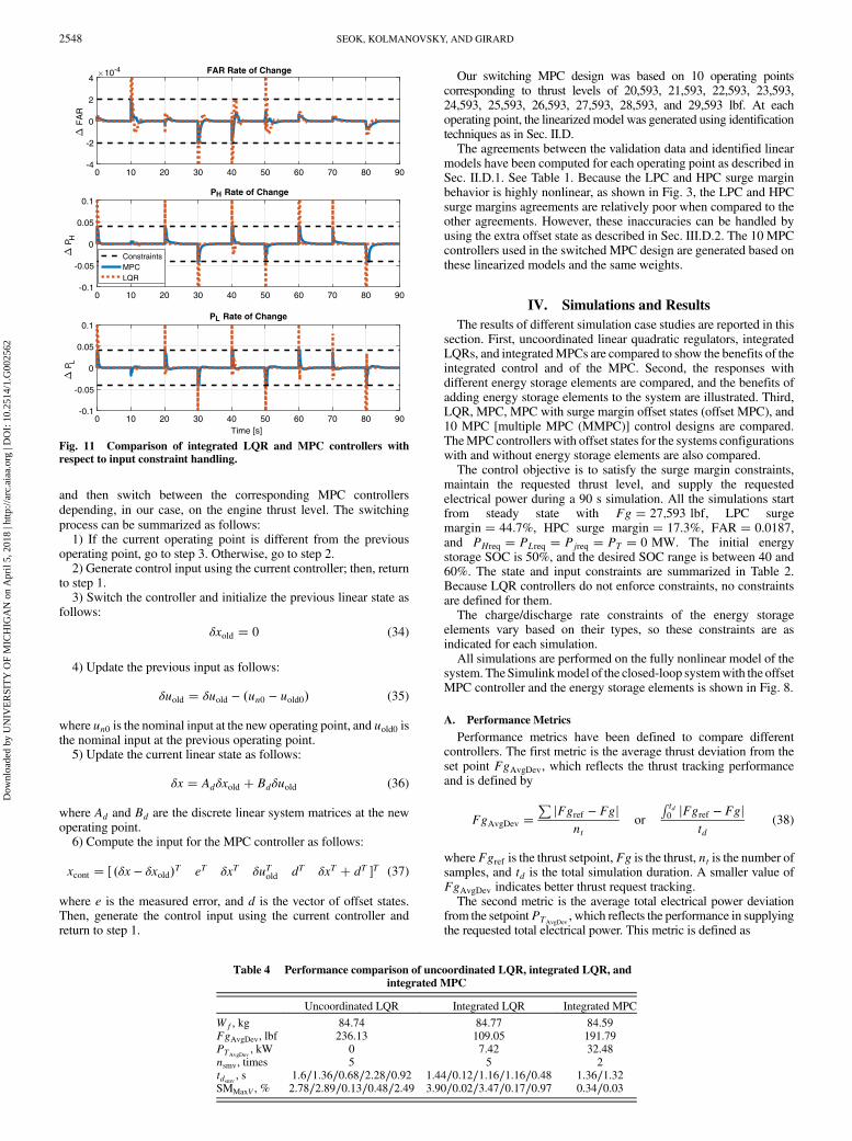
Our switching MPC design was based on 10 operating pointscorresponding to thrust levels of 20,593, 21,593, 22,593, 23,593,24,593, 25,593, 26,593, 27,593, 28,593, and 29,593 lbf. At eachoperating point, the linearized model was generated using identificationtechniques as in Sec. II.D.The agreements between the validation data and identified linear
models have been computed for each operating point as described inSec. II.D.1. See Table 1. Because the LPC and HPC surge marginbehavior is highly nonlinear, as shown in Fig. 3, the LPC and HPCsurge margins agreements are relatively poor when compared to theother agreements. However, these inaccuracies can be handled byusing the extra offset state as described in Sec. III.D.2. The 10 MPCcontrollers used in the switched MPC design are generated based onthese linearized models and the same weights.
IV. Simulations and Results
The results of different simulation case studies are reported in thissection. First, uncoordinated linear quadratic regulators, integratedLQRs, and integratedMPCs are compared to show the benefits of theintegrated control and of the MPC. Second, the responses withdifferent energy storage elements are compared, and the benefits ofadding energy storage elements to the system are illustrated. Third,LQR, MPC, MPC with surge margin offset states (offset MPC), and10 MPC [multiple MPC (MMPC)] control designs are compared.TheMPC controllers with offset states for the systems configurationswith and without energy storage elements are also compared.The control objective is to satisfy the surge margin constraints,
maintain the requested thrust level, and supply the requestedelectrical power during a 90 s simulation. All the simulations startfrom steady state with Fg � 27;593 lbf, LPC surgemargin � 44.7%, HPC surge margin � 17.3%, FAR � 0.0187,and PHreq � PLreq � Pjreq � PT � 0 MW. The initial energystorage SOC is 50%, and the desired SOC range is between 40 and60%. The state and input constraints are summarized in Table 2.Because LQR controllers do not enforce constraints, no constraintsare defined for them.The charge/discharge rate constraints of the energy storage
elements vary based on their types, so these constraints are asindicated for each simulation.All simulations are performed on the fully nonlinear model of the
system. The Simulinkmodel of the closed-loop systemwith the offsetMPC controller and the energy storage elements is shown in Fig. 8.
A. Performance Metrics
Performance metrics have been defined to compare differentcontrollers. The first metric is the average thrust deviation from theset point FgAvgDev, which reflects the thrust tracking performanceand is defined by
FgAvgDev �P jFgref − Fgj
ntor
R td0 jFgref − Fgj
td(38)
whereFgref is the thrust setpoint,Fg is the thrust, nt is the number ofsamples, and td is the total simulation duration. A smaller value ofFgAvgDev indicates better thrust request tracking.The second metric is the average total electrical power deviation
from the setpointPTAvgDev, which reflects the performance in supplying
the requested total electrical power. This metric is defined as
0 10 20 30 40 50 60 70 80 90-4
-2
0
2
4 F
AR
10-4 FAR Rate of Change
0 10 20 30 40 50 60 70 80 90-0.1
-0.05
0
0.05
0.1
PH
PH Rate of Change
0 10 20 30 40 50 60 70 80 90Time [s]
-0.1
-0.05
0
0.05
0.1
PL
PL Rate of Change
ConstraintsMPCLQR
Fig. 11 Comparison of integrated LQR and MPC controllers withrespect to input constraint handling.
, s 1.36∕1.32 1.32 1.36∕1.72 1.32∕0.76SMMaxV 0.34∕0.03 0.34 0.34∕0.06 0.34∕0.01
2.4
2.6
2.8
3
3.2
Fg
[lbf]
Thrust
0
1
2
P T [M
W]
Total Electrical Power
ReferenceConstraintBatteryCapacitor
0 10 20 30 40 50 60 70 80 90
0 10 20 30 40 50 60 70 80 90
0 10 20 30 40 50 60 70 80 90
Time [s]
20
40
60
80
SO
C [%
]
SOC
60 62 64 66 68 70 72 74 762.73
2.74
2.75
2.76
2.77
Fg
[lbf]
× 104×104 Thrust
18 20 22 24 26 28 30 32Time [s]
-0.5
0
0.5
1
1.5
2
2.5
P T [M
W]
Total Electrical Power
ReferenceConstraintBatteryCapacitor
Fig. 13 Comparison of battery and ultracapacitor packs.
2550 SEOK, KOLMANOVSKY, AND GIRARD
Dow
nloa
ded
by U
NIV
ER
SIT
Y O
F M
ICH
IGA
N o
n A
pril
5, 2
018
| http
://ar
c.ai
aa.o
rg |
DO
I: 1
0.25
14/1
.G00
2562
on aircraft. Note that, currently, relatively small stored energy isconsidered compared to our electrical load requests. The specificationsof the energy storage elements are shown in Table 6.There are clearly differences between the battery pack and the
ultracapacitor pack in terms of the stored energy and the discharge rate.The battery pack hasmuch larger stored energy than the ultracapacitorpack, but the ultracapacitor pack has a much faster discharge rate thanthe battery pack. The battery–ultracapacitor packs can take advantageof both characteristics. Based on the specifications in Table 6, thecontroller parameters and the energy storage element input constraints(charge/discharge rate constraints) are defined as shown in Table 7.All of the MPC controllers designed for systems with three
different storage element configurations use the same controllerparameters and constraints, except for the constraints on Pj that aredetermined based on the discharge rate of the energy storageelements. Constraints on _Pj are not considered. The simulationresults of MPC with the battery pack and the ultracapacitor pack areshown in Fig. 13.There are clear differences in the responses observed for the
two types of energy storage elements. The SOC of the ultracapacitorpack varies more than the SOC of the battery pack because theultracapacitor pack has much smaller stored energy than the batterypack, whereas the ultracapacitor pack is much faster than the batterypack, so it can supply the electrical loads very quickly; see the right-bottom subfigure, which shows the time history of the total electricalpower in the time interval between 18 and 32 s. However, due tolimited stored energy, the ultracapacitor cannot supply the electricalloads for a long time; instead, it needs to be recharged to recover aSOC in the 40–60% range, as shown in the left-bottom SOCsubfigure in the time interval between 20 and 25 s. Meanwhile, thebattery pack allows for better thrust command tracking, as shown inthe right-upper subfigure in Fig. 13,which represents the trajectory ofthrust in the time interval between 60 and 75 s. This is reasonable,given the large stored energy in the battery pack. The battery pack candeliver electrical power for a long time, which helps the gas turbineengine to use power for thrust generation instead of supplying thegenerators to satisfy the loads. In addition, the battery pack reducessurge margin violations, as shown in Table 8. Thus, for fasterelectrical loads supplying, the ultracapacitor pack appears to be asuitable energy storage choice; however, for faster thrust responsesand stable gas turbine engine operation, the battery pack is preferred.We next compare cases without and with the battery–
ultracapacitor pack that take advantage of the characteristics of
both types of energy storage elements. The simulation results are
shown in Fig. 14.
As shown in the right subfigures in Fig. 14, with the energy storage
element, the controller has better thrust and electrical power tracking.
The comparison of the performance of all the cases is shown in
Table 8. All energy storage element cases yield better performance
than the case without the energy storage element, except for the
second surge margin violation with the ultracapacitor pack. The
second surge margin violation for the ultracapacitor pack is longer
and larger than in the case without energy storage elements. This
violation likely occurs because the ultracapacitor pack needs to be
charged frequently, which requires the gas turbine engine to provide
more output than in the case without the ultracapacitor. Thus, using
the battery–ultracapacitor pack appears to be the preferred choice
from the perspective of system response to thrust commands and
electrical loads; and if the impact on weight, packaging, and cost is
not considered.
Note that the energy storage elements are beneficial, based on our
simulation results, despite the fact that their stored energy is limited in
this study. Evenmore substantial benefits are expected for the energy
storage elements with larger stored energy in future MEA.
Thrust
Total Electrical Power
ReferenceConstraintWithout Energy StorageWith Energy Storage
SOCConstraintsBatteryUltracapacitor
Thrust
Total Electrical Power
ReferenceConstraintWithout Energy StorageWith Energy Storage
18 20 22 24 26 28 30 32Time [s]
-0.5
0
0.5
1
1.5
2
2.5
P T [M
W]
60 62 64 66 68 70 72 74 762.73
2.74
2.75
2.76
2.77
Fg
[lbf]
× 104
2.4
2.6
2.8
3
3.2
Fg
[lbf]
0 40 50 60 70 80 90
0
1
2
P T [M
W]
0 10 20 30 40 50 60 70 80 90
0 10 20 30 40 50 60 70 80 90Time [s]
20
40
60
80
SO
C [%
]
Fig. 14 Comparison of controller performance without and with energy storage elements.
Table 9 Parameters for LQR, MPC, offset MPC, andMMPC controllers
D. Comparison of LQR, MPC, Offset MPC, and MMPC Controllers
In this section, the LQR, MPC, offset MPC, and MMPCcontrollers are compared. The MMPC controller based onlinearizations at multiple (10 in our case) operating points and theMPC controller with extra offset states are considered as potentialapproaches to better deal with the nonlinearities. For the purpose ofquantifying the potential benefits of these design steps, the energystorage elements are not included in the analysis, and a broader rangeof thrust profiles is used compared to the previous simulations. Thecontroller parameters are shown in Table 9.For all the controllers, the same parameters and constraints are
used. The closed-loop performance comparison is shown in Table 10.As expected, the LQR controller yields the best thrust and
electrical load tracking, but it violates the surge margin constraintsfour times with amaximum of 3.9%. It also consumes the largest fuelamount. The MPC controller is able to reduce the surge marginviolations; nevertheless, it violates the surge margin constraint onceat 5.36 s with a maximum violation of 1.06%. This violation is likelydue to the discrepancy between the prediction model and the actualnonlinear plant behavior. The MMPC design yields better thrust andelectrical loads tracking than the MPC controller, but the surgemargin constraint violation is longer and has larger magnitude thanthe MPC controller, which is likely due to surge margin predictionbeing insufficiently accurate. The offset MPC design yields verysimilar tracking performance to that of theMPC controller, and it hasno violation of the surge margin constraint. The simulation results ofthe MPC, MMPC, and offset MPC controllers are shown in Fig. 15.The black vertical lines indicate the switching time instants for
MMPC controllers. As observed, switching does not cause improperbehaviors of the system. For most of the simulation, all threecontrollers yield similar results, but the major differences can befound in the time interval between 60 and 80 s. Specifically, between60 and 70 s, the MPC controller assumes that it does not have anavailable HPC surge margin because of inaccurate surge marginestimation due to being far from the operating point. Thus, it does nottrack the thrust setpoint aggressively, whereas the MMPC and offsetMPC controllers are able to correctly account for the available HPCsurge margin; hence, they track the thrust setpoint faster than theMPC controller. In the time interval between 70 and 80 s, the MPCand MMPC controllers incorrectly assess that there is an availableHPC surgemargin, so they track the thrust setpoint aggressively; but,the offset MPC assesses that there is no available surge margin, so ittracks the thrust setpoint slowly to satisfy the HPC surge margin
constraint and uses the available LPC surge margin. Thus, the offset
MPC performs best in this simulation.To confirm that the offset MPC is a good design choice, an energy
storage element (the battery–ultracapacitor pack) is added to the offset
MPC controller, and the cases without and with the energy storage
element are compared to each other. The controller parameters and the
constraints can be found in Tables 2, 7, and 9. The performance
comparison is shown in Table 11.As shown in Table 11, both the thrust and the total electrical power
tracking performance are improved with the addition of the energy
storage, especially in terms of the total electrical power tracking
performance. The fuel consumption is increased as a penalty for
better tracking performance, but the increased amount is relatively
small. The surge margin constraints are perfectly satisfied for both
controllers. The simulation results of offsetMPC controllers with and
without energy storage elements are shown in Fig. 16.As the left subfigures in Fig. 16 show, the offset MPC with energy
storage elements shows better thrust and total electrical power
tracking. Both SOCs, especially for the ultracapacitor pack, violate
the SOC constraint a small number of times to deal with transient
thrust and electrical power changes, but they quickly recover to their
constrained levels. As shown in the right subfigures, for both
controllers, the power difference between the two generators stays
within the optimal power split ranges for most of the time, which
corresponds to safe and efficient operation.
E. Simulation Results for Offset MPC with and Without Sensor Noise
In this section, sensor noise is added to the measurements to verify
the robustness of the offset MPC controller, and the responses with
and without sensor noise are compared. Specifically, a zero mean
2
2.2
2.4
2.6
2.8
3
3.2
Fg
[lbf]
Thrust
-0.5
0
0.5
1
1.5
2
2.5
P T [M
W]
Total Electrical Power
ReferenceConstraintSingle MPC10 MPCsSingle MPC with offset
20
25
30
35
40
45
50
Sur
ge M
argi
n [%
]
LPC Surge Margin
12
14
16
18
20
22
Sur
ge M
argi
n [%
]
HPC Surge Margin
ConstraintSingle MPC10 MPCsSingle MPC with offset
0 10 20 30 40 50 60 70 80 90Time [s]
0 10 20 30 40 50 60 70 80 90Time [s]
0 10 20 30 40 50 60 70 80 90Time [s]
0 10 20 30 40 50 60 70 80 90
104
Fig. 15 Comparison of single MPC, MMPC, and single MPC with offset state controllers.
Table 11 Performance comparison of offsetMPCwith and without energy storage elements
Offset MPC
Without With BAT–UCAP pack
Wf , kg 74.28 74.41FgAvgDev, lbf 718.93 672.91PTAvgDev
, kW 101.14 71.35nsmv, times 0 0tdsmv
, s 0 0SMMaxV , % 0 0
2552 SEOK, KOLMANOVSKY, AND GIRARD
Dow
nloa
ded
by U
NIV
ER
SIT
Y O
F M
ICH
IGA
N o
n A
pril
5, 2
018
| http
://ar
c.ai
aa.o
rg |
DO
I: 1
0.25
14/1
.G00
2562
standard deviation Gaussian noise of 0.1% is added to the thrust, aswell as the LPC and HPC surge margins measurements. Thesimulation results of offsetMPCwith andwithout sensor noise for thesystem configuration with the battery–ultracapacitor are shownin Fig. 17.The simulation results show that the offset MPC controller is able
to handle the sensor noise. In the time interval between 70 to 80 s,
when high electrical power is required and the thrust increment is
requested near the HPC surge margin limit, some oscillations are
observed because of the sensor noise, but the controller is able to
handle the situation without having surge margin violations. Note
that the computational delay can be accommodated by using the
advanced-step MPC [40]; other delays, if they exist, can be handled
by augmenting the discrete-time model with extra delay states.
V. Conclusions
In this paper, the development of a coordinated control strategy fora gas turbine engine, an advanced dual-generator subsystem, andenergy storage elements for more-electrical aircraft and all-electricalaircraft in the presence of large transient thrust and electrical loadshas been pursued. The control design exploited rate-based modelpredictive control, for which various enhancements and designoptions have been considered and analyzed. Specifically, singleMPC, multiple MPC, and offset MPC strategies were applied andcompared to uncoordinated linear quadratic regulator and integratedLQR strategies in full nonlinear model simulations.The comparison of closed-loop responses for the cases of the
uncoordinated LQR and integrated LQR indicated that the integratedcontrol was capable of outperforming uncoordinated control in terms
2
2.5
3
3.5
Fg
[lbf]
× 104 Thrust
0
1
2
P T [M
W]
Total Electrical Power
ReferenceConstraintWithout Energy StorageWith Energy Storage
0
20
40
60
80
SO
C [%
]
SOCConstraintsBatteryUltracapacitor
-0.5
0
0.5
1
1.5Electrical Power Difference between HPC & LPC Gens
Fig. 16 Comparison of offset MPC with and without energy storage elements.
2
2.2
2.4
2.6
2.8
3
3.2
Fg
[lbf]
104 Thrust
-0.5
0
0.5
1
1.5
2
2.5
P T [M
W]
Total Electrical Power
ReferenceConstraintWith NoiseWithout Noise
20
25
30
35
40
45
50
Sur
ge M
argi
n [%
]
LPC Surge Margin
12
14
16
18
20
22
Sur
ge M
argi
n [%
]
HPC Surge Margin
ConstraintWith NoiseWithout Noise
0 10 20 30 40 50 60 70 80 90Time [s]
0 10 20 30 40 50 60 70 80 90Time [s]
0 10 20 30 40 50 60 70 80 90Time [s]
0 10 20 30 40 50 60 70 80 90
Fig. 17 Comparison of offset MPC controllers with and without sensor noise.
SEOK, KOLMANOVSKY, AND GIRARD 2553
Dow
nloa
ded
by U
NIV
ER
SIT
Y O
F M
ICH
IGA
N o
n A
pril
5, 2
018
| http
://ar
c.ai
aa.o
rg |
DO
I: 1
0.25
14/1
.G00
2562
of tracking performance. The integrated LQR controller yieldedbetter thrust and total electrical power tracking than the integratedMPC controller: however, with more surge margin constraintviolations and without granting any protection against violation ofother constraints.To improve prediction model accuracy, MMPC and offset MPC
design approaches were pursued. In the latter case, auxiliary offsetstateswere used to represent the error between the linearmodel-basedestimates of the constrained outputs and their actual value from thenonlinear model. The simulation results showed that a single MPCwith offset states was able to satisfy the surge margin constraints,whereas MMPC, which is a more complex controller, had someconstraint violations. Thus, the single rate-based offset MPCcontroller appeared to be the best strategy to control the system. Theclosed-loop system performance with different types of energystorage elements was also analyzed, with the combined battery andthe ultracapacitor pack providing the best solution; however, theweight and size impact of such an approach need to be carefullyanalyzed. Including energy storage elements into the systemimproved performance. For instance, in the current simulations, theoffset MPC controller with the battery–ultracapacitor pack improvedthe average thrust deviation by 6.4%, the settling time of thrust by3.47%, the average total electrical power tracking by 29.45%, and thesettling time of the total electrical power by 8.65% as compared to anoffset MPC controller applied to the system without energy storageand without any constraint violations. In addition, the offset MPCcontroller was able to handle sensor noise. The current results supportthe perspective that the aircraft architecture with dual generatorsattached to different gas turbine engine shafts and a battery–ultracapacitor pack, controlled by a single offset MPC controller, isappealing in terms of fast, safe, and efficient thrust and electrical loaddelivery for future MEA and AEA.
Acknowledgments
Theworkwas funded in part byTheBoeingCompany. The authorswould like to thank Brandon Hencey from the U.S. Air ForceResearch Laboratory for technical discussions and comments.
References
[1] Moir, I., and Seabridge, A., Aircraft Systems: Mechanical, Electrical
and Avionics Subsystems Integration, 3rd ed., Wiley, New York, 2008,Chaps. 1, 5, 10.
[2] Rosero, J. A., Ortega, J. A., Aldabas, E., and Romeral, L., “MovingTowards a More Electric Aircraft,” IEEE Aerospace and Electronic
Systems Magazine, Vol. 22, No. 3, March 2007, pp. 3–9.doi:10.1109/MAES.2007.340500
[3] Luongo, C. A., Masson, P. J., Nam, T., Mavris, D., Kim, H. D.,Brown, G. V., Waters, M., and Hall, D., “Next Generation More-Electric Aircraft: A Potential Application for HTS Superconductors,”IEEE Transactions on Applied Superconductivity, Vol. 19, No. 3,June 2009, pp. 1055–1068.doi:10.1109/TASC.2009.2019021
[4] Felder, J., Kim, H., and Brown, G., “Turboelectric DistributedPropulsion Engine Cycle Analysis for Hybrid-Wing-Body Aircraft,”AIAA Aerospace Sciences Meeting Including the New Horizons Forum
and Aerospace Exposition, AIAA Paper 2009-1132, Jan. 2009.doi:10.2514/6.2009-1132
[5] Kim, H. D., “Distributed Propulsion Vehicles,” 27th International
Congress of the Aeronautical Sciences, ICAS, Bonn, Germany,Sept. 2010.
[6] McNab, I. R., “Pulsed Power for Electric Guns,” IEEE Transactions on
Magnetics, Vol. 33, No. 1, Jan. 1997, pp. 453–460.doi:10.1109/20.560055
[7] “Technology Horizons: AVision for Air Force Science and Technology2010-30,” U.S. Air Force TR AF/ST-TR-10-01-PR, 2010.
[8] Behbahani, A., et al., “Status, Vision, and Challenges of an IntelligentDistributed Engine Control Architecture,” Soc. of AutomotiveEngineers TP 2007-01-3859, Warrendale, PA, 2007.doi:10.4271/2007-01-3859
[9] Behbahani, A. R., Von Moll, A., Zeller, R., and Ordo, J., “AircraftIntegration Challenges and Opportunities for Distributed IntelligentControl, Power, Thermal Management, Diagnostic and Prognostic
Systems,” Soc. of Automotive Engineers TP 2014-01-2161, Warrendale,PA, 2014.doi:10.4271/2014-01-2161
[10] Litt, J. S., Simon, D. L., Garg, S., Guo, T.-H., Mercer, C., Millar, R.,Behbahani, A., Bajwa, A., and Jensen, D. T., “A Survey of Intelligent
Control and Health Management Technologies for Aircraft Propulsion
Systems,” Journal of Aerospace Computing, Information, and
Communication, Vol. 1, No. 12, 2004, pp. 543–563.
doi:10.2514/1.13048[11] DeSimio, M. P., Hencey, B. M., and Parry, A. C., “Online Prognostics
for Fuel Thermal Management System,” ASME 2015 Dynamic Systems
and Control Conference, American Soc. of Mechanical Engineers
Paper V001T08A003, Fairfield, NJ, Oct. 2015.
doi:10.1115/DSCC2015-9842[12] Richter, H., Advanced Control of Turbofan Engines, 1st ed., Springer,
New York, 2012, Chap. 9.[13] DeCastro, J. A., “Rate-Based Model Predictive Control of Turbofan
Engine Clearance,” Journal of Propulsion and Power, Vol. 23, No. 4,2007, pp. 804–813.doi:10.2514/1.25846
[14] Fuller, J., Das, I., Potra, F., and Ji, J., “System and Method ofApplying Interior Point Method for Online Model Predictive Control
of Gas Turbine Engines,” U.S. Patent Application 11/150,703,
June 2005.[15] Huang, M., Zaseck, K., Butts, K., and Kolmanovsky, I., “Rate-Based
Model Predictive Controller for Diesel Engine Air Path: Design andExperimental Evaluation,” IEEE Transactions on Control Systems
Technology, Vol. 24, No. 6, March 2016, pp. 1922–1935.doi:10.1109/TCST.2016.2529503
[16] Herceg, M., Kvasnica, M., Jones, C. N., and Morari, M., “Multi-Parametric Toolbox (MPT) 3.0,” European Control Conference, IEEEPubl., Piscataway,NJ, July 2013, pp. 502–510, http://control.ee.ethz.ch/~mpt.
[17] Mitcham, A. J., and Cullen, J. J. A., “Permanent Magnet GeneratorOptions for the More Electric Aircraft,” International Conference on
Power Electronics, Machines and Drives, IET, Stevenage, U.K.,
June 2002, pp. 241–254.
doi:10.1049/cp:20020121[18] Rakhra, P., Norman, P. J., Galloway, S. J., and Burt, G. M., “Modelling
and Simulation of a MEA Twin Generator UAV Electrical PowerSystem,” International Proceedings of Universities’ Power EngineeringConference, VDE, Berlin, Germany, Sept. 2011, pp. 1–5.
[19] Muehlbauer,K., andGerling,D., “Two-Generator-Concepts for ElectricPower Generation in More Electric Aircraft Engine,” International
Conference on Electrical Machines, IEEE Publ., Piscataway, NJ,
Sept. 2010, pp. 1–5.
doi:10.1109/ICELMACH.2010.5607966[20] Alnajjar, M., and Gerling, D., “Control of Three-Source High Voltage
Power Network for More Electric Aircraft,” International Symposiumon Power Electronics, Electrical Drives, Automation andMotion, IEEEPubl., Piscataway, NJ, June 2014, pp. 232–237.doi:10.1109/SPEEDAM.2014.6871906
[21] Kim, J. S., Powell, K. M., and Edgar, T. F., “Nonlinear ModelPredictive Control for a Heavy-Duty Gas Turbine Power Plant,”AmericanControl Conference, IEEEPubl., Piscataway,NJ, June2013,pp. 2952–2957.doi:10.1109/ACC.2013.6580283
[22] Thirunavukarasu, E., Fang, R., Khan, J. A., andDougal, R., “Evaluationof Gas Turbine Engine Dynamic Interaction with Electrical andThermal System,” Electric Ship Technologies Symposium, IEEE Publ.,Piscataway, NJ, April 2013, pp. 442–448.doi:10.1109/ESTS.2013.6523773
[23] Norman, P. J., Galloway, S. J., Burt, G. M., Hill, J. E., and Trainer, D.R., “Evaluation of the Dynamic Interactions Between Aircraft GasTurbine Engine and Electrical System,” IET Conference on Power
Electronics, Machines and Drives, IET, Stevenage, U.K., April 2008,pp. 671–675.doi:10.1049/cp:20080606
[24] Todd,R.,Wu,D., dos SantosGirio, J. A., Poucand,M., andForsyth, A. J.,“Supercapacitor-Based Energy Management for Future AircraftSystems,” Applied Power Electronics Conference and Exposition, IEEEPubl., Piscataway, NJ, Feb. 2010, pp. 1306–1312.doi:10.1109/APEC.2010.5433398
[25] Shahsavari, B., Maasoumy, M., Sangiovanni-Vincentelli, A., andHorowitz, R., “Stochastic Model Predictive Control Design for LoadManagement System of Aircraft Electrical Power Distribution,”American Control Conference, IEEE Publ., Piscataway, NJ, July 2015,pp. 3649–3655.doi:10.1109/ACC.2015.7171897
[26] Jaw, L. C., and Mattingly, J., Aircraft Engine Controls: Design, SystemAnalysis, and Health Monitoring, 1st ed., AIAA, Reston, VA, 2010,Chaps. 2–7.
[27] Chapman, J. W., Lavelle, T. M., Litt, J. S., May, R. D., and Guo, T.-H.,“PropulsionSystemSimulationUsing theToolbox for theModeling andAnalysis of Thermodynamic Systems (T-MATS),” Propulsion and
Energy Forum, AIAA Paper 2014-3929, July 2014.doi:10.2514/6.2014-3929
[28] Zinnecker,A.,Chapman, J.W.,Lavelle,T.M., andLitt, J. S.,“Developmentof a Twin-Spool Turbofan Engine Simulation Using the Toolbox forModeling and Analysis of Thermodynamic Systems (T-MATS),”Propulsion and Energy Forum, AIAA Paper 2014-3930, July 2014.doi:10.2514/6.2014-3930
[29] Chapman, J.W., Lavelle, T.M., Litt, J. S., andGuo, T.-H., “AProcess forthe Creation of T-MATS Propulsion SystemModels from NPSS Data,”Propulsion and Energy Forum, AIAA Paper 2014-3931, July 2014.doi:10.2514/6.2014-3931
[30] Seok, J., Kolmanovsky, I., and Girard, A., “Integrated/CoordinatedControl of Aircraft Gas Turbine Engine and Electrical Power System:Towards Large Electrical LoadHandling,” IEEEConference onDecision
and Control, IEEE Publ., Piscataway, NJ, Dec. 2016, pp. 3183–3189.doi:10.1109/CDC.2016.7798747
[31] Corbett,M., Lamm,P.,McNichols, J., Boyd,M., andWolff,M., “Effectsof Transient Power Extraction on an Integrated Hardware-in-the-LoopAircraft/Propulsion/Power System,” Soc. of Automotive Engineers TP2008-01-2926, Warrendale, PA, 2008.doi:10.4271/2008-01-2926
[32] Vahidi, A., Kolmanovsky, I., and Stefanopoulou, A., “ConstraintHandling in a Fuel Cell System: A Fast ReferenceGovernorApproach,”IEEE Transactions on Control Systems Technology, Vol. 15, No. 1,2007, pp. 86–98.doi:10.1109/TCST.2006.883242
[33] Garone, E., Di Cairano, S., and Kolmanovsky, I., “Reference andCommand Governors for Systems with Constraints: A Survey of
Their Theory and Application,” Automatica, Vol. 75, No. 1, 2017,pp. 306–328.doi:10.1016/j.automatica.2016.08.013
[34] DeLaat, J. C., Southwick, R. D., and Gallops, G. W., “High StabilityEngine Control (HISTEC),” 32nd Joint Propulsion Conference
Cosponsored by AIAA, ASME and SAE, AIAA Paper 1996-2586,July 1996.doi:10.2514/6.1996-2586
[35] Ortner, P., and del Re, L., “Predictive Control of a Diesel Engine AirPath,” IEEE Transactions on Control Systems Technology, Vol. 15,No. 3, 2007, pp. 449–456.doi:10.1109/TCST.2007.894638
[36] Di Cairano, S., and Tseng, H., “Driver-Assist Steering by Active FrontSteering and Differential Braking: Design, Implementation andExperimental Evaluation of a Switched Model Predictive ControlApproach,” IEEE Conference on Decision and Control, IEEE Publ.,Piscataway, NJ, Dec. 2010, pp. 2886–2891.doi:10.1109/CDC.2010.5716954
[37] Huang,M., Nakada, H., Polavarapu, S., Choroszucha, R., Butts, K., andKolmanovsky, I., “Towards Combining Nonlinear and PredictiveControl of Diesel Engines,” American Control Conference, IEEE Publ.,Piscataway, NJ, June 2013, pp. 2846–2853.doi:10.1109/ACC.2013.6580266
[38] “Nanophosphate Lithium Ion Prismatic Pouch Cell AMP20M1HD-A,”http://liionbms.com/pdf/a123/AMP20M1HD-A.pdf [retrieved20 April 2017].
[39] “Datasheet: K2Ultracapacutors–2.85V/3400F,”Maxwell TechnologiesDocument 3000619-EN.3, San Diego, CA, http://www.maxwell.com/images/documents/K2_2_85V_DS_3000619EN_3_.pdf [retrieved20 April 2017].
[40] Zavala, V. M., and Biegler, L. T., “The Advanced-Step NMPCController: Optimality, Stability and Robustness,” Automatica, Vol. 45,No. 1, 2009, pp. 86–93.doi:10.1016/j.automatica.2008.06.011