University of Bath | LUMINAR EMRP Project | July 2016

Coping with Thermal Expansion in Large Volume Metrology

Good Practice Guide

2

Contents 1 Guide Information ........................................................................................... 4

2 Introduction ..................................................................................................... 5

3 Hybrid Metrology ............................................................................................. 6

4 Temperature Measurement Strategy .............................................................. 9

4.1 Temperature Measurement Planning .................................................... 10

5 Displacement Prediction Simulation .............................................................. 13

5.1 Geometric Considerations ..................................................................... 15

5.2 Meshing ................................................................................................. 16

5.3 Thermal Analysis ................................................................................... 16

5.4 Structural Analysis ................................................................................. 17

5.5 Solution and results ............................................................................... 17

6 Thermal Compensation ................................................................................. 18

6.1 Coordinate Correction ............................................................................ 18

6.2 Distance Correction ............................................................................... 19

7 Model Validation ........................................................................................... 19

8 Uncertainty Evaluation .................................................................................. 21

9 Acknowledgements ....................................................................................... 22

10 Bibliography and Further Reading............................................................. 22

3

Figures

Figure 1 - Illustration of one possible configuration of Hybrid Metrology System

for thermal compensation [6] ................................................................ 7

Figure 2 - Table showing the required change in temperature detectable to be

able to resolve thermal expansion from 10-50 microns over different

lengths in different materials [8] ........................................................... 9

Figure 3 - Diagram showing the general steps of building and executing a

comprehensive temperature measurement plan ................................ 11

Figure 4 - Taxonomy of seven temperature measurement technologies of

particular interest in the application of thermal compensation in

assembly environments [8, 10] .......................................................... 12

Figure 5 - General steps of finite element analysis from temperature data to

displacement predictions for thermal compensation .......................... 14

4

1 Guide Information

What is it about?

This guide is about coping with thermal expansion (or contraction) in large volume

metrology environments that are not closely controlled.

Who is it for?

This guide is for users who wish to measure dimensions in a range of environments

with a clearer idea of the thermal impact. The methodology can also be extended

to those in manufacturing situations who wish to predict the impact of thermal

expansion upon assembly operations.

What is its purpose?

The purpose is to outline a methodology for mitigating the effect of thermal

expansion in large volume metrology.

What is the prerequisite knowledge?

The guide covers topics from entry to advanced levels. It assumes the reader has

some scientific knowledge, and some familiarity with large volume metrology.

5

2 Introduction

Measurement of length dimensions is of great importance to a great many

applications from scientific studies to manufacturing. In order to produce

measurement results that we can rely upon, there is a need to understand the

environment in which the measurements are taken as these will have a physical

effect upon the object that is being measured.

In many cases, the largest source of measurement uncertainty is thermal

expansion and as a result, a standard measurement temperature has been set at

20 ºC [1]. Where possible, action is taken to ensure that in places where

measurements are being taken the temperature is closely controlled. A coordinate

measuring machine (CMM) in a laboratory is often held close to this temperature

using continuous monitoring that can provide closed-loop feedback to the heating

system. Objects to be measured are allowed to ‘soak’ in this environment until

they match the desired ambient temperature of the room. Whilst there is some

degree of instability around this temperature, this is closely characterized and

therefore managed appropriately.

However, what happens when we are forced to carry out measurements in an

environment that is not temperature controlled – or even loosely controlled? One

“obvious” answer is to measure the ambient temperature, and scale all of the

measurements according to the material’s coefficient of thermal expansion (CTE).

In cases where we have a choice of material and all other requirements are

satisfied, the material that exhibits a thermal expansion that is relatively low can

be selected. This can be effective in some situations for reducing thermal impact

but such materials can be more expensive.

There are many situations in which closely controlling the temperature of the

environment simply cannot be achieved practically, or cost-effectively. For large

volume metrology, where measurements are carried out from several metres up

to several tens of metres, thermal issues become quite challenging [2, 3].

In a small volume, measurement of the ambient temperature around the part

results in a relatively small variation in temperature. The instinctive approach of

measuring the ambient temperature and uniformly scaling all of the dimensions

using the material’s CTE works well here. Larger volumes offer far more complex

ambient temperature distributions. Thermal gradients vertically in a volume for an

aerospace assembly environment for instance may be in excess of 5 ºC.

Depending upon the architecture, horizontal gradients can be similarly observed.

Further compounding this effect, the gradients are not necessarily linear, with

much steeper vertical gradients being formed very close to the floor and close to

6

the ceiling, for instance. Depending also upon the environment, there may be a

heat source causing a highly localized temperature distribution – a hot or cold spot.

Temperature by its nature is rarely static unless controlled. Even with the best

intentions, static temperature is an approximation. Over a short period of time (of

the order of seconds or minutes) the ambient temperature probably does not

change a great deal, but it may change over longer time intervals. So any method

of scaling has to be continually adapted with up-to-date temperature data from

around the volume.

Thermal effects are not the only effects at play. One other effect of particular

concern in large volume metrology is that of deflection under loading. This loading

could be due to the object’s own weight or the weight of another part being

supported during an assembly operation, for instance.

With these effects in mind and their impact on our understanding of the object that

is being measured, this guide aims to outline a method by which we can begin to

compensate for these effects. Recent research attention has been given to what

is known as a Hybrid Metrology approach. Generally speaking, the approach as

offered here is to continually monitor temperature around the measurement

volume. Using these measured temperature in computational simulation it is

possible to predict how the object is likely to be affected under these loads in terms

of point displacements. The resulting simulated displacements can then be added

to the measured coordinates to produce a measurement result that is closer to

what would be measured in an ideal metrology environment (if such an

environment were available).

Further information on dimensional measurement can be found in other Good

Practice Guides, which deal with dimensional metrology, specifically [4, 5].

3 Hybrid Metrology

‘Hybrid’ is a term that is used in a number of different fields, with a variety of

accompanying definitions. To clarify, the term hybrid metrology is used here to

describe an approach to measurement that combines the measurement of different

physical quantities with computational methods to produce final measurement

results. Following this definition, there are a number of ways in which such an

approach can be applied so the hybrid metrology framework has been designed

to be modular to allow for application-specific adaptation.

7

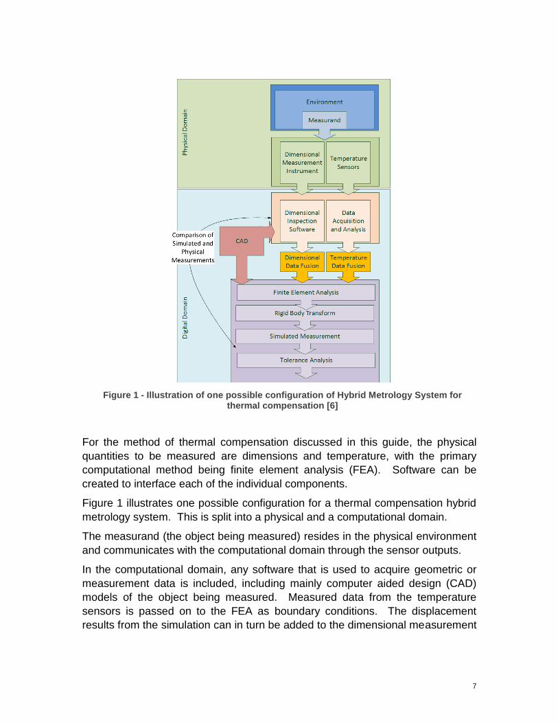
Figure 1 - Illustration of one possible configuration of Hybrid Metrology System for thermal compensation [6]

For the method of thermal compensation discussed in this guide, the physical

quantities to be measured are dimensions and temperature, with the primary

computational method being finite element analysis (FEA). Software can be

created to interface each of the individual components.

Figure 1 illustrates one possible configuration for a thermal compensation hybrid

metrology system. This is split into a physical and a computational domain.

The measurand (the object being measured) resides in the physical environment

and communicates with the computational domain through the sensor outputs.

In the computational domain, any software that is used to acquire geometric or

measurement data is included, including mainly computer aided design (CAD)

models of the object being measured. Measured data from the temperature

sensors is passed on to the FEA as boundary conditions. The displacement

results from the simulation can in turn be added to the dimensional measurement

8

results to create a simulated measurement. This simulated measurement may

then be used to predict tolerance stack-up throughout an assembly.

Throughout the use of the hybrid metrology system, the simulated measurements

can be compared to measured dimensions in order to validate the simulation,

particularly in the initial setup of the system. Closer agreement of dimensional

measurements to the simulated measurements means that there can be greater

confidence in the simulated measurements that are produced. Ideally, it is the goal

to use the minimum amount of dimensional measurement whilst having continual

simulated measurements to provide up-to-date displacement data using only

volumetric temperature data. This allows for adjustments to be made to processes,

products, tooling or the environment itself to negate these effects.

9

4 Temperature Measurement Strategy

Managing thermal effects naturally requires an understanding of the temperature

of the object you are trying to measure. The lower the uncertainty of the measured

temperature, the more accurate predictions can be made in the simulation of

thermal expansion. Further information about quantifying the uncertainty of

thermometers can be found in Good Practice Guide 125 [7].

It is important to gain some perspective in the role of temperature measurement in

the prediction of thermal expansion. This is partly for reference, but in particular

so that we have an idea of the type of sensors that may be required. Materials

with a larger coefficient of thermal expansion (CTE) require more sensitive

measurement techniques, as their dimensions vary more in response to a change

in temperature. Whilst a lot of data about CTE can be found for most materials, it

should be noted that the value of CTE for a material can vary and the values given

have some level of uncertainty associated. Not only does the CTE vary with

materials, but also depending on the starting temperature of the material as can

be seen in Figure 2. As a result, many material databases will quote the reference

temperature for the corresponding CTE value.

Figure 2 - Table showing the required change in temperature detectable to be able to resolve thermal expansion from 10-50 microns over different lengths in different materials [8]

10

4.1 Temperature Measurement Planning

There are a great many ways to measure temperature [9] and some are better

than others depending upon the particular application. Planning for temperature

measurement is vital but it is best if the plan includes some way to adapt to suit

the particular application where thermal compensation is required. With this in

mind, it is often best to test a number of configurations experimentally to ensure

they produce results that are useful – useful in this context could be defined as

how well the thermal expansion predictions can be validated by measurement data.

A strategy for developing tailored, reproducible temperature plans specifically for

large volume metrology and thermal compensation is currently being created. This

covers a number of the steps illustrated in Figure 3.

11

Figure 3 - Diagram showing the general steps of building and executing a comprehensive temperature measurement plan

At the outset, the production of a temperature measurement plan requires

knowledge of the environment in which the instrumentation is expected to operate.

Questions that need to be asked at this stage include:

What is the temperature range?

Can we use contact or non-contact sensors?

Are there any magnetic fields which might increase uncertainty?

Are there any radiation sources?

Where can we place our data acquisition hardware?

Now that we have a clearer definition of the environment, we can start to narrow

down which sensors can be selected. Of course for many applications another

Environmental survey

• Environmental measurement

• Practical considerations

• Uncertainty source identification

Temperature measurement

plan

• Sensor selection

• Data acquisition

• Sensor positioning

Hardware deployment

Simulation and dimensional

measurement agreement

• Temperature measurement

• Finite element analysis

• Dimensional measurement

Continuous Improvement

12

important constraint is the cost of the instrumentation. Seven sensors and their

associated classifications have been identified that are of interest for large volume

assembly environments, as seen in Figure 4.

Figure 4 - Taxonomy of seven temperature measurement technologies of particular interest in the application of thermal compensation in assembly environments [8, 10]

Once a balance has been achieved between the requirements of the application

and the economic constraints, an initial plan can be drafted as to where to position

all of the instrumentation. Whilst doing this, it is important to take a range of

measurements around the working volume in order to get a feel for the kind of

temperature distribution that is present. In places where there are steep gradients,

for example, it is beneficial to increase the sensor density.

Following the agreement of an initial measurement plan, the temperature sensor

network can be constructed. At this stage, validation experiments need to be

designed and executed in order to ascertain whether or not this sensor network is

providing reliable results. Validation is further discussed in section 7 of this guide

but essentially, the agreement between displacements under different thermal

loads needs to become the performance metric for the temperature measurement

13

plan. The plan can subsequently be altered for optimization purposes, such as

moving sensors to different positions. This process should then be repeated as

part of a continuous improvement strategy.

5 Displacement Prediction Simulation

Computer aided engineering (CAE) has been in use for decades and has conferred

a great many advantages. One of these advantages is being able to simulate a

range of conditions outside of what can easily be tested in reality. Traditionally, a

lot of the techniques for simulation have been used in design and planning, but

increasingly computational techniques are delivering value during processes.

The simulation method used for the prediction of displacements due to thermal

expansion, as briefly mentioned earlier in the guide is known as finite element

analysis (FEA). The finite element method (FEM) is well-established in the design

phase of product development, in order to improve and provide verification that

designs will perform as required for the intended application.

Other methods for simulating thermal expansion and distortion under loading are

available but FEA is the focus for this guide. FEA is widely used for these types of

calculation in industry and academia but it should be noted that any computational

method that can accept temperatures as a load condition to calculate localized

displacements could be applied for such an application. A range of books are

available on the subject [11-16]. FEA is an entire field of its own and so it is not

covered here in any depth. This section outlines some general considerations that

are important for successful application of this technique.

FEM is all about breaking down large structures into smaller elements, where

equations modelling physical laws can be set up and solved automatically.

Elements are usually small volumes (such as cuboids) defined by their vertices

(nodes) and edges. A collection of these elements together is referred to as a mesh

that covers the full geometry of the object to be analysed.

A number of types of analysis can be performed using a range of commercially

available software packages. One of the well-known dedicated software packages

for FEA is ANSYS [17] and this is used in this guide for example purposes. Other

packages include Abaqus [18], and Nastran [19]. Some CAD systems such as

Solidworks [20] include some level of FEA to perform simulation. As with other

types of software, the various packages have their own strengths and weaknesses,

but an in-depth comparison is not covered in this guide.

Generally speaking, FEA consists of a number of steps [11], regardless of which

software package is being used. It is important to be aware of these steps as each

14

software package’s performance in each of these steps forms a basis for

comparison. Some FEA packages deal only with specific steps, meaning that

further software is required to complete the analysis. The four main elements of

an FEA package are:

1) Pre-processor

2) Mesher

3) Solver

4) Post-processor

Thermal compensation generally requires a thermal analysis and structural

analysis. Thermal analysis calculates a full temperature distribution based upon

relevant thermal loads – that is to say, given the temperatures at some of the nodes,

it can calculate what the temperature is at all of the non-specified nodes depending

upon the properties (e.g. conductivity) and boundary conditions (e.g. convection)

that are specified.

The structural analysis can accept temperature data as boundary conditions to

calculate structural results such as displacement or stress. Using thermal and

structural analyses in series in this way is known as one-way direct coupling.

Figure 5 - General steps of finite element analysis from temperature data to displacement predictions for thermal compensation

In some cases it is possible to replace thermal analysis with other methods to

interpolate the temperature distribution that is applied to the geometry. As thermal

analysis can be time-consuming, it may sometimes be quicker and easier to opt

for a more simple interpolation scheme. When thermal expansion is driven by

relatively slowly changing ambient temperature, where there are more gentle

thermal gradients, interpolation can provide a quicker means to run a structural

analysis. Time is an important factor in a range of applications, but particularly for

manufacturing.

Displacement

data

Structural

analysis

Thermal

analysis

Temperature

data

15

In order for an analysis to be performed, FEA typically requires the following

actions to be completed:

Geometry modelling – provision of a CAD model file from an external source,

or CAD model generated within the FEA package

Meshing – the geometry is divided into elements and node and element

numbers are assigned

Material definition – material properties are assigned to the geometry

Boundary condition definition – constraints and loads are imposed on the

geometry to match the physical condition as closely as possible

Solving – using the boundary conditions and material properties, solutions

are calculated at each of the elements on the mesh

Post-processing – results can be viewed and analysed depending upon

requirements

5.1 Geometric Considerations

CAD geometry for FEA should be tested to ensure that it works within the FEA

software package without any problems. In some cases, CAD geometry may need

to be repaired, simplified or entirely remodelled. The more complex the CAD

model is, the more difficult it is to mesh. A finer and more complex mesh increases

the node count which means that the simulation takes much longer. It may be the

case that if the model is too complex, and then features need to be removed. In

thermal and structural analyses, it is important to identify which features are likely

to have a significant impact in the end result. Removing chamfers and fillets, for

example, often does not make a big difference to the final displacements but

significantly improves simulation times. This can be tested with the model that you

are intending to use.

Spending a lot of time deleting small parts and features from a complex CAD model

can become quite a messy process. There are times when it is best to try to rebuild

an “FEA-friendly” CAD model for simulations from scratch. Building FEA-friendly

CAD is all about identifying the features that are most important, and discarding

those which are not adding significant value to the analysis. Assemblies can

similarly cause problems and for thermal expansion analyses, there may be

occasions when you can model an assembly as a single part without impacting the

final results too heavily. Preparing a number of these test cases can be useful

throughout the validation phase.

16

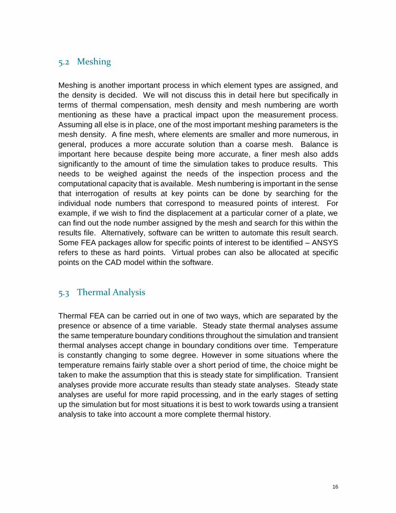
5.2 Meshing

Meshing is another important process in which element types are assigned, and

the density is decided. We will not discuss this in detail here but specifically in

terms of thermal compensation, mesh density and mesh numbering are worth

mentioning as these have a practical impact upon the measurement process.

Assuming all else is in place, one of the most important meshing parameters is the

mesh density. A fine mesh, where elements are smaller and more numerous, in

general, produces a more accurate solution than a coarse mesh. Balance is

important here because despite being more accurate, a finer mesh also adds

significantly to the amount of time the simulation takes to produce results. This

needs to be weighed against the needs of the inspection process and the

computational capacity that is available. Mesh numbering is important in the sense

that interrogation of results at key points can be done by searching for the

individual node numbers that correspond to measured points of interest. For

example, if we wish to find the displacement at a particular corner of a plate, we

can find out the node number assigned by the mesh and search for this within the

results file. Alternatively, software can be written to automate this result search.

Some FEA packages allow for specific points of interest to be identified – ANSYS

refers to these as hard points. Virtual probes can also be allocated at specific

points on the CAD model within the software.

5.3 Thermal Analysis

Thermal FEA can be carried out in one of two ways, which are separated by the

presence or absence of a time variable. Steady state thermal analyses assume

the same temperature boundary conditions throughout the simulation and transient

thermal analyses accept change in boundary conditions over time. Temperature

is constantly changing to some degree. However in some situations where the

temperature remains fairly stable over a short period of time, the choice might be

taken to make the assumption that this is steady state for simplification. Transient

analyses provide more accurate results than steady state analyses. Steady state

analyses are useful for more rapid processing, and in the early stages of setting

up the simulation but for most situations it is best to work towards using a transient

analysis to take into account a more complete thermal history.

17

5.4 Structural Analysis

Once the temperature distribution has been calculated for the entire geometry

under analysis, a structural analysis can be performed in order to determine

displacements. After thermal load assignment, other boundary conditions need to

be specified.

Before any loads are assigned, it is important to check the material properties are

correct and any uncertainty associated is noted. Stiffness and density significantly

impact displacement results so it is important to check these.

For the structural analysis, boundary conditions that we need to consider include:

Support conditions

Connections between parts

Support conditions need to be carefully considered and matched closely to the real

situation that is to be modelled. There is an option in most FEA packages to use

a fixed support. However, this must be used with care as it can in some instances

produce unusual and hinder overall movement of the structure - constraining

displacement is often more useful.

Connections between parts in an assembly are made more straightforward within

FEA packages but to make the selection that matches closely to the physical reality

can be challenging. Any information about connections can be useful. Are the

connections bonded or more elastic? Is there a frictional connection between two

parts? If there is some doubt as to how best to model connections, running the

simulations and comparing them to validation experiments is usually the best way

to approach the problem.

5.5 Solution and results

Solving the structural analysis reveals displacements for the geometry based upon

the input boundary conditions. Post-processing can be carried out easily in most

commercially available FEA packages and these often have a reporting function.

If preferred, results can be exported as a different file format, which can be useful

so that they can be integrated with the dimensional measurements. Commonly

used files are: text files (.txt), Excel files (.xls), and comma separated variable

(.csv) files.

18

6 Thermal Compensation

Once displacement data is taken from the simulation, simulated measurements

can be produced. Two methods for producing simulated measurements will be

given here. The first is for the correction of coordinate measurements and the

second is for length measurements between two points.

6.1 Coordinate Correction Coordinate measurement compensation is a very straightforward idea but the

direction in which an object is likely to expand can be a little more difficult to

predict in practice.

All that needs to be done is for measured coordinates to be added to their predicted

displacements resulting from the finite element analysis (FEA).

Coordinate Correction:

(𝑥’, 𝑦’, 𝑧’) = (𝑥 + 𝑑𝑥, 𝑦 + 𝑑𝑦, 𝑧 + 𝑑𝑧)

where:

(x’, y’, z’) are the simulated coordinates

(x, y, z) are the uncorrected coordinates

(dx, dy, dz) are the displacement predictions from simulation

This is mathematically straightforward, but the difficulty in the application of this

correction will often arise from two main areas.

The first of these challenges comes from the fact that this type of correction is

predicated upon the coordinate systems of the physical dimensional measurement

and the simulation being aligned. This can be most easily achieved by setting the

coordinate system appropriately within the simulation to match the dimensional

measurement. Alternatively, if for some reason the coordinate systems are not

exactly aligned, a rigid body transform can be used to match points from the

simulation to the dimensional measurement points.

The second problem can arise from the nature of the structure itself. Whilst the

magnitude of the predicted displacement may be in good agreement with initial

measurements, the direction in which the displacements are happening may be

slightly different, especially when the physical object is constrained in such a way

that a number of possibilities can arise. One way to manage this is to take a

19

number of test measurements and alter the geometry within the simulation to better

match the empirical data.

For example, a frame could be mounted upon the floor but the floor may not be

completely level. This can be observed through measurement as the frame has a

tendency to be displaced in one direction more significantly than another. Within

the simulation then, a rotation of the CAD model relative to gravity produces a

similar leaning effect. Alternatively, one might adapt the resulting geometry

mathematically in order to correct for such systematic errors.

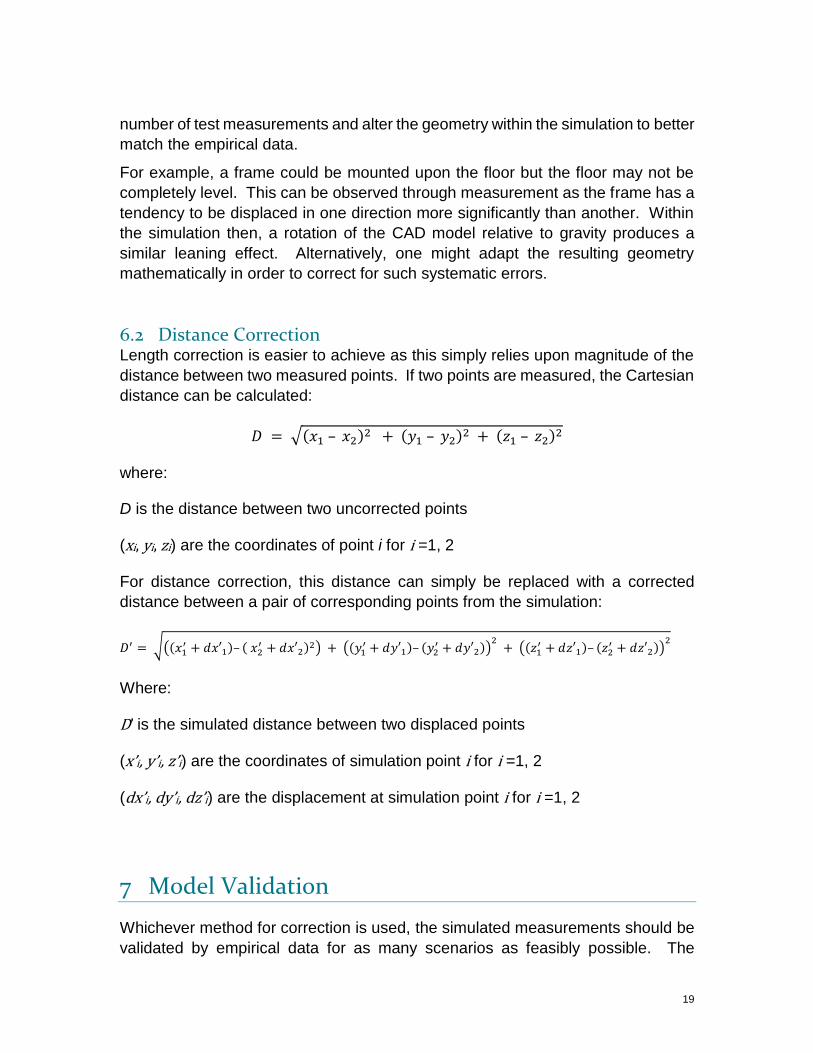
6.2 Distance Correction Length correction is easier to achieve as this simply relies upon magnitude of the

distance between two measured points. If two points are measured, the Cartesian

distance can be calculated:

𝐷 = √(𝑥1 – 𝑥2)2 + (𝑦1 – 𝑦2)2 + (𝑧1 – 𝑧2)2

where:

D is the distance between two uncorrected points

(xi, yi, zi) are the coordinates of point i for i =1, 2

For distance correction, this distance can simply be replaced with a corrected

distance between a pair of corresponding points from the simulation:

𝐷′ = √((𝑥1′ + 𝑑𝑥′1)– ( 𝑥2

′ + 𝑑𝑥′2)2) + ((𝑦1′ + 𝑑𝑦′1)– (𝑦2

′ + 𝑑𝑦′2))2

+ ((𝑧1′ + 𝑑𝑧′1)– (𝑧2

′ + 𝑑𝑧′2))2

Where:

D’ is the simulated distance between two displaced points

(x’i, y’i, z’i) are the coordinates of simulation point i for i =1, 2

(dx’i, dy’i, dz’i) are the displacement at simulation point i for i =1, 2

7 Model Validation

Whichever method for correction is used, the simulated measurements should be

validated by empirical data for as many scenarios as feasibly possible. The

20

selection of validation tests should be closely matched to the intended application

of the system.

Where the system needs to be used for very low uncertainty measurement, and is

likely to form part of a metrology solution that will be used a number of times, it

pays to spend as much time as possible in order to ensure that any simulation

results that are used to compensate measurements are as accurate as they can

be.

Whilst dimensional measurements are affected by temperature in different ways,

the best way to validate the simulation is to measure the object and compare this

to what the simulation predicts. These other thermal effects should be considered

when setting up such an experiment. Many instruments for large volume

metrology are optical, such as in the case of the laser tracker and photogrammetry

systems. As a result they are sensitive to anything in the environment that can

cause the refractive index along the optical path to change, causing the light to

bend through the air.

During the validation phase, it is permissible to use a more capable dimensional

measurement instrument than that which is to be used during normal operation, as

this phase is intended to be a measure of the simulation’s performance. For

temperature, however, it is important to use the sensors for validation that are to

be used in normal operation as these form your normal inputs to boundary

conditions. With that said, it is important to validate from a temperature

perspective also. During the validation phase, further sensors can be added as

passive observers whose readings are not be used as boundary conditions but

can identify areas where the thermal analysis is struggling to predict a fully

accurate temperature distribution. It may be that further sensors are needed to

inform the boundary conditions, or for existing sensors to be moved to a different

position. Any changes to the temperature sensor network feeding the boundary

conditions should prompt further validation of the simulation.

Robust prediction can be achieved by carrying out a range of tests within a normal

working range. But it is better still to be able to carry out some tests in which

conditions are more extreme than usual. This means that if for some reason an

extreme event does occur, the measurement corrections do not immediately need

to be discarded. It also means that more confidence can be vested in those

measurements that are taken in circumstances that are more likely to occur on a

more regular basis.

21

8 Uncertainty Evaluation

Thermal compensation can be beneficial to dimensional measurement but is not

without its own associated uncertainties. Uncertainties arise from a number of

sources in thermal compensation but can be generally be attributed to a

combination of physical measurement and modelling uncertainties.

Physical measurement uncertainty is a little more straightforward to evaluate, as

long as care is taken. Because the thermal compensation by its nature requires

that temperatures be measured and applied as boundary conditions, an

uncertainty budget needs to be produced to account for the sensors used. This is

not be discussed extensively here but further information can be found in the Guide

to the Expression of Uncertainty in Measurement (GUM) [21], other NPL Good

Practice Guides [7, 22], and a range of other sources.

Temperature sensors naturally vary in production, and drift can occur over time so

it is important to ensure sensors are regularly calibrated and tested.

The coefficient of thermal expansion (CTE) in materials can vary, which can make

large contributions to uncertainty. In some materials, CTE might vary by as much

as 10%. Whilst a number of materials have published properties, these cannot

necessarily be trusted as being absolute values for every sample of the same

material. Obtaining detailed material information with some measure of tolerance

from suppliers can go some way to remedy this. In some cases it may be possible

to carry out tests to verify the value is correct but this can be difficult in large scale

applications.

Uncertainty in simulation on the other hand can be a little more complicated, as

there are a number of variables to consider. This is largely a question of how

closely the simulation matches that which is to be modelled, and inherent

numerical errors resulting from solver calculations.

Software packages are available which can provide uncertainty quantification

using computational experiments. Demand for such software arose due to the

often ‘black box’ nature of some simulation solutions, where exactly what the

software is doing is not necessarily evident to the user. In addition, these packages

are also useful for design optimization, particularly in multi-parametric models.

These packages can interface with various CAE packages including CAD,

meshers and finite element analysis. OptiY [23], and modeFrontier [24] are

examples of packages that can be used for this purpose.

22

9 Acknowledgements

This work was funded by the EMRP Project IND53. The EMRP is funded by the

EMRP participating countries within EURAMET and the European Union. The

authors gratefully acknowledge this support and the help and encouragement of

all those involved.

10 Bibliography and Further Reading

[1] BSI. BS EN ISO 1. Geometrical product specifications (GPS). Standard reference temperature for the specification of geometrical and dimensional properties. BSI; 2015.

[2] Estler WT, Edmundson KL, Peggs GN, Parker DH. Large-Scale Metrology – An Update. CIRP Annals - Manufacturing Technology. 2002;51(2):587-609.

[3] Muelaner JE, Maropoulos PG, Large volume metrology technologies for the light controlled factory. Procedia CIRP Special Edition for 8th International Conference on Digital Enterprise Technology - DET 2014 – Disruptive Innovation in Manufacturing Engineering towards the 4th Industrial Revolution, DOI: 101016/jprocir201410026; 2014 25/03/2014 - 28/03/2014: Elsevier.

[4] Flack DH, J. Fundamental good practice in dimensional metrology. National Physical Laboratory, 2006 Contract No.: PDB: 4116.

[5] Auty FJ, Bevan, K, Hanson, A, Machin, G, Scott, J, Brown, C*, Haritos, G*, Martinez-Botas, R F*. Beginner's guide to measurement in mechanical engineering. National Physical Laboratory, 2014.

[6] Ross-Pinnock D. Integration of Thermal and Dimensional Measurement – A Hybrid Computational and Physical Measurement Method. 38th MATADOR Conference; 28-30th March 2015; Huwei, Taiwan: The University of Manchester; 2015. p. 471-8.

[7] Rusby R. Good Practice Guide No. 125. NPL Website: Queen’s Printer and Controller of HMSO; 2012. Available from: http://www.npl.co.uk/publications/guides/comment/beginners-guide-to-temperature-measurement/.

[8] Ross-Pinnock D, Maropoulos PG. Review of industrial temperature measurement technologies and research priorities for the thermal characterisation of the factories of the future. Proceedings of the Institution of Mechanical Engineers, Part B: Journal of Engineering Manufacture. 2015.

[9] Childs PRN, Greenwood JR, Long CA. Review of temperature measurement. Review of Scientific Instruments. 2000;71(8):2959-78.

23

[10] Ross-Pinnock D, Maropoulos PG, Identification of Key Temperature Measurement Technologies for the Enhancement of Product and Equipment Integrity in the Light Controlled Factory. Procedia CIRP Special Edition for 8th International Conference on Digital Enterprise Technology - DET 2014 – Disruptive Innovation in Manufacturing Engineering towards the 4th Industrial Revolution, DOI: 101016/jprocir201410019; 2014 25/03/2014 - 28/03/2014: Elsevier.

[11] Adams VA, A. Building Better Products with Finite Element Analysis. United States: OnWord Press; 1999.

[12] Moaveni S. Finite element analysis : theory and application with ANSYS. 2nd ed. ed. Upper Saddle River, N.J.: Upper Saddle River, N.J. : Pearson Education; 2003.

[13] Nakasone Y. Engineering analysis with ANSYS software. Burlington, MA : Butterworth-Heinemann; 2006.

[14] Pavlou DG. Essentials of the Finite Element Method For Mechanical and Structural Engineers. Burlington: Burlington : Elsevier Science; 2015.

[15] Lee H-H. Finite element simulations with ANSYS Workbench 13. Mission, Kan.: Mission, Kan. : Schroff Development Corporation; 2011.

[16] Megson THG. Structural and Stress Analysis. 2nd ed. ed. Burlington: Burlington : Elsevier Science; 2005.

[17] ANSYS. Explore Engineering Simulation: ANSYS; 2016 [cited 2016 13/07/16]. Available from: http://www.ansys.com/.

[18] Systèmes D. ABAQUS UNIFIED FEA: Dassault Systèmes; 2016 [cited 2016 13/07/16]. Available from: http://www.3ds.com/products-services/simulia/products/abaqus/.

[19] Corporation MS. MSC Nastran Multidisciplinary Structural Analysis 2015 [cited 2016 13/07/16]. Available from: http://www.mscsoftware.com/product/msc-nastran.

[20] Systemes D, Corporation S. Solidworks Products: Dassault Systemes, SolidWorks Corporation; 2016 [cited 2016 13/07/16]. Available from: http://www.solidworks.com/sw/3d-cad-design-software.htm.

[21] BIPM. Evaluation of Measurement Data - Guide to the expression of uncertainty in measurement. 2008.

[22] Cox MG, Dainton, M P, Harris, P M. Uncertainty and statistical modelling. National Physical Laboratory, 2001 Contract No.: PDB: 3472.

[23] GmbH O. CAD/CAE Design Technology for Reliability and Quality: OptiY GmbH; 2016 [cited 2016 13/07/2016]. Available from: http://www.optiy.eu/default.htm.

[24] ESTECO. modeFRONTIER: ESTECO; 2015 [cited 2016 13/07/16]. Available from: http://www.esteco.com/modefrontier.