62
Copyright © 2012 Pearson Education. Chapter 21 Design and Analysis of Experiments and Observational Studies
| Date post: | 28-Dec-2015 |
| Category: |
Documents |
| Upload: | sophia-page |
| View: | 222 times |
| Download: | 0 times |

Copyright © 2012 Pearson Education.
Chapter 21
Design and Analysisof Experiments and
Observational Studies

Copyright © 2012 Pearson Education. 21-2
21.1 Observational Studies
A statistical study is observational when it is conducted using pre-existing data—collected without any particular design.
Example: Many companies collect a variety of data via registration or warranty cards. This data might be utilized later in some observational study that seeks to discover correlations between the collected data.

Copyright © 2012 Pearson Education. 21-3
21.1 Observational Studies
An observational study is retrospective if it studies an outcome in the present by examining historical records.
An observational study is prospective if it seeks to identify subjects in advance and collects data as events unfold.
Example: Use credit card records to identify which customers earned the bank the most money, and then look for relationships in order to identify new customers with the same earning potential.
Example: Follow a sample of smokers and runners to discover the occurrence of emphysema.

Copyright © 2012 Pearson Education. 21-4
21.2 Randomized, ComparativeExperiments
An experiment is a study in which the experimenter manipulates attributes of what is being studied and observes the consequences.
The attributes, called factors, are manipulated by being set to particular levels and then allocated or assigned to individuals. An experimenter identifies at least one factor to manipulate and at least one response variable to measure.
The combination of factor levels assigned to a subject is called that subject’s treatment.

Copyright © 2012 Pearson Education. 21-5
21.2 Randomized, ComparativeExperiments
1) The experimenter actively and deliberately manipulates the factors to specify the treatment.
2) The experiment assigns the subjects to those treatments at random.
Two key features distinguish an experiment from other types of investigations.

Copyright © 2012 Pearson Education. 21-6
21.2 Randomized, ComparativeExperiments
Example: A soft-drink company wants to compare the formulas it has for their cola product. It created its cola with different types of sweeteners (sugar, corn syrup, and an artificial sweetener). All other ingredients and amounts were the same. Ten trained testers rated the colas on a scale of 1 to 10. The colas were presented to each taste tester in a random order.
Identify the experimental units, the treatments, the response, and the random assignment.
Experimental units: Colas
Treatments: Sweeteners
Response: Tester Rating
Random assignment: Colas were presented in a random order.

Copyright © 2012 Pearson Education. 21-7
21.3 The Four Principals of Experimental Design
1. Control
We control sources of variation other than the factors we are testing by making conditions as similar as possible for all treatment groups. An experimenter tries to make any other variables that are not manipulated as alike as possible.
Controlling extraneous sources of variation reduces the variability of the responses, making it easier to discern differences among the treatment groups.

Copyright © 2012 Pearson Education. 21-8
21.3 The Four Principals of Experimental Design
1. Control
There is a second meaning of control in experiments.
A bank testing the new creative idea of offering a card with special discounts on chocolate to attract more customers will want to compare its performance against one of its standard cards.
Such a baseline measurement is called a control treatment, and the group that receives it is called the control group.

Copyright © 2012 Pearson Education. 21-9
21.3 The Four Principals of Experimental Design
2. Randomize
In any true experiment, subjects are assigned treatments at random. Randomization allows us to equalize the effects of unknown or uncontrollable sources of variation. Although randomization can’t eliminate the effects of these sources, it spreads them out across the treatment levels so that we can see past them.
Randomization even protects us from effects we didn’t know about.

Copyright © 2012 Pearson Education. 21-10
21.3 The Four Principals of Experimental Design
3. Replicate
Because we need to estimate the variability of our measurements, we must make more than one observation at each level of each factor. Sometimes that just means making repeated observations. But, as we’ll see later some experiments combine two or more factors in ways that may permit a single observation for each treatment, that is, each combination of factor levels. When such an experiment is repeated in its entirety, it is said to be replicated. Repeated observations at each treatment are called replicates. If the number of replicates is the same for each treatment combination, we say that the experiment is balanced.

Copyright © 2012 Pearson Education. 21-11
21.3 The Four Principals of Experimental Design
3. Replicate
A second kind of replication is to repeat the entire experiment for a different group of subjects, under different circumstances, or at a different time.
Replication in a variety of circumstances can increase our confidence that our results apply to other situations and populations.

Copyright © 2012 Pearson Education. 21-12
21.3 The Four Principals of Experimental Design
4. Blocking
Group or block subjects together according to some factor that you cannot control and feel may affect the response. Such factors are called blocking factors, and their levels are called blocks.
Example blocking factors: sex, ethnicity, marital status, etc.
In effect, blocking an experiment into n blocks is equivalent to running n separate experiments.

Copyright © 2012 Pearson Education. 21-13
21.3 The Four Principals of Experimental Design
4. Blocking
Blocking in an experiment is like stratifying in a survey design. Blocking reduces variation by comparing subjects within these more homogenous groups. That makes it easier to discern any differences in response due to the factors of interest. In addition, we may want to study the effect of the blocking factor itself.
Blocking is an important compromise between randomization and control. However, unlike the first three principles, blocking is not required in all experiments.

Copyright © 2012 Pearson Education. 21-14
21.4 Experimental Designs
Completely Randomized Designs
When each of the possible treatments is assigned to at least one subject at random, the design is called a completely randomized design.
This design is the simplest and easiest to analyze of all experimental designs.

Copyright © 2012 Pearson Education. 21-15
21.4 Experimental Designs
Completely Randomized Designs
A diagram of the procedure can help in thinking about experiments. In this experiment the subjects are assigned at random to the different treatments. The simplest randomized design has two groups randomly assigned two different treatments.

Copyright © 2012 Pearson Education. 21-16
21.4 Experimental Designs
Randomized Block Designs
When one of the factors is a blocking factor, complete randomization isn’t possible. We can’t randomly assign factors based on people’s behavior, age, sex, and other attributes. But we may want to block by these factors in order to reduce variability and to understand their effect on the response.
When we have a blocking factor, we randomize the subject to the treatments within each block. This is called a randomized block design.

Copyright © 2012 Pearson Education. 21-17
21.4 Experimental Designs
Randomized Block Designs
In the following experiment, a marketer wanted to know the effect of two types of offers in each of two segments: a high spending group and a low spending group. The marketer selected 12,000 customers from each group at random and then randomly assigned the three treatments to the 12,000 customers in each group so that 4000 customers in each segment received each of the three treatments. A display makes the process clearer.

Copyright © 2012 Pearson Education. 21-18
21.4 Experimental Designs
Randomized Block Designs
This example of a randomized block design shows that customers are randomized to treatments within each segment, or block.

Copyright © 2012 Pearson Education. 21-19
21.4 Experimental Designs
Factorial Designs
An experiment with more than one manipulated factor is called a factorial design.
A full factorial design contains treatments that represent all possible combinations of all levels of all factors.
When the combination of two factors has a different effect than you would expect by adding the effects of the two factors together, that phenomenon is called an interaction.
If the experiment does not contain both factors, it is impossible to see interactions.

Copyright © 2012 Pearson Education. 21-20
21.4 Experimental Designs
Factorial Designs
It may seem that the added complexity of multiple factors is not worth the trouble. In fact, just the opposite is true. First, if each factor accounts for some of the variation in responses, having the important factors in the experiment makes it easier to discern the effects of each. Testing multiple factors in a single experiment makes more efficient use of the available subjects. And testing factors together is the only way to see what happens at combinations of the levels.

Copyright © 2012 Pearson Education. 21-21
21.5 Issues in Experimental Designs
Blinding and Placebos
Blinding: The deliberate withholding of the treatment details from individuals who might affect the outcome.
Two sources of unwanted bias:
Those who might influence the results (the subjects, treatment administrators, technicians, etc.)
Those who evaluate the results (judges, experimenters, etc.)
Single-Blind Experiment: one or the other groups is blinded.
Double-Blind Experiment: both groups are blinded.

Copyright © 2012 Pearson Education. 21-22
21.5 Issues in Experimental Designs
Blinding and Placebos
Often simply applying any treatment can induce an improvement. Some of the improvement seen with a treatment—even an effective treatment—can be due simply to the act of treating. To separate these two effects, we can sometimes use a control treatment that mimics the treatment itself. A “fake” treatment that looks just like the treatments being tested is called a placebo.
Placebos are the best way to blind subjects so they don’t know whether they have received the treatment or not.

Copyright © 2012 Pearson Education. 21-23
21.5 Issues in Experimental Designs
Confounding and Lurking Variables
When the levels of one factor are associated with the levels of another factor, we say that two factors are confounded.
Example: A bank offers credit cards with two possible treatments:
low rate & no fee high rate & $50 fee
There is no way to separate the effect of the rate factor from that of the fee factor. These two factors are confounded in this design.

Copyright © 2012 Pearson Education. 21-24
21.5 Issues in Experimental Designs
Confounding and Lurking Variables
Confounding variables seem somewhat like lurking variables. But, these two concepts are not the same.
• A lurking variable “drives” two other variables in such a way that a causal relationship is suggested between the two.
• Confounding occurs when levels incorporate more than one factor. The confounder does not necessarily “drive” the companion factor(s) in the level.
Copyright © 2012 Pearson Education. 21-25
21.5 Issues in Experimental Designs
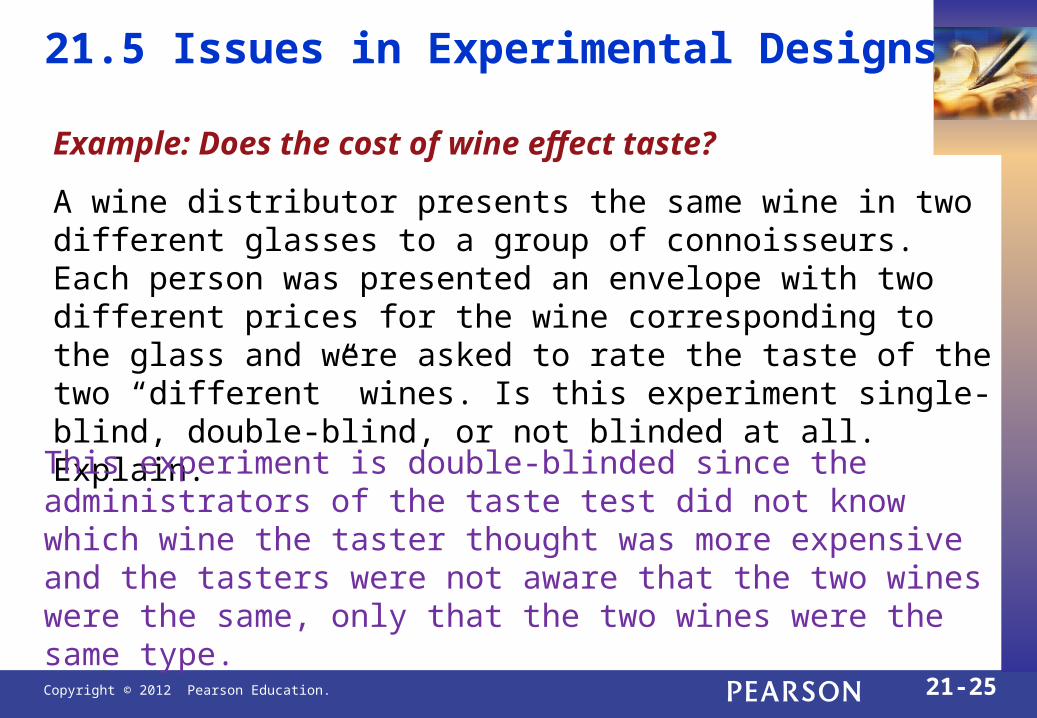
Example: Does the cost of wine effect taste?
A wine distributor presents the same wine in two different glasses to a group of connoisseurs. Each person was presented an envelope with two different prices for the wine corresponding to the glass and were asked to rate the taste of the two “different” wines. Is this experiment single-blind, double-blind, or not blinded at all. Explain.
This experiment is double-blinded since the administrators of the taste test did not know which wine the taster thought was more expensive and the tasters were not aware that the two wines were the same, only that the two wines were the same type.

Copyright © 2012 Pearson Education. 21-26
Let be the mean response for treatment group i.
21.6 Analyzing a Design in One Factor – The One-Way Analysis of Variance
Consider an experiment with a single factor of k levels.
Question of Primary Interest:
Is there evidence for differences in effectiveness for the treatments?
Then, to answer the question, we must test the hypothesis:
0 1 2:
: at least one mean is differentk
A
H
H
i
(no difference in treatments)
(at least one treatment has a different result)

Copyright © 2012 Pearson Education. 21-27
21.6 Analyzing a Design in One Factor– The One-Way Analysis of Variance
What criterion might we use to test the hypothesis?
The test statistic compares the variance of the means to what we’d expect that variance to be based on the variance of the individual responses. The differences among the means are the same for the two sets of boxplots, but it’s easier to see that they are different when the underlying variability is smaller.

Copyright © 2012 Pearson Education. 21-28
21.6 Analyzing a Design in One Factor– The One-Way Analysis of Variance
The F-statistic compares two measures of variation, called mean squares. The numerator measures the variation between the groups (treatments) and is called the Mean Square due to treatments (MST). The denominator measures the variation within the groups, and is called the Mean Square due to Error (MSE). The F-statistic is their ratio:
1,k N k
MSTF
MSE
Every F-distribution has two degrees of freedom, corresponding to the degrees of freedom for the mean square in the numerator and for the mean square (usually the MSE) in the denominator.

Copyright © 2012 Pearson Education. 21-29
21.6 Analyzing a Design in One Factor– The One-Way Analysis of Variance
1) The Mean Square due to Treatments (between-group variation measure)
2
1
1
mean for group
grand mean (mean of all the data)
observations in group
k
i ii
i
i
SSTMST
k
SST n y y
y i
y
n i
To quantify these two classes of variation, we introduce two new measures of variability for one-factor experiments with k levels:

Copyright © 2012 Pearson Education. 21-30
21.6 Analyzing a Design in One Factor– The One-Way Analysis of Variance
2) The Mean Square due to Error (within-group variation measure)
2
1
2
1
variance for group
observations in group
total number of observations
k
i ii
i
i
SSEMSE
N k
SSE n s
s i
n i
N

Copyright © 2012 Pearson Education. 21-31
21.6 Analyzing a Design in One Factor– The One-Way Analysis of Variance
This analysis is called an Analysis of Variance (ANOVA), but the hypothesis is actually about means. The null hypothesis is that the means are all equal. The collection of statistics—the sums of squares, mean squares, F-statistic, and P-value—are usually presented in a table, called the ANOVA table, like this one:

Copyright © 2012 Pearson Education. 21-32
21.6 Analyzing a Design in One Factor– The One-Way Analysis of Variance
Example: Tom’s Tom-Toms tries to boost catalog sales by offering one of four incentives with each purchase:
1) Free drum sticks
2) Free practice pad
3) Fifty dollars off any purchase
4) No incentive (control group)

Copyright © 2012 Pearson Education. 21-33
21.6 Analyzing a Design in One Factor– The One-Way Analysis of Variance
Here is a summary of the spending for the month after the start of the experiment. A total of 4000 offers were sent, 1000 per treatment.

Copyright © 2012 Pearson Education. 21-34
21.6 Analyzing a Design in One Factor– The One-Way Analysis of Variance
Use the summary data to construct an ANOVA table.
(This table is most often created using technology.)
•Since P is so small, we reject the null hypothesis and conclude that the treatment means differ.
•The incentives appear to alter the spending patterns.

Copyright © 2012 Pearson Education. 21-35
21.7 Assumptions and Conditionsfor ANOVA
Independence Assumption
The groups must be independent of each other.
No test can verify this assumption. You have to think about how the data were collected and check that the Randomization Condition is satisfied.

Copyright © 2012 Pearson Education. 21-36
21.7 Assumptions and Conditions for ANOVA
Equal Variance Assumption
ANOVA assumes that the true variances of the treatment groups are equal. We can check the corresponding Similar Variance Condition in various ways:
• Look at side-by-side boxplots of the groups. Look for differences in spreads.
• Examine the boxplots for a relationship between the mean values and the spreads. A common pattern is increasing spread with increasing mean.
• Look at the group residuals plotted against the predicted values (group means). See if larger predicted values lead to larger-magnitude residuals.

Copyright © 2012 Pearson Education. 21-37
21.7 Assumptions and Conditions for ANOVA
Normal Population Assumption
Like Student’s t-tests, the F-test requires that the underlying errors follow a Normal model. As before when we faced this assumption, we’ll check a corresponding Nearly Normal Condition.
• Examine the boxplots for skewness patterns.
• Examine a histogram of all the residuals.
• Example a Normal probability plot.

Copyright © 2012 Pearson Education. 21-38
21.7 Assumptions and Conditionsfor ANOVA
Normal Population Assumption
For the Tom’s Tom-Toms experiment, the residuals are not Normal. In fact, the distribution exhibits bimodality.

Copyright © 2012 Pearson Education. 21-39
21.7 Assumptions and Conditions for ANOVA
Normal Population Assumption
The bimodality shows up in every treatment!
This bimodality came as no surprise to the manager. He responded, “…customers …either order a complete new drum set, or…accessories… or choose not to purchase anything.”

Copyright © 2012 Pearson Education. 21-40
21.7 Assumptions and Conditionsfor ANOVA
Normal Population Assumption
These data (and the residuals) clearly violate the Nearly Normal Condition. Does that mean that we can’t say anything about the null hypothesis?
No. Fortunately, the sample sizes are large, and there are no individual outliers that have undue influence on the means. With sample sizes this large, we can appeal to the Central Limit Theorem and still make inferences about the means. In particular, we are safe in rejecting the null hypothesis.

Copyright © 2012 Pearson Education. 21-41
21.7 Assumptions and Conditionsfor ANOVA
Example: A test prep course
A tutoring organization says of the 20 students it worked with gained an average of 25 points on a given IQ test when they retook the test after the course.
Explain why this does not necessarily prove that the special course caused scores to go up.The students were not randomly assigned. Those who signed up for the course may be a special group whose scores would have improved anyway.
Design an experiment to test their claim
Give the IQ test to a group of volunteers and then randomly assign them to take the review course or to not take the review course. After a period of time re-administer the test.

Copyright © 2012 Pearson Education. 21-42
21.7 Assumptions and Conditions for ANOVA
Example: A test prep course
A tutoring organization says of the 20 students it worked with gained an average of 25 points on a given IQ test when they retook the test after the course.
It is suspected that the students with particularly low grades would benefit more from the course, how would you change your design to account for this suspicion.
After the initial test, group the volunteers based on their scores. Randomly assign half of each group to either take the review course or not. Compare the results from the two groups in the block design.

Copyright © 2012 Pearson Education. 21-43
*21.8 Multiple Comparisons
Knowing that the means differ leads to the question of which ones are different and by how much.
Methods that test these issues are called methods for multiple comparisons.
Question: Why don’t we simply use a t-test for differences between means to test each pair of group means?
Answer: Each t-test is subject to a Type I error, and the chances of committing such an error increase as the number of tested pairs increases.

Copyright © 2012 Pearson Education. 21-44
*21.8 Multiple Comparisons
The Bonferroni Method
Use the t-test methodology to test differences between the means, but use an inflated value for t* that lessens the accumulated chance of committing a Type I error by keeping the overall Type I error rate at or below This wider margin of error is called the minimum significant difference or MSD.• Let J represent the number of pairs of means.
• Then, find the confidence interval for each difference using the
confidence level instead of 1J
1 .
If a confidence interval does not contain 0, then a significant difference is indicated.
.

Copyright © 2012 Pearson Education. 21-45
*21.9 ANOVA on Observational Data
You can apply ANOVA to observational data if the boxplots show roughly equal spreads and symmetric, outlier-free distributions.
But, DO SO WITH CAUTION! These studies are prone to a variety of problems that are explicitly eliminated in well-designed experiments.
1) Observational studies are frequently unbalanced.
2) Randomization is usually absent.
3) There is no control over lurking variables or confounding variables.
4) Don’t draw causal conclusions even when the F-statistic is significant.

Copyright © 2012 Pearson Education. 21-46
21.10 Analysis of Multifactor DesignsDirect Mail Example
Two direct-mail factors are tested to examine their capacity to stimulate credit card spending:
1) Envelope logo design
Two levels: standard envelope, logo envelope
2) Frequent flyer miles rewards
Three levels: no offer, double miles, anywhere miles
30,000 mailings to 6 treatment groups of 5000 each

Copyright © 2012 Pearson Education. 21-47
21.10 Analysis of Multifactor DesignsDirect Mail Example
After 3 months:
Are there treatment effects? Use two-way ANOVA to analyze the data.

Copyright © 2012 Pearson Education. 21-48
21.10 Analysis of Multifactor DesignsDirect Mail Example
Two-Way ANOVA
Calculate five sums of squares (SS):
1) The total SS
2) The SS due to factor A (a levels)
3) The SS due to factor B (b levels)
4) The SS due to the interaction of A and B
5) The error SS

Copyright © 2012 Pearson Education. 21-49
21.10 Analysis of Multifactor DesignsDirect Mail Example
Technology is used to generate a two-way ANOVA table:
There are 3 null hypotheses for two-way ANOVA:
1) The means of levels for factor A are equal.
2) The mean of levels for factor B are equal.
3) The effects of factor A are constant across the levels of factor B (no interaction between A and B).

Copyright © 2012 Pearson Education. 21-50
21.10 Analysis of Multifactor DesignsDirect Mail Example
Here is the ANOVA table for the direct mailing study:
• Both Miles and Envelope are highly significant.
• The interaction between Miles and Envelopes is not significant.

Copyright © 2012 Pearson Education. 21-51
21.10 Analysis of Multifactor DesignsDirect Mail Example
Use an interaction plot to visualize the effects and the interaction:
• The points show the effect of the levels of both Miles and Envelope.
• The fact that the two “lines” are parallel shows that there is little interaction.

Copyright © 2012 Pearson Education. 21-52
21.10 Analysis of Multifactor Designs
Two-Way ANOVA: Formulas
Un-replicated Design (one observation per group)
2 2
1 1 1
1
a b a
i ii j i
SSA b y y y y
SSAMSA
a
Factor A:
Factor B: 2 2
1 1 1
1
b a b
j jj i j
SSB a y y y y
SSBMSB
b

Copyright © 2012 Pearson Education. 21-53
21.10 Analysis of Multifactor Designs
Two-Way ANOVA: Formulas
Un-replicated Design (one observation per group)
2
1 1
1
a b
iji j
SSE SSTotal SSA SSB
SSTotal y y
SSEMSE
N a b
N a b
Error:

Copyright © 2012 Pearson Education. 21-54
21.10 Analysis of Multifactor Designs
Two-Way ANOVA: Formulas
Un-replicated Design (one observation per group)
1, 1
1, 1
a N a b
b N a b
MSAF
MSEMSB
FMSE
There are two F-statistics:
Copyright © 2012 Pearson Education. 21-55
21.10 Analysis of Multifactor Designs
Two-Way ANOVA: Formulas
Balanced Replicated Design (r observation(s) per group)
22
1 1 1 1 1 1
and r b a r a b
i jk j i k i j
SSA y y SSB y y
Interaction sum of squares:
2
1 1 1
1 1
r b a
ij i jk j i
SSAB y y y y
SSABMSAB
a b

Copyright © 2012 Pearson Education. 21-56
21.10 Analysis of Multifactor Designs
Two-Way ANOVA: Formulas
Balanced Replicated Design (r observation(s) per group)
2
1 1 1
1
r b a
ijk ijk j i
SSE y y
SSEMSE
ab r
There are three F-statistics:
1, 1 1, 1 1 1 , 1, , a ab r b ab r a b ab r
MSA MSB MSABF F F
MSE MSE MSE

Copyright © 2012 Pearson Education. 21-57
• Don’t give up just because you can’t run an experiment.
• Beware of confounding.
• Bad things can happen even to good experiments.
• Don’t spend your entire budget on the first run.
• Watch out for outliers.
• Watch out for changing variances.

Copyright © 2012 Pearson Education. 21-58
• Be wary of drawing conclusions about causality from observational studies.
• Be wary of generalizing to situations other than the one at hand.
• Watch for multiple comparisons.
• Be sure to fit an interaction term when it exists.
• When the interaction effect is significant, don’t interpret the main effects.

Copyright © 2012 Pearson Education. 21-59
What Have We Learned?
Recognize observational studies.
• A retrospective study looks at an outcome in the present and looks for facts in the past that relate to it.
• A prospective study selects subjects and follows them as events unfold.
Know the elements of a designed randomized experiment.
• Experimental units (sometimes called subjects or participants) are assigned at random to treatments.
• A quantitative response variable is measured or observed for each experimental unit.
• We can attribute differences in the response to the differences among treatments.

Copyright © 2012 Pearson Education. 21-60
What Have We Learned?
State and apply the Four Principles of Experimental Design.
• Control sources of variation other then the factors being tested. Make the conditions as similar as possible for all treatment groups except for the differences among the treatments.
• Randomize the assignment of subjects to treatments. Balance the design by assigning the same number of subjects to each treatment.
• Replicate the experiment on more than one subject.
• Block the experiment by grouping together subjects who are similar in important ways that you cannot control.

Copyright © 2012 Pearson Education. 21-61
What Have We Learned?
Work with blinding and control groups.
• A single-blind study is one in which either all who can affect the results or all those who evaluate the results are kept ignorant of which subjects receive which treatments.
• A double-blind study is one in which both those classes of actors are ignorant of the treatment assignment.
• A control group is assigned to a null treatment or to the best available alternative treatment. Control subjects are often administered a placebo or a null treatment that mimics the treatment being studied but is known to be inactive.

Copyright © 2012 Pearson Education. 21-62
What Have We Learned?
Understand how to use Analysis of Variance (ANOVA) to analyze designed experiments.
• ANOVA tables follow a standard layout; be acquainted with it.
• The F-statistic is the test statistic used in ANOVA. F-statistics test hypotheses about the equality of the means of two groups.
The Bonferroni Method is for identifying which treatments are different.


