Experiments & Observational Studies:

Causal Inference in Statistics

Paul R. Rosenbaum

Department of Statistics

University of Pennsylvania

Philadelphia, PA 19104-6340

1 My Concept of a ‘Tutorial’

• In the computer era, we often receive compressedfiles, .zip. Minimize redundancy, minimize storage,at the expense of intelligibility.

• Sometimes scientific journals seemed to have beencompressed.

• Tutorial goal is: ‘uncompress’. Make it possible toread a current article or use current software withoutgoing back to dozens of earlier articles.

2 A Causal Question

• At age 45, Ms. Smith is diagnosed with stage IIbreast cancer.

• Her oncologist discusses with her two possible treat-ments: (i) lumpectomy alone, or (ii) lumpectomyplus irradiation. They decide on (ii).

• Ten years later, Ms. Smith is alive and the tumorhas not recurred.

• Her surgeon, Steve, and her radiologist, Rachael de-bate.

• Rachael says: “The irradiation prevented the recur-rence – without it, the tumor would have recurred.”

• Steve says: “You can’t know that. It’s a fantasy –you’re making it up. We’ll never know.”

3 Many Causal Questions

• Steve and Rachael have this debate all the time.About Ms. Jones, who had lumpectomy alone. AboutMs. Davis, whose tumor recurred after a year.

• Whenever a patient treated with irradiation remainsdisease free, Rachael says: “It was the irradiation.”Steve says: “You can’t know that. It’s a fantasy.We’ll never know.”

• Rachael says: “Let’s keep score, add ’em up.” Stevesays: “You don’t know what would have happenedto Ms. Smith, or Ms. Jones, or Ms Davis – youjust made it all up, it’s all fantasy. Common sensesays: ‘A sum of fantasies is total fantasy.’ Commonsense says: ‘You can’t add fantasies and get facts.’Common sense says: ‘You can’t prove causality withstatistics.’”

4 Fred Mosteller’s Comment

• Mosteller like to say: “You can only prove causalitywith statistics.”

• He was thinking about a particular statistical methodand a particular statistician.

• Not Gauss and least squares, or Yule and Yule’s Q(a function of the odds ratio), or Wright and pathanalysis, or Student and the t-test.

• Rather, Sir Ronald Fisher and randomized experi-ments.

5 Fisher & Randomized Experiments

• Fisher’s biographer (and daughter) Joan Fisher Box(1978, p. 147) suggests that Fisher invented ran-domized experiments around 1920, noting that hispaper about ANOVA in experiments of 1918 madeno reference to randomization, referring to Normaltheory instead, but by 1923, his papers used ran-domization, not Normal theory, as the justificationfor ANOVA.

• Fisher’s clearest and most forceful discussion of ran-domization as ‘the reasoned basis for inference’ inexperiments came in his book of 1935, Design ofExperiments.

6 15 Pages

• In particular, the 15 pages of Chapter 2 discuss whatcame to be known as Fisher’s exact test for a 2× 2table. The hypergeometric distribution is dispatchedin half a paragraph, and Fisher hammers away inEnglish for 1412 pages about something else.

• Of Fisher’s method of randomization and randomiza-tion, Yule would write: “I simply cannot make heador tail of what the man is doing.” (Box 1978, p.150). But Neyman (1942, p. 311) would describeit as “a very brilliant method.”

7 Lumpectomy and Irradiation

• Actually, Rachael was right, Steve was wrong. Per-haps not in every case, but in many cases. Theaddition of irradiation to lumpectomy causes thereto be fewer recurrences of breast cancer.

• On 17 October 2002, the New England Journal ofMedicine published a paper by Bernard Fisher, et al.describing 20 year follow-up of a randomized trialcomparing lumpectomy alone and lumpectomy plusirradiation.

• There were 634 women randomly assigned to lumpec-tomy, 628 to lumpectomy plus irradiation.

• Over 20 years of follow-up, 39% of those who hadlumpectomy alone had a recurrence of cancer, asopposed to 14% of those who had lumpectomy plusirradiation (P<0.001).

8 Outline: Causal Inference

. . . in randomized experiments.

¥ Causal effects. ¥ Randomization tests of no effect.¥ Inference about magnitudes of effect.

. . . in observational studies.

¥ What happens when randomized experiments are notpossible? ¥ Adjustments for overt biases: How to doit. When does it work or fail. ¥ Sensitivity to hiddenbias. ¥ Reducing sensitivity to hidden bias.

9 Finite Population

• In Fisher’s formulation, randomization inference con-cerns a finite population of n subjects, the n subjectsactually included in the experiment, i = 1, . . . , n.

• Say n = 1, 262, in the randomized experiment com-paring lumpectomy (634) vs lumpectomy plus irra-diation (628).

• The inference is not to some other population. Theinference is to how these n people would have re-sponded under treatments they did not receive.

• We are not sampling people. We are sampling pos-sible futures for n fixed people.

• Donald Campbell would emphasize the distinctionbetween internal and external validity.

10 Causal Effects: Potential Out-comes

• Key references: Neyman (1923), Rubin (1974).

• Each person i has two potential responses, a re-sponse that would be observed under the ‘treatment’condition T and a response that would be observedunder the ‘control’ condition C.

rTi =

1 if woman i would have cancerrecurrence with lumpectomy alone0 if woman i would not have cancerrecurrence with lumpectomy alone

rCi =

1 if woman i would have cancerrecurrence with lumpectomy+irradiation0 if woman i would not have cancerrecurrence with lumpectomy+irradiation

• We see rTi or rCi, but never both. For Ms. Smith,we saw rCi.

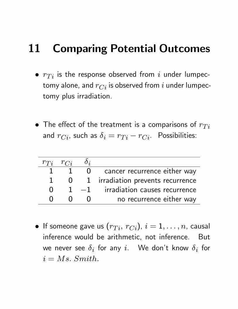
11 Comparing Potential Outcomes

• rTi is the response observed from i under lumpec-tomy alone, and rCi is observed from i under lumpec-tomy plus irradiation.

• The effect of the treatment is a comparisons of rTiand rCi, such as δi = rTi − rCi. Possibilities:

rTi rCi δi1 1 0 cancer recurrence either way1 0 1 irradiation prevents recurrence0 1 −1 irradiation causes recurrence0 0 0 no recurrence either way

• If someone gave us (rTi, rCi), i = 1, . . . , n, causalinference would be arithmetic, not inference. Butwe never see δi for any i. We don’t know δi fori =Ms. Smith.

12 Recap

• A finite population of n = 1, 262 women.

• Each woman has two potential responses, (rTi, rCi),but we see only one of them. Never see δi =

rTi − rCi, i = 1, . . . , n.

• Is it plausible that irradiation does nothing? Nullhypothesis of no effect. H0 : δi = 0, i = 1, . . . , n.

• Estimate the average treatment effect: 1nPni=1 δi.

• How many more women did not have a recurrence ofcancer because they received irradiation? (Attribut-able effect)

• The (rTi, rCi) are 2n fixed numbers describing thefinite population. Nothing is random.

13 Fisher’s Idea: Randomization

• Randomization converts impossible arithmetic intofeasible statistical inference.

• Pick m of the n people at random and give themtreatment condition T . In the experiment, m =634, n = 1, 262. That is, assign treatments

“in a random order, that is in an order not deter-mined arbitrarily by human choice, but by theactual manipulation of the physical apparatusused in games of chance, cards, dice, roulettes,etc., or, more expeditiously, from a publishedcollections of random sampling numbers. . . ” (Fisher,1935, Chapter 2)

• This means that each of the³nm

´=³1,262634

´treat-

ment assignments has the same probability,³1,262634

´−1.

The only probabilities that enter Fisher’s randomiza-tion inference are created by randomization.

14 Observable Quantities

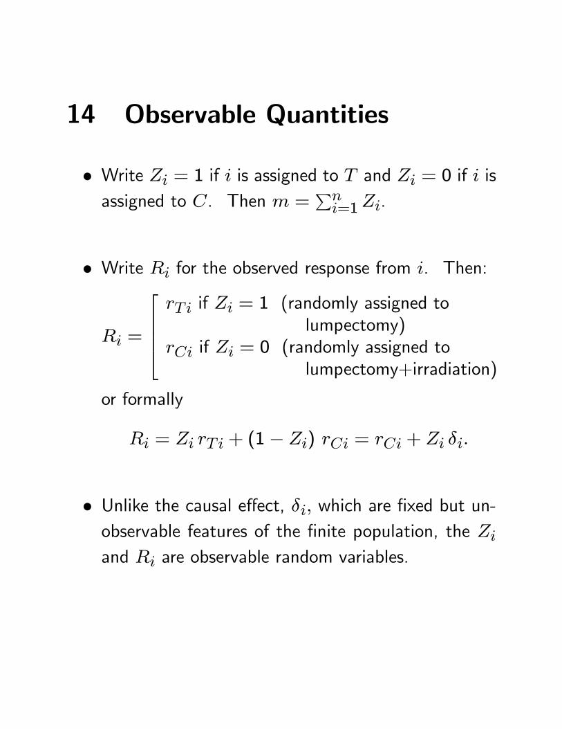
• Write Zi = 1 if i is assigned to T and Zi = 0 if i isassigned to C. Then m =

Pni=1Zi.

• Write Ri for the observed response from i. Then:

Ri =

rTi if Zi = 1 (randomly assigned to

lumpectomy)rCi if Zi = 0 (randomly assigned to

lumpectomy+irradiation)

or formally

Ri = Zi rTi + (1− Zi) rCi = rCi + Zi δi.

• Unlike the causal effect, δi, which are fixed but un-observable features of the finite population, the Ziand Ri are observable random variables.

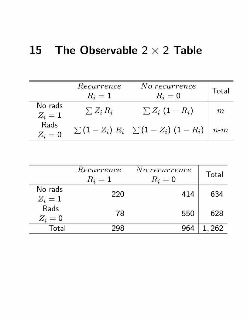
15 The Observable 2× 2 Table

RecurrenceRi = 1

No recurrenceRi = 0

Total

No radsZi = 1

PZi Ri

PZi (1−Ri) m

RadsZi = 0

P(1− Zi) Ri

P(1− Zi) (1−Ri) n-m

RecurrenceRi = 1

No recurrenceRi = 0

Total

No radsZi = 1

220 414 634

RadsZi = 0

78 550 628

Total 298 964 1, 262

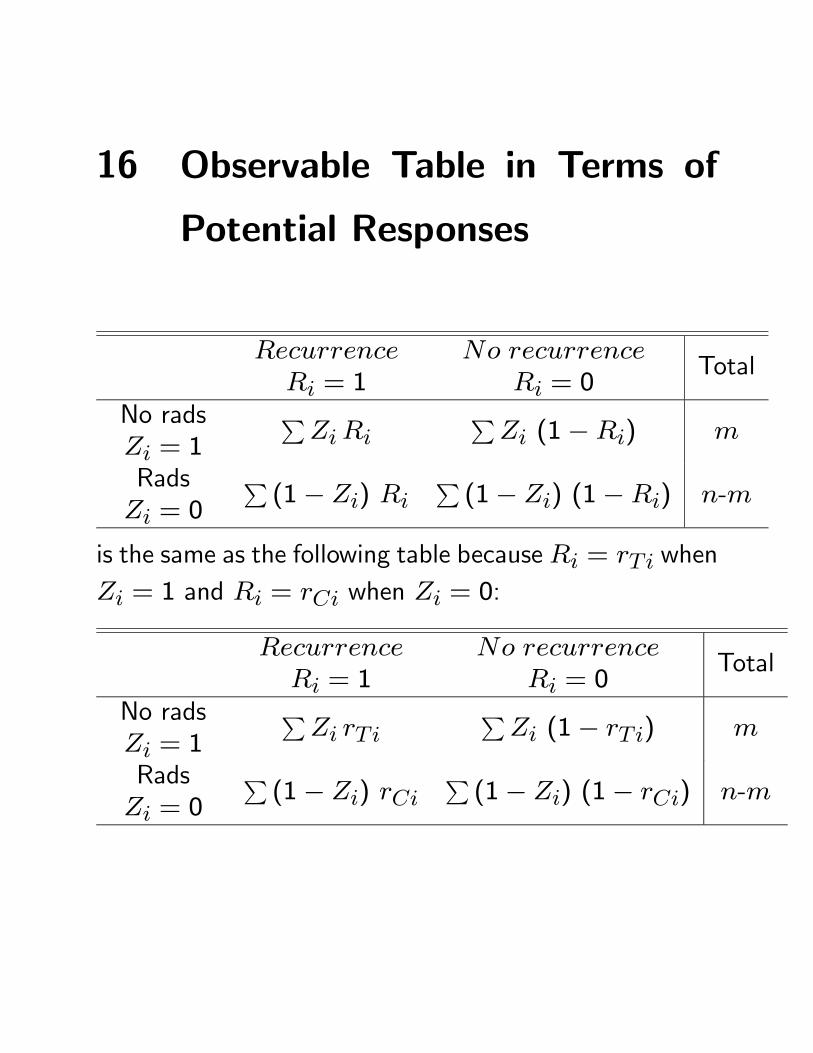
16 Observable Table in Terms of

Potential Responses

RecurrenceRi = 1

No recurrenceRi = 0

Total

No radsZi = 1

PZi Ri

PZi (1−Ri) m

RadsZi = 0

P(1− Zi) Ri

P(1− Zi) (1−Ri) n-m

is the same as the following table becauseRi = rTi whenZi = 1 and Ri = rCi when Zi = 0:

RecurrenceRi = 1

No recurrenceRi = 0

Total

No radsZi = 1

PZi rTi

PZi (1− rTi) m

RadsZi = 0

P(1− Zi) rCi

P(1− Zi) (1− rCi) n-m

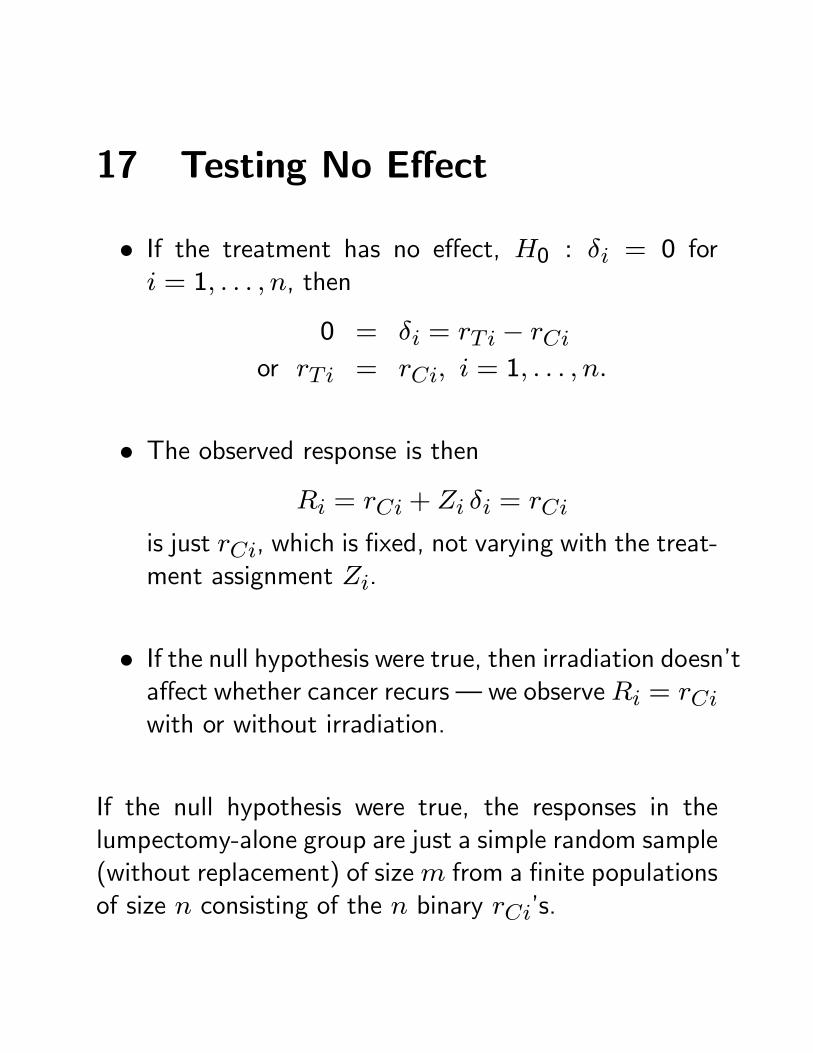
17 Testing No Effect

• If the treatment has no effect, H0 : δi = 0 fori = 1, . . . , n, then

0 = δi = rTi − rCior rTi = rCi, i = 1, . . . , n.

• The observed response is thenRi = rCi + Zi δi = rCi

is just rCi, which is fixed, not varying with the treat-ment assignment Zi.

• If the null hypothesis were true, then irradiation doesn’taffect whether cancer recurs – we observeRi = rCiwith or without irradiation.

If the null hypothesis were true, the responses in thelumpectomy-alone group are just a simple random sample(without replacement) of sizem from a finite populationsof size n consisting of the n binary rCi’s.

18 2 × 2 Table Under No effect:

Fisher’s Exact Test

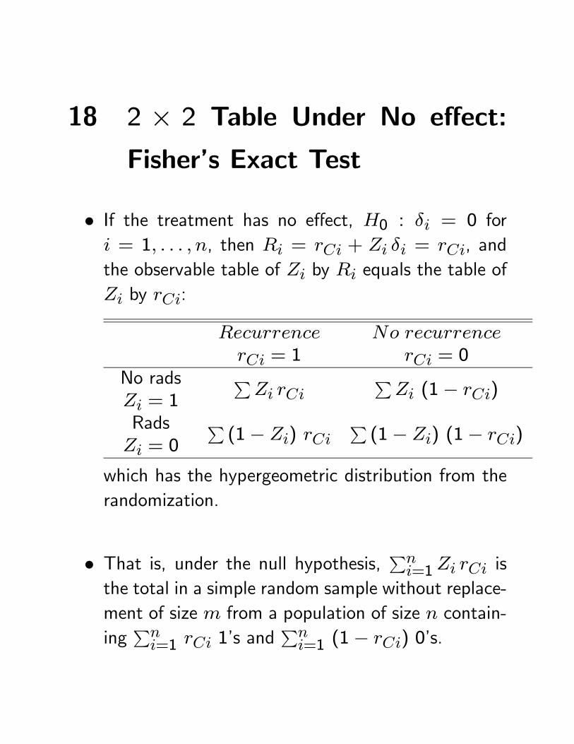
• If the treatment has no effect, H0 : δi = 0 fori = 1, . . . , n, then Ri = rCi + Zi δi = rCi, andthe observable table of Zi by Ri equals the table ofZi by rCi:

RecurrencerCi = 1

No recurrencerCi = 0

No radsZi = 1

PZi rCi

PZi (1− rCi)

RadsZi = 0

P(1− Zi) rCi

P(1− Zi) (1− rCi)

which has the hypergeometric distribution from therandomization.

• That is, under the null hypothesis, Pni=1Zi rCi is

the total in a simple random sample without replace-ment of size m from a population of size n contain-ing

Pni=1 rCi 1’s and

Pni=1 (1− rCi) 0’s.

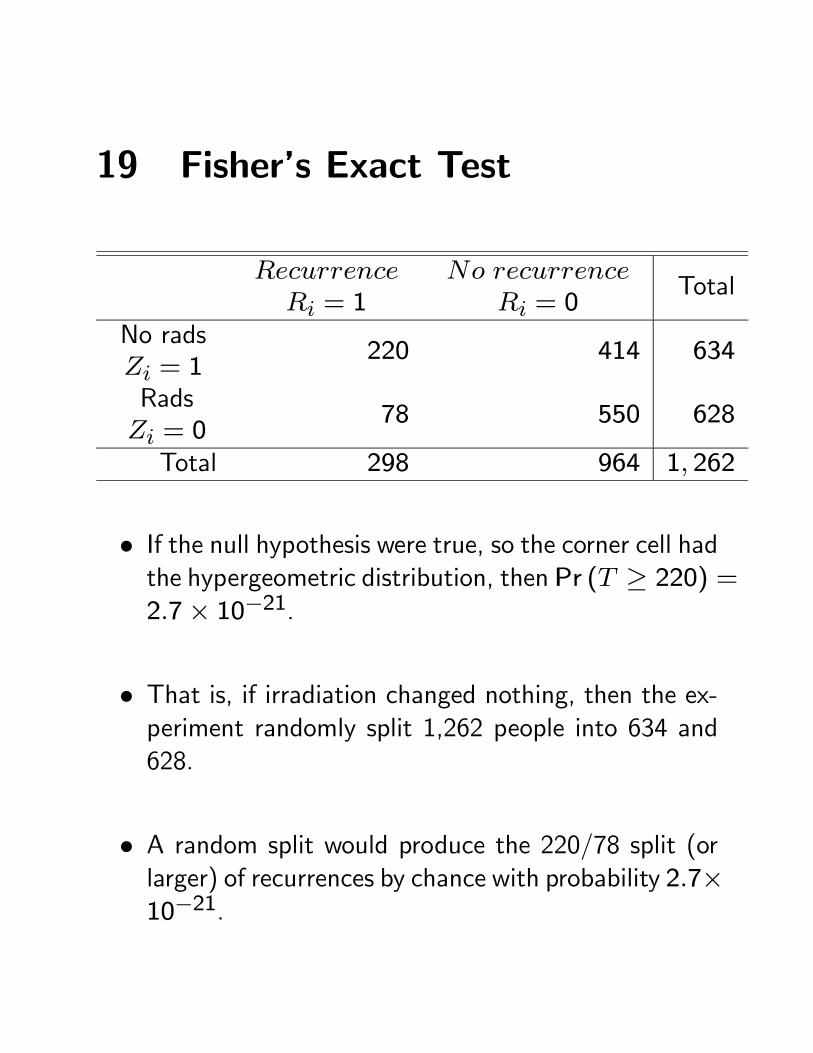
19 Fisher’s Exact Test

RecurrenceRi = 1

No recurrenceRi = 0

Total

No radsZi = 1

220 414 634

RadsZi = 0

78 550 628

Total 298 964 1, 262

• If the null hypothesis were true, so the corner cell hadthe hypergeometric distribution, then Pr (T ≥ 220) =2.7× 10−21.

• That is, if irradiation changed nothing, then the ex-periment randomly split 1,262 people into 634 and628.

• A random split would produce the 220/78 split (orlarger) of recurrences by chance with probability 2.7×10−21.

20 How far have we come?

• We never see any causal effects, δi.

• Yet we are 100³1− 2.7× 10−21

´% confident that

some δi > 0.

• Causal inference is impossible at the level of an in-dividual, i, but it is straightforward for a populationof n individuals if treatments are randomly assigned.

• Mosteller’s comment: “You can only prove causalitywith statistics.”

21 Testing other hypotheses

• Recall that δi = rTi − rCi, and Fisher’s exact testrejected H0 : δi = 0, i = 1, . . . , n = 1262.

• Consider testing insteadH0 : δi = δ0i, i = 1, . . . , n =1262 with the δ0i as possible specified values of δi.

• Since Ri = rCi + Zi δi, if the hypothesis H0 weretrue, then Ri − Zi δ0i would equal rCi.

• But Ri and Zi are observed and δ0i is specified bythe hypothesis, so if the hypothesis were true, wecould calculate the rCi.

• Under the null hypothesis, the 2 × 2 table record-ing rCi by Zi has the hypergeometric distribution,yielding a test.

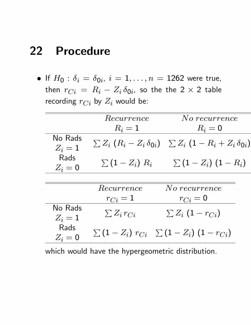
22 Procedure

• If H0 : δi = δ0i, i = 1, . . . , n = 1262 were true,then rCi = Ri − Zi δ0i, so the the 2 × 2 tablerecording rCi by Zi would be:

RecurrenceRi = 1

No recurrenceRi = 0

No RadsZi = 1

PZi (Ri − Zi δ0i)

PZi (1−Ri + Zi δ0i)

RadsZi = 0

P(1− Zi) Ri

P(1− Zi) (1−Ri)

RecurrencerCi = 1

No recurrencerCi = 0

No RadsZi = 1

PZi rCi

PZi (1− rCi)

RadsZi = 0

P(1− Zi) rCi

P(1− Zi) (1− rCi)

which would have the hypergeometric distribution.

23 Attributable effect

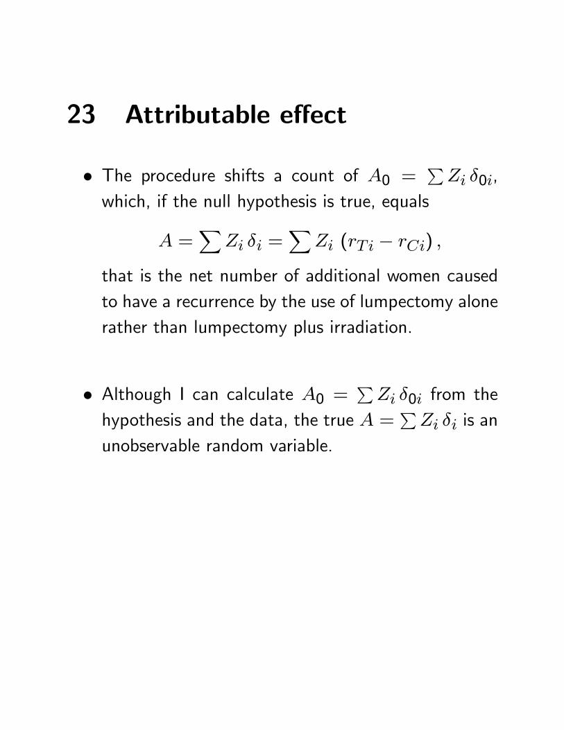
• The procedure shifts a count of A0 =PZi δ0i,

which, if the null hypothesis is true, equals

A =X

Zi δi =X

Zi (rTi − rCi) ,

that is the net number of additional women causedto have a recurrence by the use of lumpectomy alonerather than lumpectomy plus irradiation.

• Although I can calculate A0 =PZi δ0i from the

hypothesis and the data, the true A =PZi δi is an

unobservable random variable.

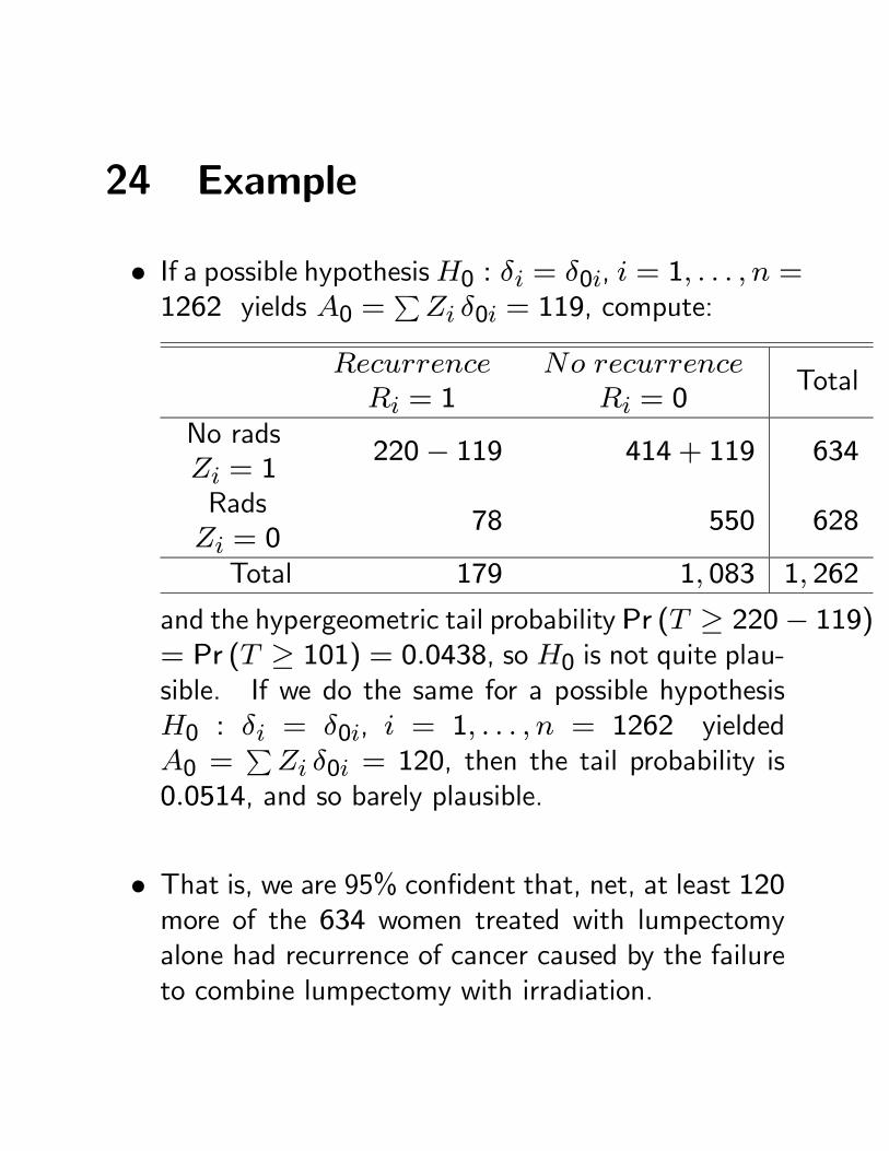
24 Example

• If a possible hypothesisH0 : δi = δ0i, i = 1, . . . , n =1262 yields A0 =

PZi δ0i = 119, compute:

RecurrenceRi = 1

No recurrenceRi = 0

Total

No radsZi = 1

220− 119 414 + 119 634

RadsZi = 0

78 550 628

Total 179 1, 083 1, 262

and the hypergeometric tail probability Pr (T ≥ 220− 119)= Pr (T ≥ 101) = 0.0438, so H0 is not quite plau-sible. If we do the same for a possible hypothesisH0 : δi = δ0i, i = 1, . . . , n = 1262 yieldedA0 =

PZi δ0i = 120, then the tail probability is

0.0514, and so barely plausible.

• That is, we are 95% confident that, net, at least 120more of the 634 women treated with lumpectomyalone had recurrence of cancer caused by the failureto combine lumpectomy with irradiation.

25 Randomization Inference in Gen-eral

• Randomization inference was illustrated in a simplesituation: Fisher’s exact test for a 2× 2 table.

• The concept is very general, however. Among thetests commonly derived as randomization tests are:Wilcoxon’s signed rank and rank sum tests, the Mantel-Haenszel-Birch test for 2×2×S tables, the Mantel-extension test for integer scores, the Gehan and log-rank tests for censored survival data. (eg Lehmann1999)

• In a randomized experiment, ANOVA-based tests canbe derived as approximations to randomization tests.(eg. Welch 1937).

• Can be combined with models (Gail, et al 1988),smoothers (Raz 1990), and nonparametric covari-ance adjustments (Rosenbaum 2002).

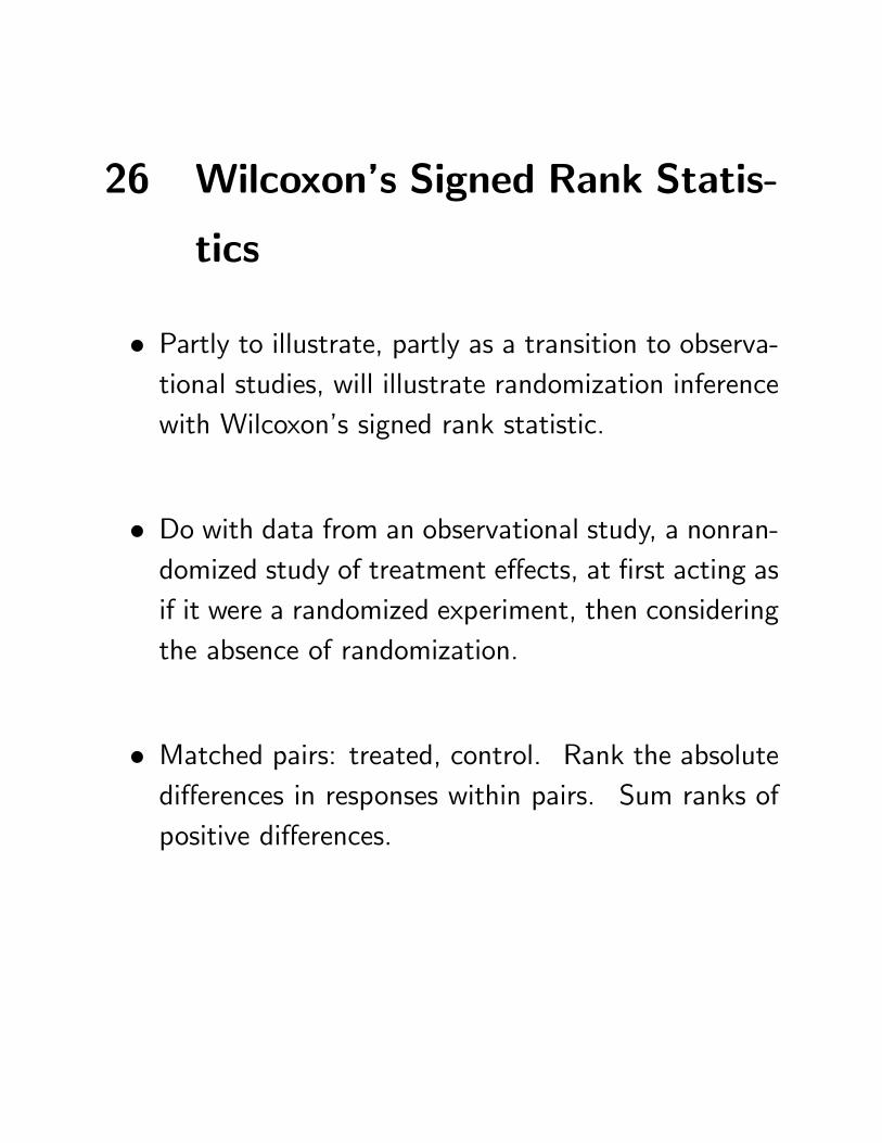
26 Wilcoxon’s Signed Rank Statis-

tics

• Partly to illustrate, partly as a transition to observa-tional studies, will illustrate randomization inferencewith Wilcoxon’s signed rank statistic.

• Do with data from an observational study, a nonran-domized study of treatment effects, at first acting asif it were a randomized experiment, then consideringthe absence of randomization.

• Matched pairs: treated, control. Rank the absolutedifferences in responses within pairs. Sum ranks ofpositive differences.

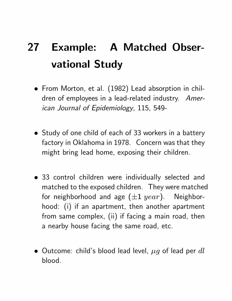
27 Example: A Matched Obser-vational Study

• From Morton, et al. (1982) Lead absorption in chil-dren of employees in a lead-related industry. Amer-ican Journal of Epidemiology, 115, 549-

• Study of one child of each of 33 workers in a batteryfactory in Oklahoma in 1978. Concern was that theymight bring lead home, exposing their children.

• 33 control children were individually selected andmatched to the exposed children. They were matchedfor neighborhood and age (±1 year). Neighbor-hood: (i) if an apartment, then another apartmentfrom same complex, (ii) if facing a main road, thena nearby house facing the same road, etc.

• Outcome: child’s blood lead level, µg of lead per dlblood.

28 Notation for a Paired Experi-

ment

Pair s, Subject i: S = 33 pairs, s = 1, . . . , S = 33,with 2 subjects in each pair, i = 1, 2.

One treated, one control in each pair: WriteZsi =1 if the ith subject in pair s is treated, Zsi = 0 ifcontrol, so Zs1 + Zs2 = 1 for every s, or Zs2 =1− Zs1. For all 2S subjects,

Z = (Z11, Z12, . . . , ZS1, ZS2)T .

Random assignment of treatments within pairs: Ω

is the set of the K = 2S possible values z of Z, andrandomization picks one of these at random,

Pr (Z = z) =1

Kfor each z ∈ Ω.

2040

60

Exposed Control

Bloo

d Le

ad, m

icro

gram

s/dl

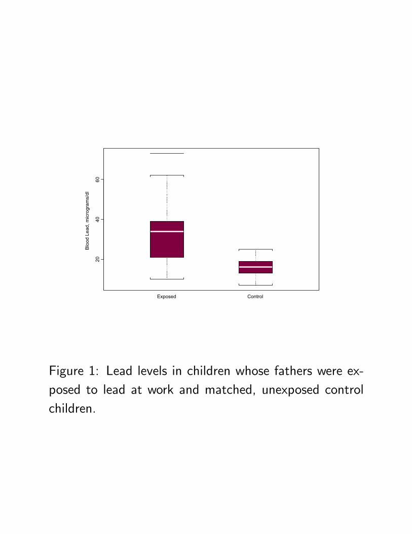
Figure 1: Lead levels in children whose fathers were ex-posed to lead at work and matched, unexposed controlchildren.

020

4060

Exposed-Control

Diff

eren

ce in

Blo

od L

ead

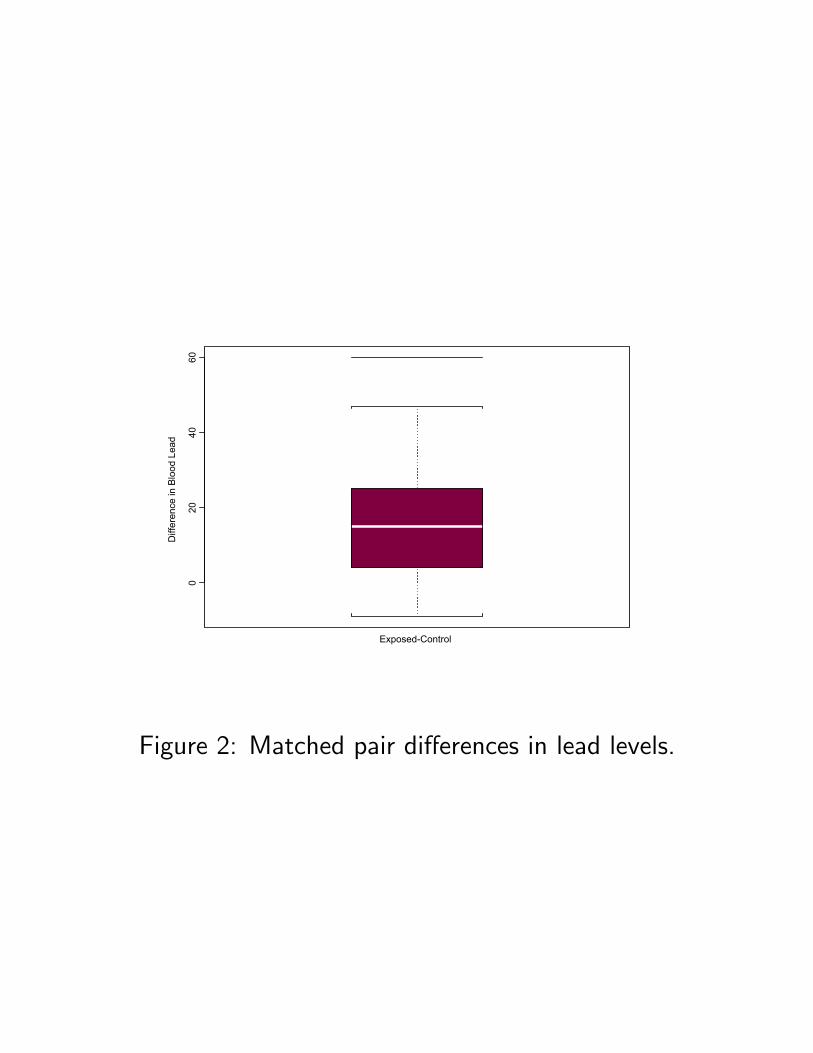
Figure 2: Matched pair differences in lead levels.

29 Responses, Causal Effects

Potential responses, causal effects, as before. Eachof the 2S subjects (s, i) has two potential responses,a response rTsi that would be seen under treat-ment and a response rCsi that would be seen un-der control. (Neyman 1923, Rubin 1974). Treat-ment effect is δsi = rTsi − rCsi. Additive effect,rTsi − rCsi = τ or δsi = τ for all s, i.

Finite population, as before. The (rTsi, rCsi) , s =1, . . . , S, i = 1, 2, are again fixed features of thefinite population of 2S subjects.

Observed responses, as before. Observed responseis Rsi = rTsi if Zsi = 1 or Rsi = rCsi if Zsi = 0,that is, Rsi = Zsi rTsi+ (1− Zsi) rCsi = rCsi+Zsi δsi. If effect is additive, Rsi = rCsi + Zsi τ .

Vectors. 2S−dimensional vectors rT , rC, δ, R; e.g.,R = (R11, . . . , RS2)

T .

30 Treated-Minus-Control Differences

Who is treated in pair s? If Zs1 = 1, then (s, 1) istreated and (s, 2) is control, but if Zs2 = 1 then(s, 2) is treated and (s, 1) is control.

Treated-minus-control differences with additive effects:If rTsi − rCsi = τ , then a little algebra showsthe treated-minus-control difference in observed re-sponses in pair s is:

Ds = (Zs1 − Zs2) (rCs1 − rCs2) + τ.

In general, without additive effects: In general, withδsi = rTsi − rCsi:

Ds = (Zs1 − Zs2) (rCs1 − rCs2)+Zs1 δs1+Zs2 δs2.

31 Signed Rank Statistic

Usual form. Wilcoxon’s signed rank statistic W ranksthe |Ds| from 1 to S, and sums the ranks of thepositive Ds. (Ties ignored today.)

Equivalent alternative form. Another expression forW uses the S (S + 1) /2 Walsh averages,

Ds +Ds02

, with 1 ≤ s ≤ s0 ≤ S;

then W is the number of positive Walsh averages.(Lehmann 1998)

Offsets. A Walsh average (Ds +Ds0) /2 is positive ifthe more affected pair of s and s0 was sufficientlyaffected to offset whatever happened to the less af-fected pair, that is, if max (Ds,Ds0) is sufficientlylarge that it averages with min (Ds,Ds0) to be pos-itive. Then W is the number of offsets.

32 No Effect in an Experiment

Null hypothesis. H0 : δsi = 0, for s = 1, . . . , S,i = 1, 2 where δsi = rTsi − rCsi.

Differences. If H0 is true, then the treated-minus-control difference is:

Ds = (Zs1 − Zs2) (rCs1 − rCs2)

where Zs1−Zs2 is ±1 where randomization ensuresPr (Zs1 − Zs2 = 1) =

12, independently in different

pairs, and rCs1−rCs2 is fixed in Fisher’s finite pop-ulation.

Signed rank statistic. IfH0 is true,Ds is± (rCs1 − rCs2)with probability 12, so |Ds| = |rCs1 − rCs2| is fixed,as is its rank, so ranks independently add toW withprobability 12, generating W ’s distribution.

Randomization. Uses just fact of randomization andnull hypothesis, so forms the “reasoned basis for in-ference,” in Fisher’s phrase.

33 Randomization Test for an Ad-

ditive Effect

Additive effect. H0 : δsi = τ0, for s = 1, . . . , S,i = 1, 2 where δsi = rTsi − rCsi.

Matched pair differences. If H0 were true, then

Ds = (Zs1 − Zs2) (rCs1 − rCs2) + τ0

so the adjusted differences

Ds − τ0 = (Zs1 − Zs2) (rCs1 − rCs2)

satisfy the hypothesis of no effect, andW computedfrom Ds − τ0 has the usual null distribution of thesigned rank statistic.

Randomization. Again, the inference uses only the factof randomization and the null hypothesis being tested.

34 Confidence Interval for Additive

Effect

Additive effects. δsi = τ , for all s, i where δsi =

rTsi − rCsi

Inverting tests. The 95% interval for τ is the set ofall τ0 not rejected in a 0.05 level test.

Confidence intervals. Test every τ0 by computing Wfrom the adjusted differences, Ds − τ0, retainingvalues τ0 not rejected at the 0.05 level.

Hodges-Lehmann estimates. Find bτ so thatW com-puted from Ds − bτ equals its null expectation.

35 Example: Lead Exposure

Morton, et al. 33 matched pairs of children, exposed-control, Ds is the difference in blood lead levels.

Not randomized. First, will perform analysis appro-priate for a randomized experiment, then return tothe example several times to think about consequencesof nonrandom assignment to treatment.

Test of no effect. Signed rank statistic is W = 527,with randomization based P − value = 10−5.

Confidence interval. 95% for an additive effect is [9.5, 20.5]µg/dl. The two-sided P − value is ≥ 0.05 if Wis computed from Ds− τ0 for τ0 ∈ (9.5, 20.5) andis less than 0.05 for τ0 /∈ [9.5, 20.5].

HL estimate. bτ = 15 µg/dl as Ds − 15 (effectively)equates W to its null expectation.

36 Nonadditive effects

Effects that vary. If δsi = rTsi− rCsi vary from per-son to person, cannot estimate a single effect τ .

Walsh averages. W is the number of positive offsetsor Walsh averages:

Ds +Ds02

, with 1 ≤ s ≤ s0 ≤ S;

the number of times a large Ds offset whatever hap-pened to Ds0 to yield a positive average.

It could be luck. Some are positive because δsi > 0or δs0i > 0, and others by the luck. Under the nullhypothesis of no effect, expect half (or S (S + 1) /4)of the Walsh averages to be positive by chance in arandomized experiment.

Attributable effect. How many are positive becauseof treatment effects, say δsi > 0 or δs0i > 0, andnot by luck.

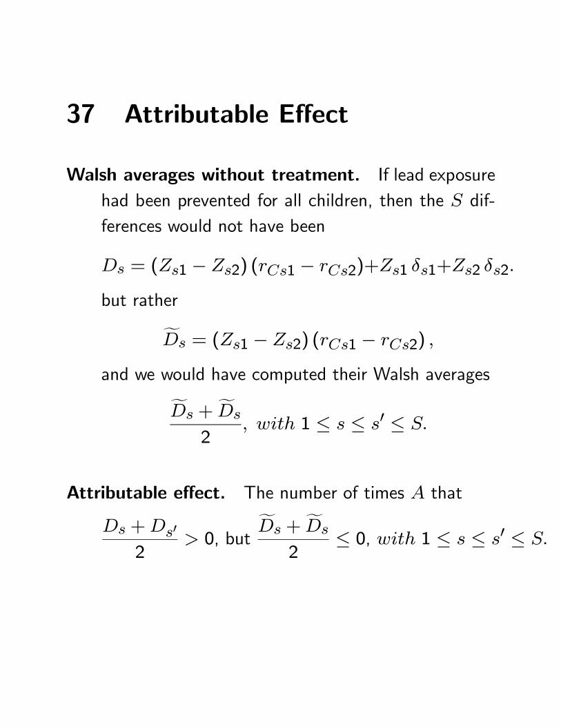
37 Attributable Effect

Walsh averages without treatment. If lead exposurehad been prevented for all children, then the S dif-ferences would not have been

Ds = (Zs1 − Zs2) (rCs1 − rCs2)+Zs1 δs1+Zs2 δs2.

but rather

fDs = (Zs1 − Zs2) (rCs1 − rCs2) ,

and we would have computed their Walsh averages

fDs + fDs

2, with 1 ≤ s ≤ s0 ≤ S.

Attributable effect. The number of times A that

Ds +Ds02

> 0, butfDs + fDs

2≤ 0, with 1 ≤ s ≤ s0 ≤ S.

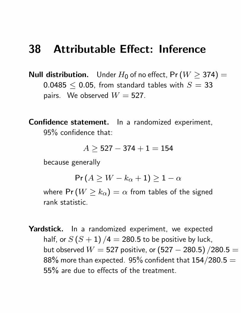
38 Attributable Effect: Inference

Null distribution. UnderH0 of no effect, Pr (W ≥ 374) =0.0485 ≤ 0.05, from standard tables with S = 33

pairs. We observed W = 527.

Confidence statement. In a randomized experiment,95% confidence that:

A ≥ 527− 374 + 1 = 154because generally

Pr (A ≥W − kα + 1) ≥ 1− α

where Pr (W ≥ kα) = α from tables of the signedrank statistic.

Yardstick. In a randomized experiment, we expectedhalf, or S (S + 1) /4 = 280.5 to be positive by luck,but observedW = 527 positive, or (527− 280.5) /280.5 =88%more than expected. 95% confident that 154/280.5 =55% are due to effects of the treatment.

39 But the study was not random-

ized . . .

Not randomized. The analysis would have been justi-fied by randomization in a randomized experiment.

Unknown assignment probabilities. An observationalstudy is a study of treatment effects in which eachperson has an unknown probability of treatment, typ-ically different probabilities for different people.

Simple model. In some finite population of people, j =1, . . . , J , person j has probability πj = Pr

³Zj = 1

´of exposure to treatment, where πj is not known.Probabilities are always conditional on things we re-gard as fixed, usually measured and unmeasured co-variates, potential outcomes,

³rTj, rCj

´, etc.

40 Simple model continued . . .

Covariates. The people, j = 1, . . . , J , in the finitepopulation have observed covariates xj and unob-served covariate uj. In the example, xj describeschild’s age and neighborhood.

Absolutely simplest case: Select S pairs, i = 1, 2,one treated, one control, from the J people in thepopulation. Match exactly for x, so that xs1 = xs2for each s, s = 1, . . . , S.

Matching algorithm: In this simplest case, the match-ing algorithm is permitted to use only x and 1 =Zs1 + Zs2.

41 Minor Issue: Dependence Among

Assignments

Experiments. In most experiments, treatment assign-ments are dependent in simple says; eg, half the peo-ple get treatment. Or one person in each pair getstreatment. Shapes randomization distributions.

Goal: Keep the model for observational studies parallelto experiments, but keep it simple.

Solution: Dependence introduced by conditioning.Nice way to handle this is to make the Zj indepen-dent and then introduce dependence by conditioning,eg on 1 = Zs1 + Zs2.

42 Is the randomization analysis ever

appropriate?

Ignorability, etc. Cluster of concepts – ignorability,strong ignorability, free of hidden bias, no unmea-sured confounders, etc. – .with similar intuition.

Intuition: Answers the theoretical question: When isit enough to adjust for the observed covariates youhave, xj?

A theoretical question. Frames the discussion, but doesn’ttell you what to make of data. In observationalstudies you always: (i) adjust for the covariates youhave xj, (ii) worry that you omitted some important(unobserved covariate) uj, and try to find ways toaddress this possibility.

43 Free of hidden bias

Definition. Treatment assignment is free of hidden biasif πj is a (typically unknown) function of xj – twopeople with the same xj have the same πj.

Intuition. A kid j who lives 30 miles from the batteryfactory is less likely to have a dad working in factorythan a kid k who lives two miles from the factory,πj < πk, but two kids of the same age who nextdoor are equally likely to have a dad in the factory.

But they didn’t match on kid’s gender. If gender werenot recorded, it would violate ‘free of hidden bias’ if(roughly) boys were more likely (or less likely) thangirls to have a dad working in the battery factor.

44 If free of hidden bias . . .

Problem: Unlike an experiment, πj are unknown.

If free of hidden bias: Two people with the same xjhave the same πj, which is typically unknown.

Eliminate unknowns by conditioning: If we match ex-actly for x, so xs1 = xs2, then

Pr (Zs1 = 1 | Zs1 + Zs2)

=πs1 (1− πs2)

πs1 (1− πs2) + πs2 (1− πs1)=1

2

because πs1 = πs2. A little more work shows thatwe get the randomization distribution by condition-ing.

More generally, This argument is quite general, work-ing for matched sets, strata, and more complex prob-lems.

45 Interpretation

If free of hidden bias: Two people with the same xjhave the same πj, which is typically unknown.

When do adjustments work? If a study is free of hid-den bias, if the only bias is due to observed covari-ates xj, even if the bias is unknown, the bias canbe removed in various ways, such as matching onxj, and conventional randomization inferences yieldappropriate inferences about treatment effect.

Key, if problematic, assumption. Identifies the keyassumption, but of course, doesn’t make it true. Fo-cuses attention, frames discussion. In contrast, inan experiment, randomization makes it true.

Divides methods. Methods of adjustment for x shouldwork when study is free of hidden bias. Need othermethods to address concerns about whether the studyis free of hidden bias.

46 Propensity Scores

Many observed covariates. If x is of high dimension,it’s hard to match. With just 20 binary covariates,there are 220 or about a million covariate patterns.

If free of hidden bias: Two people with the same xjhave the same πj, so πj is a function of xj, sayπj = e

³xj´, which is then called the propensity

score. .

Old argument again: Match exactly for x, so xs1 =xs2, then

Pr (Zs1 = 1 | Zs1 + Zs2)

=πs1 (1− πs2)

πs1 (1− πs2) + πs2 (1− πs1)=1

2

because πs1 = πs2 or e (xs1) = e (xs2)

Key point: Don’t need to match on high dimension x,just need to match on the scalar e (x).

47 Balancing with Propensity Scores

Whether or not the study is free of hidden bias, match-ing on propensity scores e = e (x) tends to balancethe observed covariates x used in the score. Definee = e (x) = Pr (Z = 1 |x), so the study is free ofhidden bias if πj = e

³xj´for all j, but e (x) is

defined even if πj depends on things besides x.

That is:

Pr (x |Z = 1, e) = Pr (x |Z = 0, e)

or x | | Z | e (x)

Proof: Suffices to show Pr Z = 1 |x, e (x) equalsPr Z = 1 | e (x). But Pr Z = 1 |x, e (x)= Pr (Z = 1 |x)which is just e (x). Also, Pr Z = 1 | e (x) equalsE [Pr Z = 1 |x, e (x) | e (x)]=E [Pr Z = 1 |x | e (x)]= E [e (x) | e (x)] = e (x).

48 Propensity Scores: Example

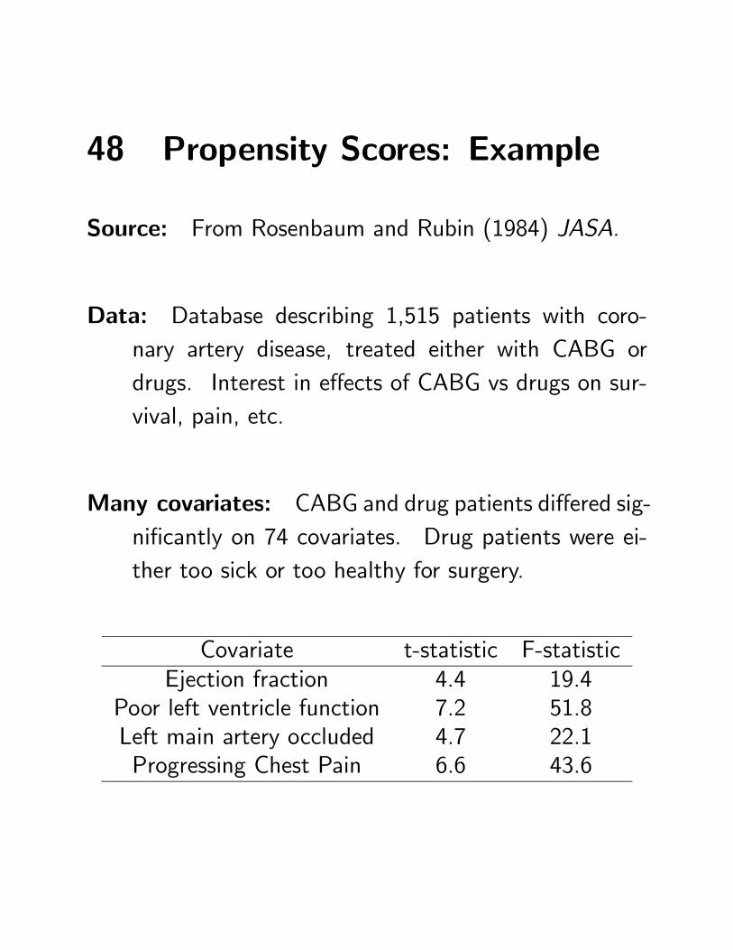
Source: From Rosenbaum and Rubin (1984) JASA.

Data: Database describing 1,515 patients with coro-nary artery disease, treated either with CABG ordrugs. Interest in effects of CABG vs drugs on sur-vival, pain, etc.

Many covariates: CABG and drug patients differed sig-nificantly on 74 covariates. Drug patients were ei-ther too sick or too healthy for surgery.

Covariate t-statistic F-statisticEjection fraction 4.4 19.4

Poor left ventricle function 7.2 51.8Left main artery occluded 4.7 22.1Progressing Chest Pain 6.6 43.6

1020

3040

50

Before Stratification

F-S

tatis

tic fo

r Cov

aria

te B

alan

ce

Figure 3:

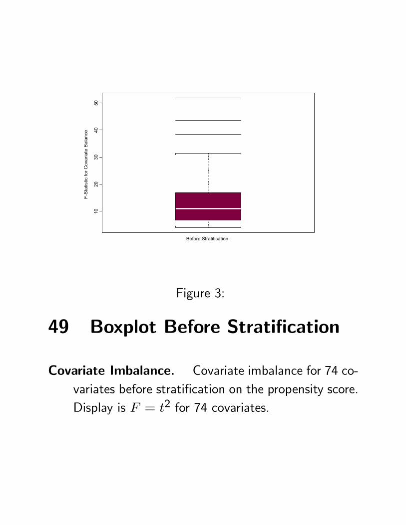
49 Boxplot Before Stratification

Covariate Imbalance. Covariate imbalance for 74 co-variates before stratification on the propensity score.Display is F = t2 for 74 covariates.

50 Procedure

Propensity score: Estimated using logit regression oftreatment (CABG or drugs) on covariates, some quadrat-ics, some interactions.

Five strata: Five groups formed at quintiles of the es-timated propensity score.

Counts of Patients in Strata

Propensity Score Stratum Medical Surgical1 = lowest = mostmedical 277 26

2 235 683 205 984 139 164

5 = highest = most surgical 69 234

51 Checking balance

2-Way 5× 2 Anova for Each Covariate

Propensity Score Stratum Medical Surgical1 = lowest = mostmedical

234

5 = highest = most surgical

Balance check. Main effect and interaction F−statistics.

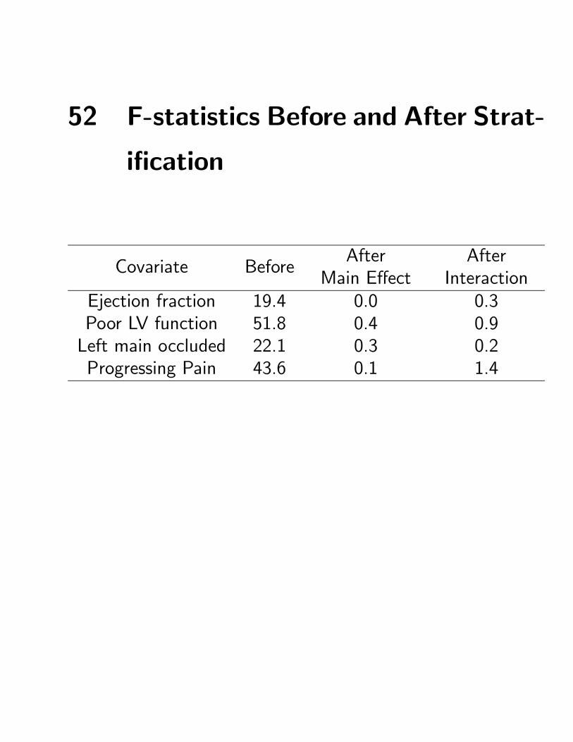
52 F-statistics Before and After Strat-

ification

Covariate BeforeAfter

Main EffectAfter

InteractionEjection fraction 19.4 0.0 0.3Poor LV function 51.8 0.4 0.9Left main occluded 22.1 0.3 0.2Progressing Pain 43.6 0.1 1.4

010

2030

4050

Before After/Main Ef After/Interaction

F-S

tatis

tic fo

r Cov

aria

te B

alan

ce

Figure 4:

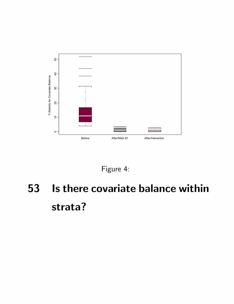
53 Is there covariate balance within

strata?

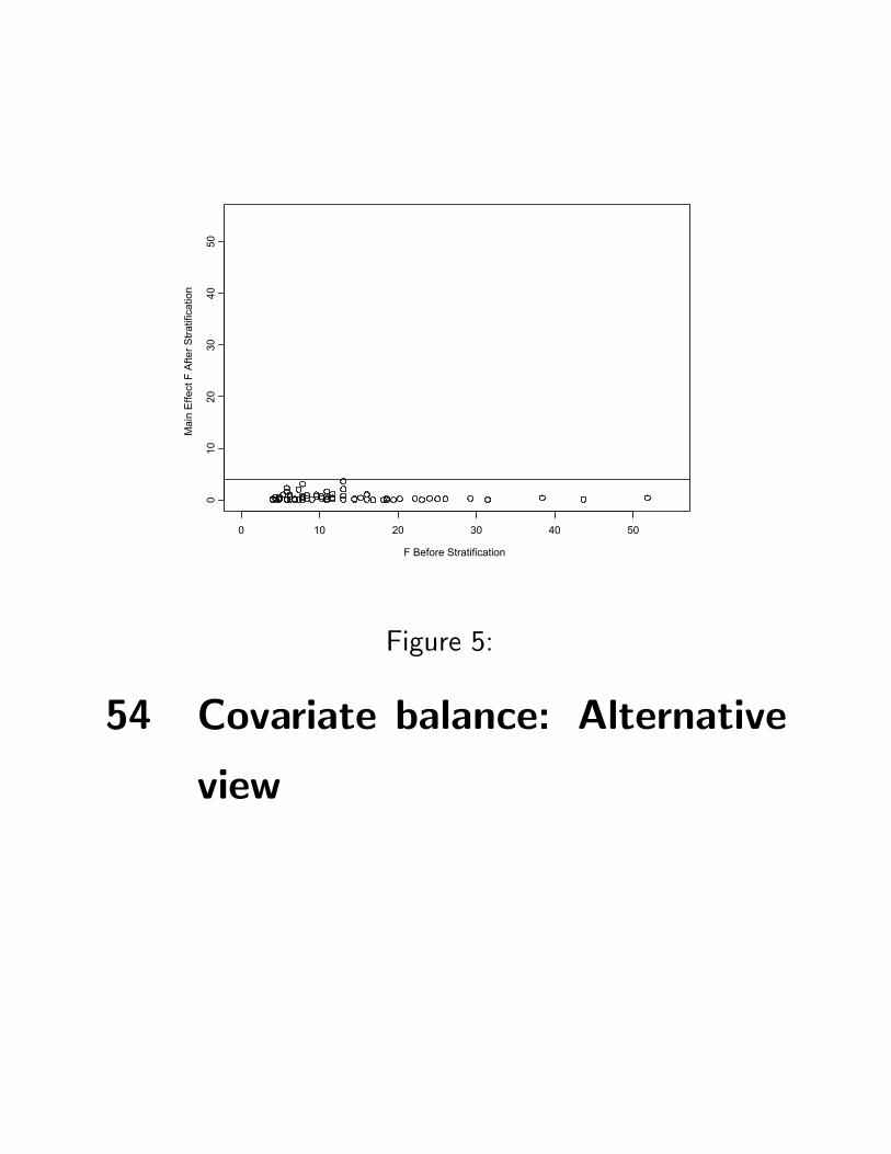
F Before Stratification

Mai

n E

ffect

F A

fter S

tratif

icat

ion

0 10 20 30 40 50

010

2030

4050

Figure 5:

54 Covariate balance: Alternative

view

55 Last words about propensity scores

Balancing. Stratifying or matching on a scalar propen-sity score tends to balance many observed covariates.

Effects of estimating the score. Examples, simulations,limited theory suggest estimated scores provide slightlymore than true propensity scores.

Other methods. Various methods permit explicit ac-knowledgement of use of estimated scores.

Key limitation. Propensity scores balance only observedcovariates, whereas randomization also balances un-observed covariates.

56 Addressing hidden bias

If free of hidden bias: Two people with the same ob-served xj have the same πj, which is typically un-known. Can remove the overt biases due to xj.

Common objection: Critic says: “Adjusting for xj isnot sufficient, because there is an unobserved uj,and adjustments for

³xj, uj

´were needed.”

That is, the objection asserts that, or raises the possi-bility that, the observed association between treat-ment Zj and response Rj is not an effect caused bythe treatment, but rather due to hidden bias fromtheir shared relationship with uj.

Formally, treatment assignment Zj and response Rj =rCj + Zj

³rTj − rCj

´may be associated because

rTj−rCj 6= 0 (a treatment effect) or because rTj−rCj = 0 but πj and rCj both vary with uj (a hiddenbias due to uj).

57 Sensitivity analysis

Question answered by a sensitivity analysis: If theobjection were true, if the association between treat-ment Zj and response Rj were due to hidden biasfrom uj, then what would uj have to be like?

What does the counter-claim actually claim? A sen-sitivity analysis looks at the observed data and usesit to clarify what the critic’s counter claim is actuallyclaiming.

Sensitivity varies. Studies vary markedly in how sen-sitive they are to hidden bias.

58 First Sensitivity Analysis

Cornfield, et al. (1959): they write:

“If an agent, A, with no causal effect upon the risk ofa disease, nevertheless, because of a positive correlationwith some other causal agent, B, shows an apparent risk,r, for those exposed to A, relative to those not so ex-posed, then the prevalence of B, among those exposed toA, relative to the prevalence among those not so exposed,must be greater than r.

Thus, if cigarette smokers have 9 times the risk of non-smokers for developing lung cancer, and this is not be-cause cigarette smoke is a causal agent, but only becausecigarette smokers produce hormone X, then the propor-tion of hormone X-producers among cigarette smokersmust be at least 9 times greater than that of nonsmok-ers. If the relative prevalence of hormone X-producers isconsiderably less than ninefold, then hormone X cannotaccount for the magnitude of the apparent effect.”

59 The Cornfield, et al Inequality

The Cornfield, et al sensitivity analysis is an importantconceptual advance:

“Association does not imply causation

– hidden bias can produce associations,”

is replaced by

“To explain away the association actually seen,

hidden biases would have to be of such and

such a magnitude.”

Provides a quantitative measure of uncertainty in lightof data.

As a confidence interval measures sampling uncertaintywithout making it go away, a sensitivity analysis mea-sure uncertainty due to hidden bias without makingthe uncertainty go away.

60 Alternative sensitivity analysis

Limitations. Cornfield’s inequality concerns binary re-sponses only and ignores sampling variability. Notexplicit about observed covariates.

Alternative formulation. Two subjects, j and k, withthe same observed covariates, xj = xk, may differin terms of uj and uk so that their odds of exposureto treatment differ by a factor of Γ ≥ 1,

1

Γ≤ πj (1− πk)

πk³1− πj

´ ≤ Γ.

Free of hidden bias is then Γ = 1.

When bias is present, when Γ > 1, the unknown πjcannot be eliminated, as before, by matching on xj,so the randomization distribution is no longer justi-fied.

61 Alternative sensitivity analysis,continued

Model. Two subjects, j and k, with xj = xk, maydiffer their odds of exposure to treatment differ by afactor of Γ ≥ 1,

1

Γ≤ πj (1− πk)

πk³1− πj

´ ≤ Γ (1)

so Γ provides measured departure from “no hiddenbias.”

Intuition: If Γ = 1.001, the πj are unknown, but al-most the same. If Γ = 5, πj are unknown and couldbe very different.

Plan. For each Γ ≥ 1, find upper and lower boundson inference quantities, like P-values (or endpoints ofconfidence intervals), for πj’s satisfying (1). Reportthese for several Γ. When do conclusions begin tochange?

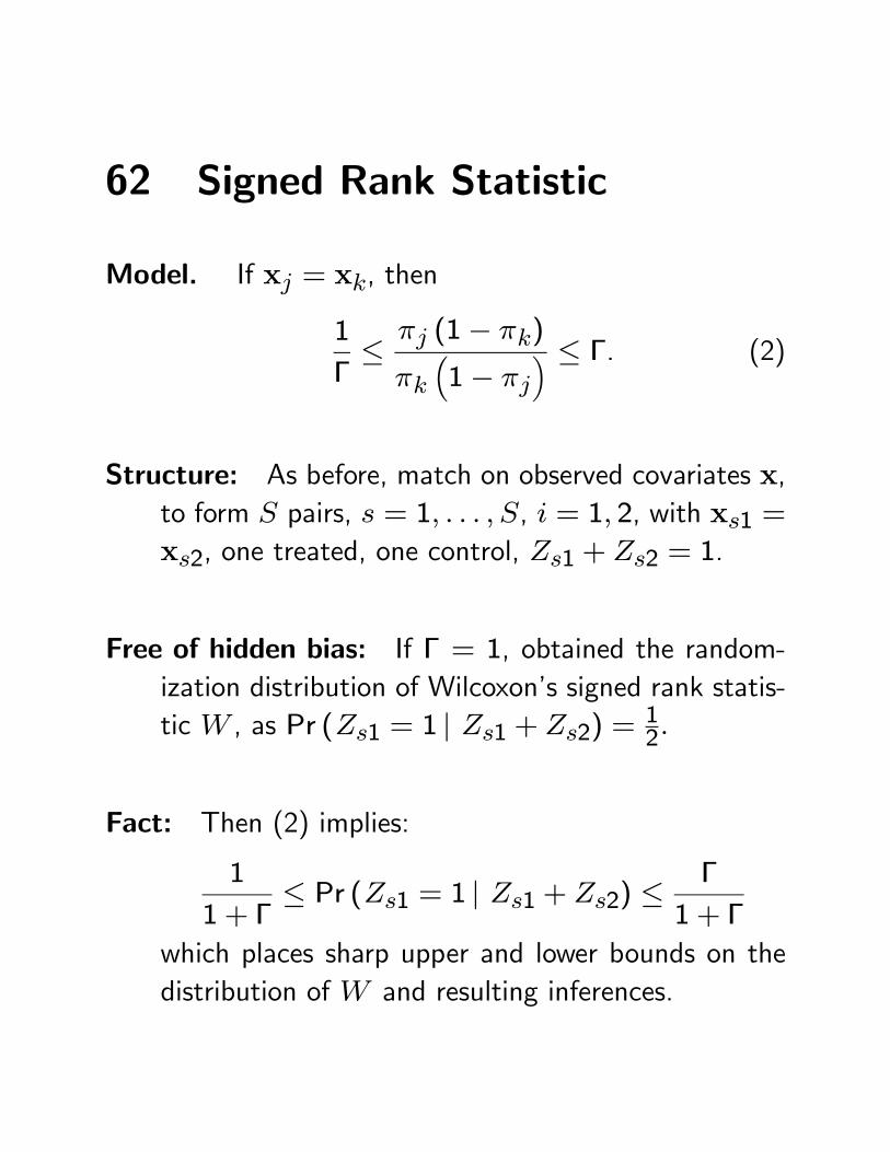
62 Signed Rank Statistic

Model. If xj = xk, then

1

Γ≤ πj (1− πk)

πk³1− πj

´ ≤ Γ. (2)

Structure: As before, match on observed covariates x,to form S pairs, s = 1, . . . , S, i = 1, 2, with xs1 =xs2, one treated, one control, Zs1 + Zs2 = 1.

Free of hidden bias: If Γ = 1, obtained the random-ization distribution of Wilcoxon’s signed rank statis-tic W , as Pr (Zs1 = 1 | Zs1 + Zs2) =

12.

Fact: Then (2) implies:

1

1 + Γ≤ Pr (Zs1 = 1 | Zs1 + Zs2) ≤

Γ

1 + Γ

which places sharp upper and lower bounds on thedistribution of W and resulting inferences.

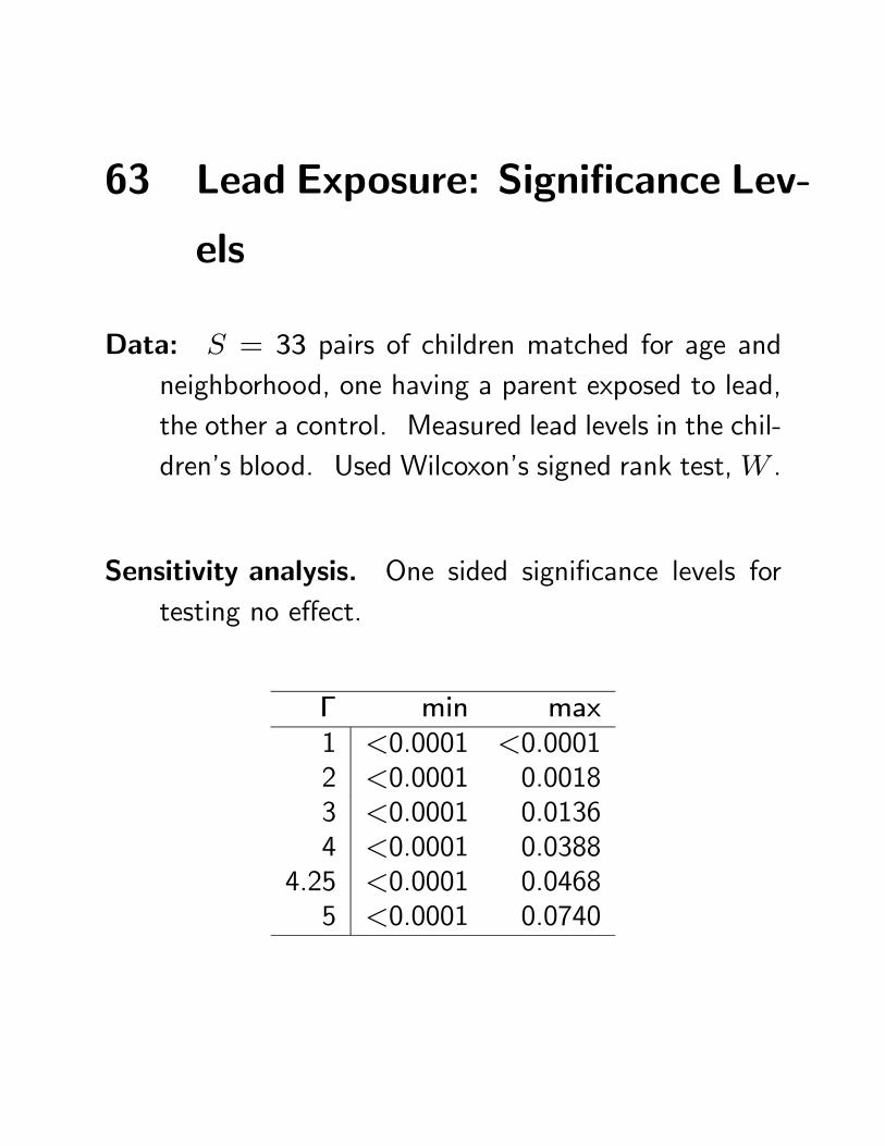
63 Lead Exposure: Significance Lev-

els

Data: S = 33 pairs of children matched for age andneighborhood, one having a parent exposed to lead,the other a control. Measured lead levels in the chil-dren’s blood. Used Wilcoxon’s signed rank test,W .

Sensitivity analysis. One sided significance levels fortesting no effect.

Γ min max1 <0.0001 <0.00012 <0.0001 0.00183 <0.0001 0.01364 <0.0001 0.0388

4.25 <0.0001 0.04685 <0.0001 0.0740

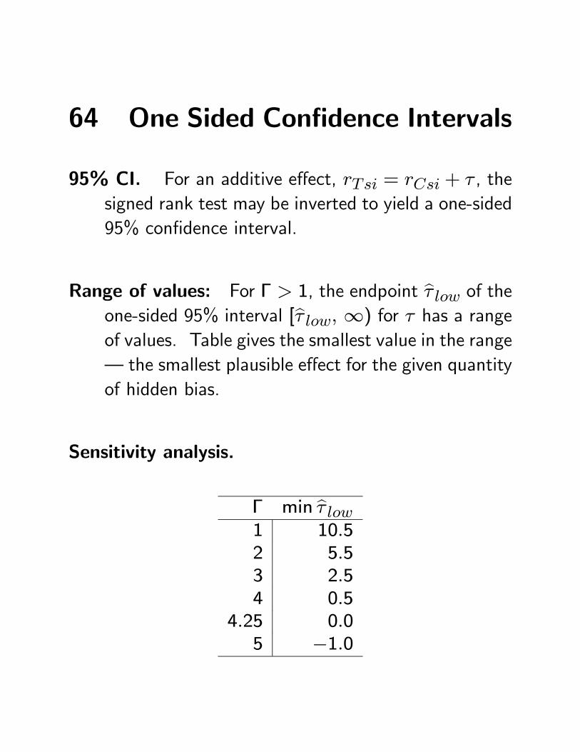
64 One Sided Confidence Intervals

95% CI. For an additive effect, rTsi = rCsi + τ , thesigned rank test may be inverted to yield a one-sided95% confidence interval.

Range of values: For Γ > 1, the endpoint bτ low of theone-sided 95% interval [bτ low, ∞) for τ has a rangeof values. Table gives the smallest value in the range– the smallest plausible effect for the given quantityof hidden bias.

Sensitivity analysis.

Γ min bτ low1 10.52 5.53 2.54 0.5

4.25 0.05 −1.0

65 Comparing Different Studies

Studies vary markedly in their sensitivity to hidden bias.

Treatment Γ = 1 (Γ, maxP − value)Smoking/Lung CancerHammond 1964

<0.0001 (5, 0.03)

DES/vaginal cancerHerbst, et al. 1976

< 0.0001 (7, 0.054)

Lead/Blood leadMorton, et al.1982

< 0.0001 (4.25, 0.047)

Coffee/MIJick, et al. 1973

0.0038 (1.3, 0.056)

Small biases could explain Coffee/MI association. Verylarge biases would be needed to explain DES/vaginalcancer association.

66 Sensitivity Analysis: Interpreta-

tion

Uses data, says something tangible. Replaces qual-itative “association does not imply causation,” by aquantitative statement based on observed data, “toexplain away observed associations as noncausal, hid-den biases would have to be of such and such a mag-nitude.”

Measures uncertainty. Measures uncertainty due tohidden bias, but does not dispel it. (As a confidenceinterval measures sampling uncertainty but does notdispel it.)

Fact of the matter. Your opinion about how much hid-den bias is present is your opinion. But the degreeof sensitivity to hidden bias is a fact of the matter,something visible in observed data.

67 Hill on Causality

Who was Hill? With Sir Richard Doll, Sir Austin Brad-ford Hill did some of the most careful and influentialstudies of smoking and health.

Hill’s Aspects: In 1965, Hill wrote a paper “The envi-ronment and disease: association or causation.” Heasked:

“Our observations reveal an association be-tween two variables, perfectly clear-cut and be-yond what we would care to attribute to theplay of chance. What aspects of that associa-tion should we especially consider before decid-ing that the mostly likely interpretation of it iscausation?”

i.e., after adjusting for biases we can see, what as-pects of the observed association provide informationabout cause and effect vs hidden bias?

68 Hill on Causality, continued.

Nine aspects: Strength, consistency, specificity, tem-porality, biological gradient, plausibility, coherence,experiment, analogy.

Consistency: “Has [the association] been repeatedlyobserved by different persons, in different places, cir-cumstances and times?”

Biological gradient: “[I]f the association is one whichcan reveal a biological gradient, or dose-responsecurve, the we should look most carefully for suchevidence.”

Coherence: “[T]he cause-and-effect interpretation . . .should not seriously conflict with generally knownfacts of the natural history and biology of the dis-ease.”

69 Reactions to Hill’s Aspects

Influence: Discussed in many textbooks in epidemiol-ogy, often mentioned in empirical papers.

Critics: Rothman, Sartwell, others have been critical ofHill’s aspects, perhaps not so much in the form Hilldescribed them, but rather in the more rigid way theyare sometimes described in textbooks.

Was Hill correct? As Hill often adjusted for observedcovariates, it is clear that his aspects are intended toprovide information about hidden bias. Do they?

70 Pattern matching

Social sciences: Similar considerations are referred toas “pattern matching.”

Cook and Shadish 1994, p. 565: ‘Successful predic-tion of a complex pattern of multivariate results of-ten leaves few plausible alternative explanations.’

Trochim 1985, p. 580: ‘. . . with more pattern speci-ficity it is generally less likely that plausible alterna-tive explanations for the observed effect pattern willbe forthcoming.’

Campbell 1988, p. 33: ‘. . . great inferential strengthis added when each theoretical parameter is exem-plified in two or more ways, each mode being asindependent as possible of the other, as far as thetheoretically irrelevant components are concerned’

71 More on pattern matching

Cook, Campbell, Peracchio (1990): “. . . the warrantfor causal inferences from quasi-experiments rests[on] structural elements of design other than ran-dom assignment — pretests, comparison groups, theway treatments are scheduled across groups . . . –[which] provide the best way of ruling out threats tointernal validity . . . [C]onclusions are more plausibleif they are based on evidence that corroborates nu-merous, complex, or numerically precise predictionsdrawn from a descriptive causal hypothesis.”

72 Fisher’s Comment: Elaborate The-

ories

Cochran (1965, §5): “About 20 years ago, when askedin a meeting what can be done in observational stud-ies to clarify the step from association to causation,Sir Ronald Fisher replied: ‘Make your theories elab-orate.’ The reply puzzled me at first, since by Oc-cam’s razor, the advice usually given is to make theo-ries as simple as is consistent with known data. WhatSir Ronald meant, as subsequent discussion showed,was that when constructing a causal hypothesis oneshould envisage as many different consequences ofits truth as possible, and plan observational studiesto discover whether each of these consequences isfound to hold.

. . . this multi-phasic attack is one of the mostpotent weapons in observational studies.”

73 Lead Example

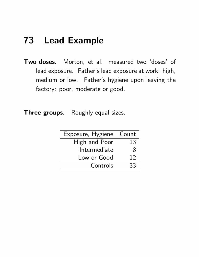
Two doses. Morton, et al. measured two ‘doses’ oflead exposure. Father’s lead exposure at work: high,medium or low. Father’s hygiene upon leaving thefactory: poor, moderate or good.

Three groups. Roughly equal sizes.

Exposure, Hygiene CountHigh and Poor 13Intermediate 8Low or Good 12

Controls 33

2040

60

High and Poor Intermediate Low or Good Controls

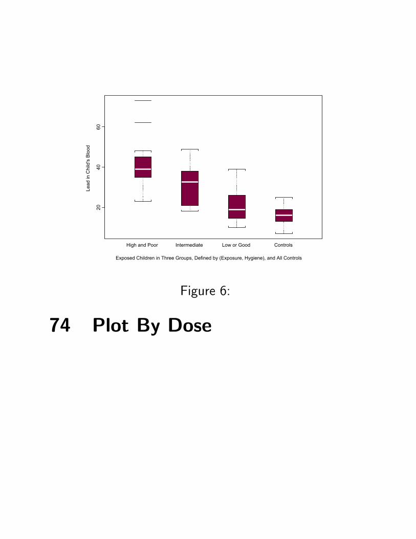
Exposed Children in Three Groups, Defined by (Exposure, Hygiene), and All Controls

Lead

in C

hild

's B

lood

Figure 6:

74 Plot By Dose

75 Coherent signed rank statistic

Pattern weighted. Matched pairs are weighted to re-flect anticipated pattern. May use doses (as here)or multivariate patterns, or both.

Here: (low exposure or good hygiene) pairs get weight1, (high exposure, poor hygiene) pairs get weight 2,intermediate pairs get 1.5.

Statistic: Sum of weight× rank (|Ds|) if Ds > 0.

Properties: If anticipated pattern is correct, greaterpower than W . If pattern is contradicted, typicallylower power.

76 Pattern Specificity and Sensi-

tivity to Hidden Bias

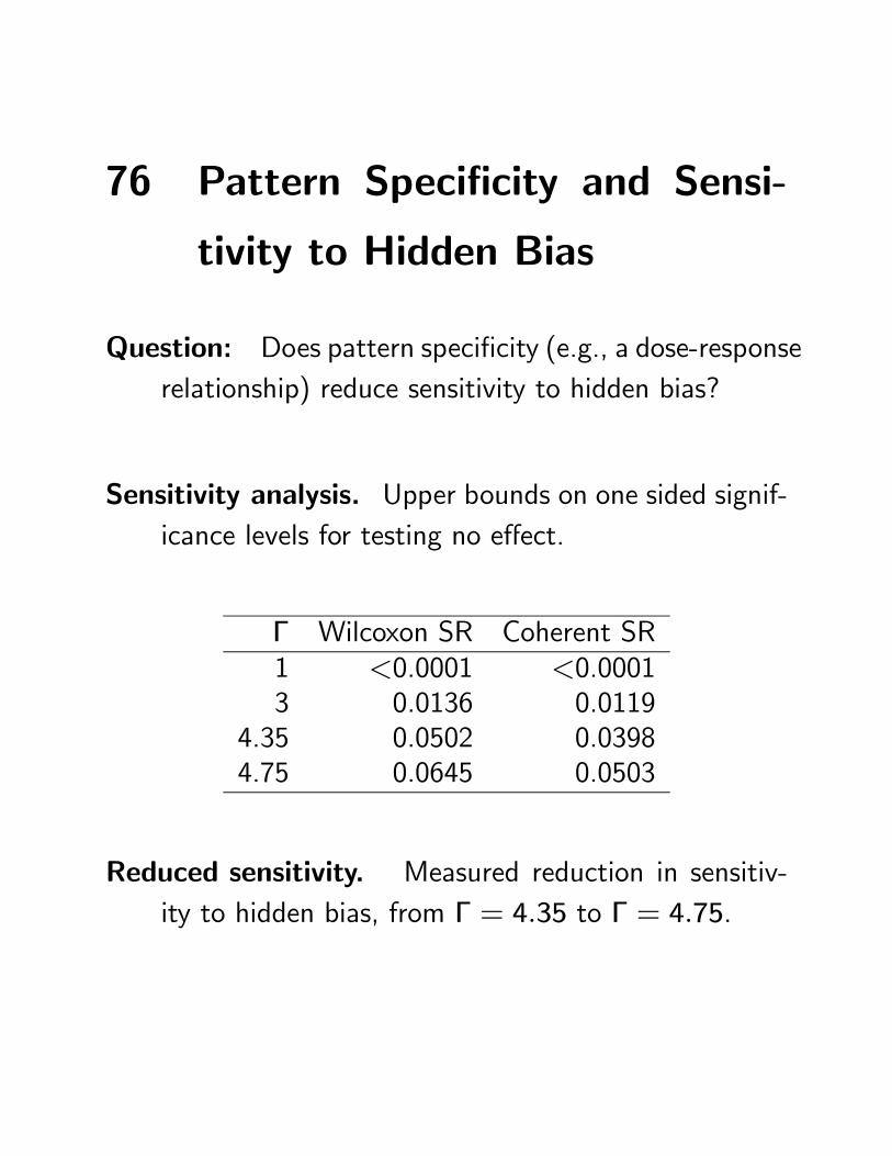
Question: Does pattern specificity (e.g., a dose-responserelationship) reduce sensitivity to hidden bias?

Sensitivity analysis. Upper bounds on one sided signif-icance levels for testing no effect.

Γ Wilcoxon SR Coherent SR1 <0.0001 <0.00013 0.0136 0.0119

4.35 0.0502 0.03984.75 0.0645 0.0503

Reduced sensitivity. Measured reduction in sensitiv-ity to hidden bias, from Γ = 4.35 to Γ = 4.75.

77 Reduced Sensitivity by Design

Can measure gain in term of Γ. Gains can be largeror small than in example, or no gain.

Design strategies. Moreover, can study theoretical sit-uations. Try to gain understand whether and whenstrategies reduce sensitivity to hidden bias.

Could look at ‘power’. Power of a sensitivity analysisfor specified Γ is the probability of an upper boundon the significance level of 0.05 or less.

Feasible but untidy. Power calculations of this sort de-pend on many things. Nicer to have somethinganalogous to Pitman efficiency.

78 Design Sensitivity

Relative performance in large samples. Limiting valueof Γ as sample size increases for competing strate-gies.

3 doses vs no doses. We used information on 3 doselevels vs ignoring doses in one data set.

With theory, We could make definitive comparisons ofvarious strategies under various conditions.

79 Some Strategies

Dose response. Hill’s suggestion: look for a dose-responserelationship.

Coherence among multiple outcomes. Campbell’s sug-gestion of multiple operationalism.

Clinical trials idea: Just two treatments that are asdifferent as possible. (Peto, et al. 1976)

80 Simple setting

Structure. S matched sets, match one treated to k

controls, k + 1 in each set.

Distribution. p-dimensional multivariate Normal responses,with errors that have constant intercorrelation ρ.(Campbell’s multiple operationalism)

Treatment effects. Proportional to dose, multiplierβ. (Hill’s dose-response)

Statistics. Stratified Wilcoxon rank sum statistic ap-plied to weighted combination of responses (Dawsonand Lagaokos 1993). Same weighted by doses.

81 Doses

Three patterns.µ1

2, 1,

3

2

¶produces a dose response

(1, 1, 1) same average dose, no dose response

µ3

2,3

2,3

2

¶different as possible, no dose response

Effect size. In computations shown here, effect at dose1 is half a standard deviation.

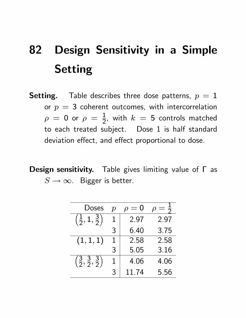
82 Design Sensitivity in a Simple

Setting

Setting. Table describes three dose patterns, p = 1

or p = 3 coherent outcomes, with intercorrelationρ = 0 or ρ = 1

2, with k = 5 controls matchedto each treated subject. Dose 1 is half standarddeviation effect, and effect proportional to dose.

Design sensitivity. Table gives limiting value of Γ asS →∞. Bigger is better.

Doses p ρ = 0 ρ = 12³

12, 1,

32

´1 2.97 2.973 6.40 3.75

(1, 1, 1) 1 2.58 2.583 5.05 3.16³

32,32,32

´1 4.06 4.063 11.74 5.56

83 Observations

Summary: Strategies can strongly affect sensitivity tohidden bias.

Specifics: Larger doses does most, then coherence amongoutcomes when error correlations are low, then doseresponse.

Traditional qualitative advice: Seems correct so faras it goes, but the relative (i.e. quantitative) im-portance and effectiveness of different strategies isonly beginning to be understood.

84 Summary

Causal effects. Comparison of potential outcomes un-der competing treatments – not jointly observable(Neyman 1923, Rubin 1974). .

Randomized experiments. Permit inference about theeffects caused by treatments (Fisher 1935).

Observational studies: Adjustments. Without ran-domization, adjustments are required. Straightfor-ward for observed covariates, but there might be im-portant covariates that you did not observe.

Observational studies: Sensitivity analysis. What wouldunobserved covariates have to be like to alter con-clusions? (Cornfield, et al.)

Observational studies: Pattern specificity. Reducingsensitivity to hidden bias. (Campbell 1988, Hill 1965)