Copyright by Amogh V. Prabhu 2008

Copyright

by

Amogh V. Prabhu

2008

The Dissertation Committee for Amogh V. Prabhucertifies that this is the approved version of the following dissertation:

Performance Monitoring of Run-to-Run Control

Systems Used in Semiconductor Manufacturing

Committee:

Thomas F. Edgar, Supervisor

S. Joe Qin

Venkat Ganesan

Glenn Y. Masada

Maruthi R. Akella

Michael L. Miller



by

Amogh V. Prabhu, B. Chem. Engg.

DISSERTATION

Presented to the Faculty of the Graduate School of

The University of Texas at Austin

in Partial Fulfillment

of the Requirements

for the Degree of

DOCTOR OF PHILOSOPHY

THE UNIVERSITY OF TEXAS AT AUSTIN

August 2008

Dedicated to my parents.

Acknowledgments

First of all, I wish to thank Dr. Edgar for providing me an opportunity

to pursue my PhD degree at the University of Texas. He has been very patient

with me and has kept me on track through the last four years.

I would also like to thank Dr. Qin, Dr. Ganesan, Dr. Masada, Dr. Akella

and Dr. Miller for serving as my committee members. In addition, I thank all

the professors at the University of Texas who enhanced my knowledge of the

process control area.

This dissertation would not have been possible without the support of

the Advanced Process Control group at Advanced Micro Devices (AMD) and

the initiative taken by Matt Purdy and Robert Chong. I thank Rob for having

faith in my abilities and supporting the work I did in the company. I must

thank Rick Good for jump-starting my thesis work when I needed it the most

and for being a good source for laughs during my time there.

I also thank Kevin Lensing, Mike ‘Big Mike’ Forsberg, Alok Vaid, Elfido

Coss, Broc Stirton, Siddharth Chauhan and Jin Wang for helping me out on

several occasions and helping me enjoy the time I spent at AMD.

My labmates from the Edgar group and Dr. Qin’s group have been a

great source of knowledge and distractions on various topics. I particularly

liked the multicultural mix in our group, with people from eight different

v

countries. I would especially thank Hyung, John Hedengren, Terry, Xiaoliang,

Clare, Dan Barad, Yang, Dan Weber, Sidharth Abrol, Carlos, Ivan, Kye-Hyun

Baek, Ben Spivey and Bhalinder Gill. I wish all of them good luck in their

future careers.

My stay in Austin over the last four years has been made enjoyable

by three wonderful roommates Gaurav Goel, Manas, and Gaurav Gupta. I

will treasure the memories of the innumerable movies we saw, the long-lasting

poker/monopoly games we played and the unending discussions we had on

any topic ranging from the inane to the intellectual. Along with these guys, I

also had a great time with Mehul, Landry, Karthik, Sachin and Raee, Vipin,

Harish and Jasraj. I will miss you all and I will miss living in Austin.

Lastly, I would like to thank my family for supporting me all these

years. Pappa and Aai, you have been a great source of inspiration for me. My

two sisters, Chiku and Mini, have been great company all these years and I

always wish they were with me wherever I go. I hope all their dreams for their

families come true.

vi



Publication No.

Amogh V. Prabhu, Ph.D.

The University of Texas at Austin, 2008

Supervisor: Thomas F. Edgar

Monitoring and diagnosis of the control system, though widely used

in the chemical processing industry, is currently lacking in the semiconductor

manufacturing industry. This work provides methods for performance assess-

ment of the most commonly used control system in this industry, namely,

run-to-run process control.

First, an iterative solution method for the calculation of best achievable

performance of the widely used run-to-run Exponentially Weighted Moving

Average (EWMA) controller is derived. A normalized performance index is

then defined based on the best achievable performance. The effect of model

mismatch in the process gain and disturbance model parameter, delays, bias

changes and nonlinearity in the process is then studied. The utility of the

method under manufacturing conditions is tested by analyzing three processes

from the semiconductor industry.

vii

Missing measurements due to delay are estimated using the disturbance

model for the process. A minimum norm estimation method coupled with

Tikhonov regularization is developed. Simulations are then carried out to

investigate disturbance model mismatch, gain mismatch and different sampling

rates. Next, the forward and backward Kalman filter are applied to obtain the

missing values and compared with previous examples. Manufacturing data

from three processes is then analyzed for different sampling rates.

Existing methods are compared with a new method for state estima-

tion in high-mix manufacturing. The new method is based on a random walk

model for the context states. This approach is also combined with the recur-

sive equations of the Kalman filter. The method is applied to an industrial

exposure process by extending the random walk model into an integrated mov-

ing average model and weights used to give preference to the context that is

more frequent.

Finally, a performance metric is derived for PID controllers, when they

are used to control nonlinear processes. Techniques to identify nonlinearity

in a process are introduced and polynomial NARX models are proposed to

represent a nonlinear process. A performance monitoring technique used for

MIMO processes is then applied. Finally, the method is applied to an EWMA

control case used before, a P/PI control case from literature and two cases

from the semiconductor industry.

viii

Table of Contents

Acknowledgments v

Abstract vii

List of Tables xv

List of Figures xvi

Chapter 1. Introduction 1

1.1 Semiconductor manufacturing . . . . . . . . . . . . . . . . . . 1

1.1.1 Lithography process . . . . . . . . . . . . . . . . . . . . 2

1.1.1.1 Exposure control . . . . . . . . . . . . . . . . . 3

1.1.1.2 Overlay Control . . . . . . . . . . . . . . . . . . 3

1.1.2 Etch process . . . . . . . . . . . . . . . . . . . . . . . . 4

1.1.2.1 STI etch . . . . . . . . . . . . . . . . . . . . . . 5

1.1.2.2 Gate etch . . . . . . . . . . . . . . . . . . . . . 5

1.1.2.3 BEOL etch . . . . . . . . . . . . . . . . . . . . 7

1.2 Process control in the semiconductor industry . . . . . . . . . 7

1.2.1 Run-to-Run process control . . . . . . . . . . . . . . . . 7

1.2.2 EWMA Controller . . . . . . . . . . . . . . . . . . . . . 9

1.2.3 Alternatives to EWMA-based run-to-run control . . . . 10

1.3 Threaded Control . . . . . . . . . . . . . . . . . . . . . . . . . 12

1.3.1 Non-threaded control . . . . . . . . . . . . . . . . . . . 13

1.4 Overview of dissertation . . . . . . . . . . . . . . . . . . . . . 14

1.4.1 EWMA controller optimization . . . . . . . . . . . . . . 15

1.4.2 Metrology delay compensation . . . . . . . . . . . . . . 16

1.4.3 Non-threaded controller state estimation . . . . . . . . . 17

1.4.4 Optimal parameters for nonlinear processes . . . . . . . 18

ix

Chapter 2. Performance Assessment of Run-to-RunEWMA Controllers 19

2.1 Introduction . . . . . . . . . . . . . . . . . . . . . . . . . . . . 19

2.1.1 Minimum variance control (MVC) . . . . . . . . . . . . 19

2.1.2 Alternative methods . . . . . . . . . . . . . . . . . . . . 20

2.1.3 Performance monitoring for semiconductor manufacturing 26

2.2 Theory Development . . . . . . . . . . . . . . . . . . . . . . . 28

2.2.1 Discrete integral controller . . . . . . . . . . . . . . . . 28

2.2.2 Optimal controller gain . . . . . . . . . . . . . . . . . . 30

2.2.3 EWMA Controller . . . . . . . . . . . . . . . . . . . . . 31

2.2.3.1 Equivalence to an internal model control (IMC)structure . . . . . . . . . . . . . . . . . . . . . . 32

2.2.3.2 Minimum mean squared error forecast . . . . . 33

2.2.4 Sources of model error . . . . . . . . . . . . . . . . . . . 33

2.3 Simulations . . . . . . . . . . . . . . . . . . . . . . . . . . . . 34

2.3.1 Data Analysis . . . . . . . . . . . . . . . . . . . . . . . 34

2.3.1.1 Moving Window . . . . . . . . . . . . . . . . . 35

2.3.1.2 Effect of moving window size . . . . . . . . . . 36

2.3.2 Model mismatch . . . . . . . . . . . . . . . . . . . . . . 36

2.3.2.1 Effect of gain mismatch . . . . . . . . . . . . . 38

2.3.2.2 Effect of error in disturbance parameter . . . . 39

2.3.3 Effect of delay . . . . . . . . . . . . . . . . . . . . . . . 41

2.3.3.1 Effect of process delays . . . . . . . . . . . . . . 41

2.3.3.2 Effect of metrology delays . . . . . . . . . . . . 44

2.3.4 Process changes . . . . . . . . . . . . . . . . . . . . . . 45

2.3.4.1 Effect of time-varying bias . . . . . . . . . . . . 46

2.3.4.2 Effect of step change in bias . . . . . . . . . . . 47

2.3.5 Nonlinear process . . . . . . . . . . . . . . . . . . . . . 48

2.4 Results from manufacturing data . . . . . . . . . . . . . . . . 51

2.4.1 Etch process A . . . . . . . . . . . . . . . . . . . . . . . 52

2.4.1.1 Distribution of performance indices . . . . . . . 52

2.4.1.2 Sample thread performance plots . . . . . . . . 53

2.4.2 Etch process B . . . . . . . . . . . . . . . . . . . . . . . 55

x



2.4.3 Exposure process . . . . . . . . . . . . . . . . . . . . . . 60



2.5 Conclusions and future work . . . . . . . . . . . . . . . . . . . 61

Chapter 3. Missing Data Estimation for Run-to-Run EWMA-controlled Processes 65

3.1 Introduction . . . . . . . . . . . . . . . . . . . . . . . . . . . . 65

3.1.1 Choice of estimation method . . . . . . . . . . . . . . . 66

3.1.2 Existing literature . . . . . . . . . . . . . . . . . . . . . 69

3.2 EWMA control . . . . . . . . . . . . . . . . . . . . . . . . . . 75

3.3 Minimum norm solution . . . . . . . . . . . . . . . . . . . . . 77

3.3.1 Simulations . . . . . . . . . . . . . . . . . . . . . . . . . 81

3.3.1.1 Example 1: RtR Simulated Data . . . . . . . . 81

3.3.1.2 Example 2: Comparison of alternative methods 81

3.3.1.3 Example 3: Effect of disturbance model mismatch 83

3.3.1.4 Example 4: Effect of sampling rate . . . . . . . 85

3.3.1.5 Example 5: Effect of gain mismatch . . . . . . . 85

3.4 Kalman filter solution . . . . . . . . . . . . . . . . . . . . . . . 87

3.4.1 State-space representation . . . . . . . . . . . . . . . . . 87

3.4.2 Kalman filter algorithm . . . . . . . . . . . . . . . . . . 88

3.4.2.1 Forward Kalman filter . . . . . . . . . . . . . . 89

3.4.2.2 Smoothed Kalman filter . . . . . . . . . . . . . 90

3.4.3 Using the minimum norm solution . . . . . . . . . . . . 91

3.4.4 Simulations . . . . . . . . . . . . . . . . . . . . . . . . . 92

3.4.4.1 Example 2 Revisited . . . . . . . . . . . . . . . 92





3.5.1 Etch process A . . . . . . . . . . . . . . . . . . . . . . . 96

xi

3.5.1.1 Effect of sampling rate . . . . . . . . . . . . . . 97

3.5.1.2 Cumulative study of all threads . . . . . . . . . 97

3.5.2 Etch process B . . . . . . . . . . . . . . . . . . . . . . . 99



3.5.3 Exposure process . . . . . . . . . . . . . . . . . . . . . . 101



3.5.4 Application to data reconstruction for controller perfor-mance monitoring . . . . . . . . . . . . . . . . . . . . . 105


Chapter 4. New State Estimation Methods for High-mix Semi-conductor Manufacturing Processes 110

4.1 Introduction . . . . . . . . . . . . . . . . . . . . . . . . . . . . 110

4.1.1 Run-to-run EWMA control . . . . . . . . . . . . . . . . 113

4.2 Previous methodologies . . . . . . . . . . . . . . . . . . . . . . 115

4.2.1 Threads . . . . . . . . . . . . . . . . . . . . . . . . . . . 116

4.2.2 Just-in-time adaptive disturbance estimation (JADE) . 118

4.2.3 Kalman filter-based approaches . . . . . . . . . . . . . . 120

4.2.4 Defining performance indices for estimation accuracy . . 122

4.3 New model-based algorithm . . . . . . . . . . . . . . . . . . . 122

4.3.1 Random walk model . . . . . . . . . . . . . . . . . . . . 123

4.3.2 Moving window approach . . . . . . . . . . . . . . . . . 126

4.3.3 Combination with Kalman filter . . . . . . . . . . . . . 127

4.4 Results from simulated data . . . . . . . . . . . . . . . . . . . 128

4.4.1 Effect of moving window size . . . . . . . . . . . . . . . 132

4.4.2 Effect of number of context items . . . . . . . . . . . . . 135


4.5.1 Model adjustment based on process knowledge . . . . . 138

4.5.2 Addition of context weights . . . . . . . . . . . . . . . . 140

4.5.3 Effect of moving window size . . . . . . . . . . . . . . . 142


xii

Chapter 5. Identification and Monitoring of PIDcontrolled Nonlinear Processes 146

5.1 Introduction . . . . . . . . . . . . . . . . . . . . . . . . . . . . 146

5.1.1 Types of nonlinear models . . . . . . . . . . . . . . . . . 147

5.1.2 Other methods dealing with nonlinear control . . . . . . 149

5.2 Detecting nonlinearity using higher order statistics . . . . . . . 151

5.2.1 Bispectrum and Bicoherence . . . . . . . . . . . . . . . 152

5.2.2 Nonlinearity and non-gaussianity . . . . . . . . . . . . . 154

5.2.2.1 Non-gaussianity test . . . . . . . . . . . . . . . 154

5.2.2.2 New nonlinearity test . . . . . . . . . . . . . . . 155

5.3 Polynomial NARX/NARMAX models . . . . . . . . . . . . . . 157

5.3.1 Least Squares solution . . . . . . . . . . . . . . . . . . . 159

5.3.2 Singular Value Decomposition . . . . . . . . . . . . . . 160

5.3.3 Orthogonal Least Squares . . . . . . . . . . . . . . . . . 160

5.3.4 Model order identification . . . . . . . . . . . . . . . . . 163

5.3.4.1 Lipschitz numbers . . . . . . . . . . . . . . . . 163

5.3.4.2 False nearest neighbors . . . . . . . . . . . . . . 164

5.3.5 Model Stability . . . . . . . . . . . . . . . . . . . . . . . 165

5.4 PID performance optimization . . . . . . . . . . . . . . . . . . 165

5.4.1 Theory development . . . . . . . . . . . . . . . . . . . . 166

5.4.2 Optimal PID parameters . . . . . . . . . . . . . . . . . 167

5.5 Results from nonlinear SISO models . . . . . . . . . . . . . . . 169

5.5.1 Example from Chapter 2 . . . . . . . . . . . . . . . . . 169

5.5.2 P/PI control of a Volterra model . . . . . . . . . . . . . 170

5.6 Results from nonlinear MISO models . . . . . . . . . . . . . . 174

5.6.1 Lithography dose-focus control . . . . . . . . . . . . . . 174

5.6.2 Back-end-of-line (BEOL) etch . . . . . . . . . . . . . . . 178


xiii

Chapter 6. Conclusions and Future Work 181

6.1 Key Results . . . . . . . . . . . . . . . . . . . . . . . . . . . . 181

6.1.1 Performance Assessment of Run-to-Run EWMAControllers . . . . . . . . . . . . . . . . . . . . . . . . . 181

6.1.2 Missing Data Estimation for Run-to-RunEWMA-controlled Processes . . . . . . . . . . . . . . . 182

6.1.3 New State Estimation Methods for High-mix Semicon-ductor Manufacturing Processes . . . . . . . . . . . . . 183

6.1.4 Identification and Monitoring of PID controlled Nonlin-ear Processes . . . . . . . . . . . . . . . . . . . . . . . . 184

6.2 Application in industry . . . . . . . . . . . . . . . . . . . . . . 185

6.3 Recommendations for future work . . . . . . . . . . . . . . . . 188

Appendices 192

Appendix A. EWMA and integral feedback control 193

Appendix B. EWMA control and IMA(1,1) model 195

Appendix C. Minimum norm solution 198

Appendix D. Tikhonov regularization 200

Appendix E. Proof of full rank context matrix 203

Bibliography 206

Vita 234

xiv

List of Tables

2.1 Effect of variable delay on performance index . . . . . . . . . . 45

3.1 Comparison with ad hoc techniques . . . . . . . . . . . . . . . 83

3.2 Comparison with previous techniques . . . . . . . . . . . . . . 92

4.1 Context probabilities . . . . . . . . . . . . . . . . . . . . . . . 130

xv

List of Figures

1.1 Steps in chip manufacturing . . . . . . . . . . . . . . . . . . . 2

1.2 Process flow for lithography . . . . . . . . . . . . . . . . . . . 4

1.3 STI etch profile . . . . . . . . . . . . . . . . . . . . . . . . . . 5

1.4 Gate etch profile . . . . . . . . . . . . . . . . . . . . . . . . . 6

2.1 IMC structure of an EWMA controller . . . . . . . . . . . . . 32

2.2 Variation in performance index with moving window size . . . 37

2.3 Effect of gain mismatch on performance index . . . . . . . . . 38

2.4 Effect of disturbance model mismatch on performance index . 40

2.5 Effect of integral delay on performance index . . . . . . . . . . 42

2.6 Effect of modeled delay on performance index . . . . . . . . . 43

2.7 Effect of drifting bias on performance index . . . . . . . . . . 47

2.8 Effect of step change in bias on performance index . . . . . . . 49

2.9 Effect of nonlinearity on performance index . . . . . . . . . . . 50

2.10 Distribution of performance indices for a nonlinear process . . 51

2.11 Distribution of performance indices for Etch A. . . . . . . . . 53

2.12 Change in performance index over time for Thread 1 in Etch A. 54





2.17 Distribution of performance indices for Etch B. . . . . . . . . 57

2.18 Change in performance index over time for Thread 1 in Etch B. 58



2.21 Distribution of performance indices for the exposure process. . 61

2.22 Change in performance index over time for Thread 1 in theexposure process. . . . . . . . . . . . . . . . . . . . . . . . . . 62

xvi

2.23 Change in performance index over time for Thread 2 in theexposure process. . . . . . . . . . . . . . . . . . . . . . . . . . 63

3.1 Simulation results for Example 1 . . . . . . . . . . . . . . . . 82

3.2 Change in MSE with change in mismatch for EWMA parameter 84

3.3 Change in MSE with change in sampling rate . . . . . . . . . 86

3.4 Change in MSE with gain mismatch . . . . . . . . . . . . . . . 87

3.5 Change in MSE with change in mismatch for EWMA parameter 93


3.7 Change in MSE with gain mismatch . . . . . . . . . . . . . . . 96


3.9 Cumulative study of etch process A . . . . . . . . . . . . . . . 99


3.11 Cumulative study of etch process B . . . . . . . . . . . . . . . 102


3.13 Cumulative study of exposure process . . . . . . . . . . . . . . 104

3.14 Improvement in performance with missing data estimation . . 106



4.1 Simulated data for Process 1 . . . . . . . . . . . . . . . . . . . 130



4.4 Effect of moving window size on mean squared error for process1. . . . . . . . . . . . . . . . . . . . . . . . . . . . . . . . . . . 133



4.7 Effect of increasing context items at constant window size onthe estimation performance index (EPI). . . . . . . . . . . . . 136

4.8 Number of threads with specified number of runs . . . . . . . 139

4.9 Effect of increasing weight on the machine context . . . . . . . 141

4.10 Effect of moving window size on the estimation error . . . . . 142

xvii

4.11 Change in error variance . . . . . . . . . . . . . . . . . . . . . 144

5.1 Squared bicoherence plot . . . . . . . . . . . . . . . . . . . . . 157

5.2 Response plot for EWMA example . . . . . . . . . . . . . . . 171

5.3 Response plot for proportional controller . . . . . . . . . . . . 172

5.4 Response plot for PI controller . . . . . . . . . . . . . . . . . . 173

5.5 Bossung curves of CD versus focus . . . . . . . . . . . . . . . 176

5.6 Response plot for lithography process . . . . . . . . . . . . . . 177

5.7 Response plot for BEOL etch process . . . . . . . . . . . . . . 179

6.1 Performance Monitoring Framework . . . . . . . . . . . . . . . 187

6.2 Nonlinear Performance Monitoring . . . . . . . . . . . . . . . 189

xviii

Chapter 1

Introduction

1.1 Semiconductor manufacturing

Silicon wafer manufacturing has seen rapid progress over the last 50

years due to vast improvements in production technology leading to ever

smaller dimensions within the chip at lower costs. The goal of the indus-

try as a whole is to continue this trend as the minimum feature size reduces

below 45 nm and the standard wafer dimension increases beyond 300 mm

over the next decade. This requires better control of the product yield and

throughput as well as less wastage because of qualification wafer usage and

wafer reworks. The major steps involved in a typical manufacturing facility

are shown in Figure (1.1).

Following is a description of the processes which are subject to run-

to-run process control in the semiconductor industry and are considered in

this work. Unless otherwise mentioned, the descriptions are from Doering and

Nishi [44].

1

Figure 1.1: Steps involved in a typical silicon manufacturing process. Thenumbered steps are 1. Wafer slicing 2. Wafer polishing 3. Chemical VaporDeposition 4. Photolithography 5. Etch 6. Repetition of steps (4) and (5)7. Doping 8. Chemical Mechanical Planarization and interconnects 9. Wafertesting and packaging. Source: www.sematech.org

1.1.1 Lithography process

A fundamental requirement for almost all useful semiconductor devices

is the definition of patterned elements. The overwhelming technology choice

for performing this patterning since the very inception of semiconductor man-

ufacturing has been optical lithography using ultraviolet (UV) light. It is the

most frequently used process in the chip fabrication facility (henceforth re-

ferred to as the fab), typically accounting for 30-35% of the total process cost.

Most commercial systems today use a step-and-scan approach for lithography.

Figure (1.2) shows the process flow for lithography [122].

Two of the most important parts of the lithography process with respect

to process control are feature delineation and the stacking of layers. These are

controlled by the exposure and overlay controllers respectively.

2

1.1.1.1 Exposure control

Accuracy in the critical dimension (CD) after lithography is required

at a number of steps such as shallow trench isolation etch, gate etch and

interconnect damascene patterning. This is reported to provide much tighter

control of the electrical properties of transistors. It is customary to consider

CD control of ±10% to be a requirement for a high-performance process. The

CD is known to be a function of the exposure dose and focus. The depth of

focus is generally flat in the given CD resolution. As a result, we can control

the CD by manipulating the exposure dose at every step. As image resolution

decreases, however, we may need to incorporate the focus as a variable. The

output of the lithography process is the CD and this can be measured using

either CD-SEM (scanning electron microscopy) or scatterometry.

1.1.1.2 Overlay Control

A fundamental requirement for semiconductor lithography is the place-

ment of all pattern edges in precisely the correct location with respect to ex-

isting patterns on the wafer, known as overlay. The most important sources of

overlay errors are mask errors, lens distortion and magnification, wafer distor-

tion, displacement of the wafer alignment keys, and overlay metrology errors.

The various errors can be driven to zero by either considering each separately

or by combining the errors into a linear model. Most overlay metrology is done

using an optical system that automatically evaluates how far from the center

the target pattern in the top layer is from the center of the target pattern in

3

the layer below.

Figure 1.2: Process flow for a lithography process. The exposure step usesdeep UV radiation passed through a reticle having the desired pattern.

1.1.2 Etch process

In integrated semiconductor manufacturing, plasma etching is usually

dealt with in the context of a process module to form a functional structure on

the wafer. Front-End-Of-Line (FEOL) manufacturing of the transistor consists

of process modules such as the gate etch and shallow trench isolation (STI)

etch. Wiring from the transistor to the package in the Back-End-Of-Line

(BEOL) manufacturing consists of trench and via etches.

4

1.1.2.1 STI etch

Done prior to gate fabrication, STI is the means by which active areas

are electrically isolated from one another. The isolation is brought about by

depositing an insulating layer in a shallow trench with the goal of retaining

overall planarity. The etching involves two critical steps: the patterning of

the defining nitride hard mask and etch of the underlying silicon. Figure (1.3)

shows a post-etch profile after such a process.

Figure 1.3: Shallow trench isolation profile after lithography patterning andsilicon etch followed by chemical mechanical planarization

1.1.2.2 Gate etch

The objective of the gate stack etch process is the construction of the

transistor gate structure by etching polysilicon selective to an underlying gate

5

dielectric layer. It starts with a patterning of silicon deposited over a layer

of dielectric such as an oxide on a silicon wafer. The polysilicon is usually

etched with halogen-based plasmas. Then a photoresist trim etch is carried out

whose goal is to reduce the effective CD while maintaining as much photoresist

thickness as possible for subsequent etch steps. Figure (1.4) shows the profile

after gate etch.

Figure 1.4: Gate stack profile after polysilicon etch followed by photoresisttrim etch

6

1.1.2.3 BEOL etch

BEOL etch is synonymous with single laid, dual laid or damascene

processing of the trench via interconnect into which copper wires are fabri-

cated. The most common technique used is the via first-trench last (VTFL)

approach which first carries out the via etch followed by filling of the via by a

slug. Trench etch is now carried out without eroding the via.

1.2 Process control in the semiconductor industry

Process control in the semiconductor industry was traditional composed

of two distinct methods based upon their objectives. The first method was

based on detecting abnormalities and correcting them, also known as statis-

tical process control (SPC). The second was based on actively compensating

for expected sources of variation, also known as model-based process control.

Most modern control systems in semiconductor fabs are a combination of both

these methods known as APC (Advanced Process Control) systems, with SPC

having morphed into fault detection and classification (FDC) as a part of an

overall framework.

1.2.1 Run-to-Run process control

Run-to-run (R2R) process control is the preferred technique for model-

based process control in which adjustments to the control recipe are made on

a lot-by-lot or wafer-by-wafer basis. Sachs et al. [156] was the first to propose

a R2R controller for VLSI (Very Large Scale Integration) fabrication systems.

7

This was followed by an explicit framework for the R2R controller [157] based

on a mixture of SPC and feedback control. The Exponentially-Weighted Mov-

ing Average (EWMA) filter was used whenever the controller was implemented

in gradual mode. For sudden shifts in the process state a rapid mode was used,

implementing a strategy based on Bayesian probability principles. Boning et

al. [16] implemented a R2R EWMA-based system for control of a CMP pro-

cess. In addition, R2R process control has been shown to work for reactive

ion etching [64], metal sputter deposition [167], and lithography overlay [13].

There have been several reviews over the years dealing with APC frame-

works in use in this industry. Badgwell et al. [6] reviewed the control needs

for several processes such as lithography, plasma etch, chemical vapor deposi-

tion (CVD) and rapid thermal processing (RTP). Butler [21] expresses several

issues with the implementation of process control systems and provided guide-

lines to overcome the same. Edgar et al. [46] in an extended review, reported

the use of EWMA-based R2R control for lithography and CMP processes.

CVD and RTP processes were seen to be controlled by specific MIMO-based

methods. Various methods compensating for drift in plasma etch processes

were reported. Moyne et al. [131] have reviewed the progress of R2R control

methods and implementations till 2001. Campbell et al. [23] have reviewed

R2R control algorithms including the EWMA, Predictor Corrector Controller

(PCC) and Model Predictive Control (MPC) algorithms. Qin et al. [152] pro-

pose a hierarchical fab-wide control framework and discuss its challenges while

reviewing existing R2R control algorithms up to 2006.

8

1.2.2 EWMA Controller

Because of its simplicity and robustness, the EWMA filter is the most

common filter used in semiconductor manufacturing run-to-run control [23].

Due to inherent process variability, newer data are a better indicator of the

state of a tool than older data. An simple gain process

yk = buk + ek (1.1)

is approximated by the model

yk = buk + ek (1.2)

We have assumed the bias term to be zero in this case. The observer updates

the disturbance using an EWMA formula, which is

ek+1 = λ(yk − buk+1) + (1 − λ)ek = λek + (1 − λ)ek (1.3)

with 0 < λ ≤ 1. The input is now given by (with ysp as the target)

uk+1 =ysp − ek+1

b(1.4)

The gain b is determined before the lot is processed using historical data.

For an EWMA controller, it is well known that the mean squared error

of the forecast is minimized if the disturbance is modeled by an integrated

moving average time series (IMA) model of first order [132]. Also the EWMA

controller structure can be shown to be equivalent to an IMC (Internal Model

Control) structure [2]. Stability conditions for the EWMA controller have been

9

derived by Good [58] and Ingolfsson and Sachs [88]. Smith and Boning [165,

166] have extended the EWMA controller to MIMO systems using artificial

neural networks. The EWMA parameter λ can also be implemented in a

variable form such that the value of the parameter is updated after a certain

number of runs [79, 141, 179]. Tseng et al. [178] replace the time-varying rate

of drift in the process with time-varying EWMA parameter and a constant

compensating factor producing the variable EWMA controller which is seen

to be better than double-EWMA (dEWMA) controllers for small number of

runs.

1.2.3 Alternatives to EWMA-based run-to-run control

Alternatives to EWMA-based R2R controllers have mainly focused on

processes which tend to exhibit large drift in parameters as a function of time

or usage of tools. Butler and Stefani [22] have proposed a Predictor Corrector

Controller (PCC) to deal with drifts in a gate etch process. This controller has

an additional equation which compensates for the drift, but at the expense of

introducing an additional parameter. This was utilized by Smith et al. [167] to

control metal sputter deposition. The PCC controller was, however, shown to

be asymptotically biased by Chen and Guo [27] who introduced a modification

to the PCC equations and called it the double-EWMA (dEWMA) filter. This

unbiased filter was then applied to a CMP process subject to drift due to wear

of the polishing pads. Stability conditions for the dEWMA controller were

derived by Good [58]. Tseng et al. [177] have introduced an enhanced dEWMA

10

controller known as the Initial Intercept Iteratively Adjusted (IIIA) controller

which optimizes the two dEWMA parameters for processes with short runs.

Chen and Wang [29] have proposed a Partial Least Squares or PLS-based

technique to decompose a MIMO system into several SISO systems following

which the standard dEWMA controller is applied to a drifting CMP process.

For MIMO systems with drift, the dEWMA filter was used by Del Castillo

and Rajagopal [38] and its stability conditions derived by Lee et al. [104]. It

was also used in a neural network framework by Fan and Wang [51].

Self-tuning controllers for R2R control were introduced by Del Castillo

and Hurwitz [37] based on recursive least squares (RLS) techniques and ex-

tended to multivariate systems [36, 91]. The Optimizing Adaptive Quality

Controller (OAQC) was developed by Del Castillo and Yeh [39] for MIMO

systems with nonlinearities. Wang et al. [187] have applied the RLS algorithm

for systems with process drifts and metrology delays. Fan [49] has proposed

a Ridge-Optimizing Quality Controller (ROQC) for MISO systems with non-

linearities. Fan et al. [50] have also suggested triple-EWMA controllers with

three parameters which increases the complexity of the controller implementa-

tion and is useful only if the process response exhibits autoregressive behavior.

Kalman filter based approaches for control of critical dimension (CD) in lithog-

raphy have been proposed by Palmer et al. [138] and El Chemali et al. [26].

Chen et al. [28] have applied the extended Kalman filter for control of a metal

sputter deposition process which has a higher order ARIMA model as the non-

stationary disturbance. Seo et al. [162] use a quadratic criterion-based MIMO

11

controller for a plasma etch process. Neural networks have been considered

for R2R control of a CMP process by Wang and Yu [185].

1.3 Threaded Control

The most popular method for disturbance estimation is to identify

groups of lots that have roughly the same incoming process state. Each group

is segregated from the rest of the groups based upon criteria that determine the

incoming state. These groups are referred to as control threads [14] or stream-

lines in the semiconductor industry. The control threads methodology lumps

each of the states into a single, unique disturbance for the model. Rather than

compute an estimate of each state, the aggregate value of the terms is instead

calculated from the available process information. Thus,

yk = δ(ysp − ek) + eABC,k (1.5)

where δ is the ratio of the actual gain to the gain used. The combined pro-

cess disturbance, eABC,k, represents a combination of three sources of varia-

tion within the process. These three context variables would be the criteria

(A,B,C) that were included in the thread definition. By allowing only those

lots with the same context variable to update the estimate ek, the variance in

the estimate is greatly reduced.

The inherent danger involving the use of threads is the potentially

large number of variables to be estimated, particularly in the case of high mix

manufacturing. Each criterion used to define a control thread divides the data

12

set by the number of values that criteria can take. Typically a fab has an

uneven mix of products, where there are a few products which have many lots

and many products of which only a few lots are run. These so-called low-

runner products present specific challenges to control systems. In high-mix

fabs with many products, some of the feedback loops may operate with long

time periods between data points in the feedback loop. This long delay results

in a loss of information about the process tool contribution to the variance

in that specific product. The state of the process tool may experience drifts

or shifts during the time period in between low-runner product feedback loop

data points. These changes to the process tool state cannot be inferred by the

controller state until the next lot with the same context is run.

1.3.1 Non-threaded control

In the last few years, non-threaded state estimation methods have

drawn considerable interest [52, 140, 186]. These methods share information

among different contexts. Assuming that the interaction among different in-

dividual states is linear, different algorithms such as linear regression and the

Kalman filter can be applied to identify the contributions from different vari-

ation sources. One of the chief difficulties in these methods is the unobserv-

ability in the context matrix which needs to be inverted at every step. Each

method utilizes a different approach to handling this problem and making the

system observable. Since all these methods attribute the disturbance to the

linear sum of individual context states, a state estimation method is needed

13

to identify the contributions to variation from each individual context item.

Thus, the control model is

yk = buk + etot,k (1.6)

The disturbance term, etot,k is defined as

etot,k =

m∑i

ei,k (1.7)

for m number of contexts, p individual context items (e.g., each tool, reticle,

etc.) and given N runs consisting of at least all possible unique combinations

of the individual context items.

The resulting set of linear equations would then be

Ax = ε (1.8)

where x is a p× 1 vector of context state estimates and ε is an N × 1 vector

of total disturbances. The matrix A in Equation (1.8) is an N × p matrix

(N ≥ p) of ones and zeros for the assignment of relevant context items for

inclusion in the total bias. Each row of A corresponds to the context elements

used for that particular run.

1.4 Overview of dissertation

This research focuses on measuring optimality of process control pa-

rameters in semiconductor manufacturing. It is seen that automatic process

control in the fab is roughly divided into two areas: one that segregates data

14

according to context and one that does not. The former, known in the industry

as threaded control, is more prevalent. The latter, known as the non-threaded

approach, is gaining some traction in the field due to specific problems in

fabs producing a large mix of products. We therefore consider the two sep-

arately for analysis. In case of non-threaded control, the control techniques

are still relatively new, uncomplicated by different parameters. Therefore the

main focus is on how different methods of disturbance estimation compare

with respect to each other in a simulated and manufacturing scenario. The

upper layer of run-to-run control can then be analyzed using the techniques

developed for threaded control.

1.4.1 EWMA controller optimization

In Chapter 2, we derive an iterative solution method for the calculation

of best achievable performance of a run-to-run EWMA controller, where the

iterative solution uses the process input-output data and the assumed process

model. This iterative solution is based on an analytic solution for closed-

loop output. A normalized performance index is then defined based on the

best achievable performance. We then state the assumptions involved in the

derivation. Simulations are carried out to test the performance index change

whenever these assumptions fail. At first, we optimize the size of the moving

window used during analysis. We then study the effect of mismatch in the

process gain and disturbance model parameter. The effects of process and

metrology delays are also studied with simulated run-to-run data. Following

15

this, we study the effect of bias changes and nonlinearity in the process. The

utility of the method under actual fab conditions is tested by considering three

different processes that are controlled by a run-to-run EWMA filter. The

distribution of performance indices for each of the processes is studied and

examples of data where the performance index shows a decrease are given.

1.4.2 Metrology delay compensation

In Chapter 3, the problem of metrology delay convoluting the perfor-

mance monitoring results is solved using the disturbance model for the process

which is assumed to be an integrated moving average process of first order.

A minimum norm estimation method coupled with Tikhonov regularization is

developed and compared with other ad hoc techniques using a Monte Carlo

simulation approach. Simulations are then carried out to investigate distur-

bance model mismatch, gain mismatch and different sampling rates. Next we

develop a state-space representation of the data and apply a combination of

the forward and backward Kalman filter to obtain the missing values. An

actual time-series from real manufacturing data is then estimated using this

method and compared with the minimum norm approach using the same ex-

amples as in the previous section. A new method that uses the minimum norm

solution as initial estimates for the Kalman filter is compared with previous

methods. We then analyze manufacturing data from three processes to see

how the method performs for different sampling rates. A cumulative study of

all threads involved is also carried out to see which method gives the lowest

16

mean squared error. Following this, the minimum norm solution is applied to

manufacturing data with variable delays and the change in performance index

is observed.

1.4.3 Non-threaded controller state estimation

In Chapter 4, we compare existing methods with a new method for state

estimation in high-mix manufacturing. The new method is based on a random

walk model for the context states. Moreover, a moving window approach

allows us to use a large amount of historical data to produce better estimates

for the context states. The estimation error for this method for simulated

processes is compared to threading and Just-in-time Adaptive Disturbance

Estimation (JADE). We also combine this random walk approach with the

recursive equations of the Kalman filter to produce estimates. We compare

the decline in the estimation performance index with increasing number of

context items for each method under consideration. We also apply the method

to an industrial exposure process by extending the random walk model into

an integrated moving average model, preserving the nature of the estimation

at the expense of a small but measurable error. In addition, we use weights

to give preference to the context that is more frequent and therefore more

responsible for variations. We then compare the random walk model-based

method with its Kalman filter-based counterpart and JADE.

17

1.4.4 Optimal parameters for nonlinear processes

In Chapter 5, we derive a performance metric and optimal parameters

for PID controllers, when they are used to control nonlinear processes. First,

techniques to identify nonlinearity in a process are introduced, namely, the

high order moments method which checks for nonlinearity and non-gaussianity

of process data. Then we propose polynomial NARX models to represent a

nonlinear process with the added advantage that these can be parameterized.

These NARX models are then considered as linear-in-parameters models and

a performance monitoring technique used for MIMO processes is applied. The

application differs from the original in the final optimization step, due to the

lack of inversion methods available for generalized NARX models. Finally we

apply this performance monitoring and optimization technique to the simu-

lated EWMA control case used in Chapter 2 and a P/PI control case from

literature. This is followed by its application to certain scenarios in semicon-

ductor manufacturing where a nonlinear process is linearized based on operat-

ing region. We derive the optimal parameters for two such cases, one involving

exposure-focus control for lithography, and the other related to a BEOL etch

process.

We conclude in Chapter 6 by reiterating the conclusions and giving

recommendations for future research in this area.

18

Chapter 2

Performance Assessment of Run-to-Run

EWMA Controllers

2.1 Introduction

For any feedback control system in a manufacturing process, variation

from the desired output can occur due to two reasons: Either the process

state has changed or the controller performance has degraded. A change in

process state occurs whenever any of the major process parameters change

by an amount that cannot be corrected without a change in the controller

tuning. But if the controller performance is degraded without any change

in the state, then the controller itself must be analyzed to verify that it is

behaving optimally under the given conditions.

2.1.1 Minimum variance control (MVC)

The first effort towards developing a performance index for monitoring

feedback control systems was made by Harris [65]. This work proposed that

minimum variance control represents the best achievable performance by a

feedback system. All other kinds of control behave sub-optimally as compared

to it. The method is applicable only to SISO systems and involves fitting a

univariate time series to process data collected under routine control, which is

19

then compared to the performance of a minimum variance controller. However,

this approach has certain drawbacks:

i. If controller performance is close to that of minimum variance, it in-

dicates that it is behaving optimally. But if the deviation from mini-

mum variance performance is large, it does not imply that the existing

controller is sub-optimal. For that controller structure, it may be the

best performance that the controller can provide. Therefore, a different

benchmark may be required in such a case.

ii. The minimum variance index does a good job of indicating loops that

have oscillation problems. Unfortunately it considers loops that are slug-

gish to be fine. This particularly happens when the controller has been

detuned to a large extent, making the control loop slow to respond.

iii. Minimum variance index is only a theoretical lower bound on the best

possible performance. If applied to a real system, it can lead to large

variations in input signals, and the closed loop often has poor robust-

ness properties. Therefore minimum variance control may not be recom-

mended to be applied to a given system, but it can serve as a benchmark.

2.1.2 Alternative methods

This field has been developed for SISO and MIMO control by different

researchers over the past 19 years. The minimum variance control concept

was first proposed by Harris [65] and was initially developed for feedback and

20

feedforward-feedback controlled univariate systems [41, 42]. In particular, the

latter [42] establishes methods to evaluate variance contributions of the inputs

and different disturbances that may be present in the system. This can be

used to assess existing feedforward/feedback controllers as well as design of

additional feedforward controllers in a feedback system.

Stanfelj et al. [170] have diagnosed the performance of single loop

feedforward-feedback systems based on the MVC criteria. A hierarchical

method is developed which can isolate whether poor performance is due to the

feedforward loop or the feedback loop. It is carried out using statistical anal-

ysis of the plant time series data using autocorrelation and cross correlation

functions. Lynch and Dumont [118] have used MVC estimators in conjunction

with two other types of estimators, namely a static input-output estimator

and a time delay estimator. The method is developed mainly for regulation

loops. The static I/P estimator gives an idea about the linearity of the plant

model. The time delay from the estimator along with the static characteristics

is used to determine the minimum achievable output variance. Eriksson and

Isaksson [48] have analyzed the MVC index and pointed out several draw-

backs in the index similar to those listed earlier. They also suggest alternate

indices which can be used in cases where the aim is not stochastic control but

step disturbance rejection. Their method is applied to SISO systems using PI

control.

Huang et al. [82] have introduced a useful method for monitoring of

MIMO processes with feedback control, known as Filtering and Correlation

21

(FCOR) analysis. This requires estimation of the interactor matrix (time de-

lay for a MIMO process). The evaluation of controller performance is done

analogous to MVC. The interactor matrix may be simple, diagonal or general,

the algorithm can be adjusted accordingly [81]. Filtering of the process output

(pre-whitening) helps determine the disturbance model for the process. This

concept was further developed [83] to estimate a suitable explicit expression

for the feedback controller invariant term of the closed-loop MIMO process

from routine operating data. Huang et al. [84] have extended this concept to

feedforward plus feedback control systems. Tyler and Morari [180] have sug-

gested likelihood methods for evaluating controller performance. Acceptable

performance is determined by constraints on the closed loop transfer function

impulse response coefficients. A generalized likelihood ratio test is used to

monitor performance, with thresholds being determined by confidence limits

or constraint softening or cross-validation.

Harris et al. [66] have extended the MVC index to multivariable feed-

back processes in a manner similar to [82] but without the filtering approach.

After obtaining the interactor matrix, a non-parametric autocorrelation test

is used to determine whether the controller is operating at minimum variance.

It also suggests assessment procedures for processes with non-invertible zeros,

and processes with unknown interactor matrices. Kendra and Cinar [96] have

developed frequency domain techniques for performance assessment. Their

procedure involves first identifying the system followed by use of the sensitiv-

ity function (determined by excitation of the system over a given frequency

22

range) to determine whether the process has degenerated. The bandwidth and

peak magnitude of the sensitivity function is compared for the designed and

actual process.

Ko and Edgar [97] have proposed a method to determine achievable PI

control performance when the process is being perturbed by stochastic load

disturbances. An MV performance benchmark is used, and an approximate

stochastic disturbance realization is used when the disturbance model is un-

known. This is further extended to multivariable feedback control [99] using a

finite horizon MV benchmark with specified horizon length. No knowledge of

the interactor matrix is required, only the first few Markov parameters must

be known. Ko and Edgar [98] have also applied the MV index to cascade con-

trol systems. Subsequently, a best achievable PID control performance bound

was proposed by Ko and Edgar [101]. This was an iterative algorithm which

optimized the controller parameters. A confidence interval for the performance

index is also derived from this. The performance assessment can be carried

out for stochastic disturbance regulation processes as well as deterministic set-

point tracking. Bode et al. [13] deal with performance assessment of run-to-run

linear model predictive controllers used in semiconductor manufacturing with

a minimum variance approach.

Horch and Isaksson [78] have proposed a modified index based on place-

ment of a single pole outside of the origin as opposed to placing all poles at

the origin in MVC. The pole placement may be based on robustness margins

and/or additional process knowledge. Swanda and Seborg [173] have suggested

23

a set-point response approach to monitor PI controller performance. Dimen-

sionless performance indices of settling time and absolute value of the error,

shown to be independent of the system order, are used to evaluate the con-

troller. Poorly performing loops can also be determined by this method. Wan

and Huang [183] have used the generalized closed-loop error transfer function

to determine performance variation in the frequency domain. The method-

ology, which involves use of a generalized stability margin, can be used for

both model-based and model-free robust performance assessment. Huang and

Jeng [85] have studied single loop systems in which an IAE index can be used

to determine performance of PI and PID controllers. The resulting algorithm

is suggested to be independent of the process model. Set-point tracking is also

used to obtain the step response of the system. Patwardhan and Shah [143]

have developed ways to quantify the effect of uncertainties and non-linearities

in an IMC framework based system. Process model, delay and disturbance

model uncertainties are used to determine bounds on the performance index

of the system which is the ratio of actual to design performance.

Grimble [60] has proposed a generalized minimum variance control

method for performance monitoring. A weighed cost index which is to be

minimized ensures robustness of the MVC. An optimal controller is then de-

veloped giving the performance index which can be updated using online data

directly. Thyagarajan et al. [175] have used a relay feedback approach for mon-

itoring of SISO systems. The shape of the relay feedback using a PI controller

gives the optimal performance of the process. Bezergianni and Georgakis [10]

24

have proposed a relative variance index (RVI) for performance assessment us-

ing standard identification techniques and open loop output data. They have

also used the RVI again for assessment [11] using sub-space identification tech-

niques to improve accuracy of the performance index. Huang [80] suggests a

pragmatic approach towards control loop assessment by studying systems with

simple PI/PID controllers. An optimal LQG control law is developed which

provides more realistic benchmarks for the system. Five different performance

indices are suggested depending on the objective function.

Li et al. [108] give a relative performance monitor which uses a reference

model for assessment. This was followed by Li et al. [109] which proposed a

performance index based on actuating errors (difference between the set point

and control variable) which is independent of the process and the controller.

Data collected during a good control period is used as a reference distribu-

tion. Confidence intervals based on statistical tests (chi-square) are used to

fix the bounds. Olaleye et al. [137] apply performance monitoring algorithms

to systems with time-variant disturbance dynamics by using a combination of

time series analysis and optimization over a period of pre-defined data. The

new benchmark leads to a controller which minimizes the variance of the most

representative section of the disturbance. This was further developed [191] to

deal with systems where the time varying disturbance models maybe known.

An optimal LTI control law is derived for such a scenario.

Salsbury [158] has formulated statistical change detection procedures

which can be used for processes subject to random load changes. The method

25

is applicable to SISO feedback systems and uses a normalized index, which is

similar to the damping ratio in a second order process. Silva and Salgado [163]

compute performance bounds for MIMO systems with non-minimum phase

zeros and arbitrary delay structure. The optimal controller is obtained in

Youla-parameterized form. Ma and Zhu [119] use a modified relay feedback

approach for assessment of a PID controller. The optimal PID settings are

obtained by a least-squares fit of the desired closed-loop dynamic character-

istic. Xia et al. [190] have proposed a MIMO performance bound based on

an input/output delay matrix. Using this matrix the order of the interactor

matrix is determined, which gives the performance index of the system. Harris

and Yu [68] have extended minimum variance techniques to nonlinear systems

which can be identified using polynomial models.

Apart from these articles a comprehensive list of most methods and

applications in this field for the past 19 years is available from the reviews

done by Qin [151], Harris et al. [67] and Jelali [90].

2.1.3 Performance monitoring for semiconductor manufacturing

Most of the major processes involved in semiconductor manufacturing

are done in a batch manner [46], so that any process change involves changes

in the batch recipe. Run-to-run control is the most popular form of control

wherein the controller parameters can be tuned after each lot, based on the

data from the previous lot. Statistical process control is also widely used,

with most processes adopting an Exponentially-Weighted Moving Average

26

(EWMA) algorithm. A need to provide standardized benchmarks for run-

to-run controllers in semiconductor manufacturing was expressed by Miller et

al. [129] and Tanzer et al. [174].

A best achievable PID control performance benchmark was proposed

by Ko and Edgar [101]. This was an iterative algorithm which optimized

the controller parameters. Using the theoretical equivalence of EWMA con-

trollers with discrete integral controllers, this iterative algorithm can be used

for performance monitoring of run-to-run EWMA controllers, commonly used

in semiconductor manufacturing.

In this chapter, we derive an iterative solution method for the calcula-

tion of best achievable performance of a run-to-run EWMA controller, where

the iterative solution uses the process input-output data and the assumed

process model. This iterative solution is based on an analytic solution for

closed-loop output. A normalized performance index is then defined based

on the best achievable performance. We then state the assumptions involved

in the derivation. Simulations are carried out to test the performance index

change whenever these assumptions fail. At first, we optimize the size of the

moving window used during analysis. We then study the effect of mismatch

in the process gain and disturbance model parameter. The effects of process

and metrology delays are also studied with simulated run-to-run data. Follow-

ing this, we study the effect of bias changes and nonlinearity in the process.

The utility of the method under actual fab conditions is tested by consider-

ing three different processes that are controlled by a run-to-run EWMA filter.

27

The distribution of performance indices for each of the processes is studied

and examples of data where the performance index shows a fall are given.

2.2 Theory Development

The following theory explains how the performance monitoring method

for a discrete integral controller (based on [101]) can be used to monitor

EWMA controllers.

2.2.1 Discrete integral controller

The process output is represented by the following discrete-time model

yk = buk + ek (2.1)

where yk is the output, uk is the input, b is the gain and ek is the disturbance

driven by white noise. The integral feedback controller is given by

K =kI

1 − q−1(2.2)

The output uk is obtained as

uk+1 = K (ysp − yk) = − kI

1 − q−1yk (2.3)

Equation (2.3) results from setting ysp equal to zero. If there is no set-point

change, the output of the process can now be simplified to

yk =ek

1 + bKq−1(2.4)

28

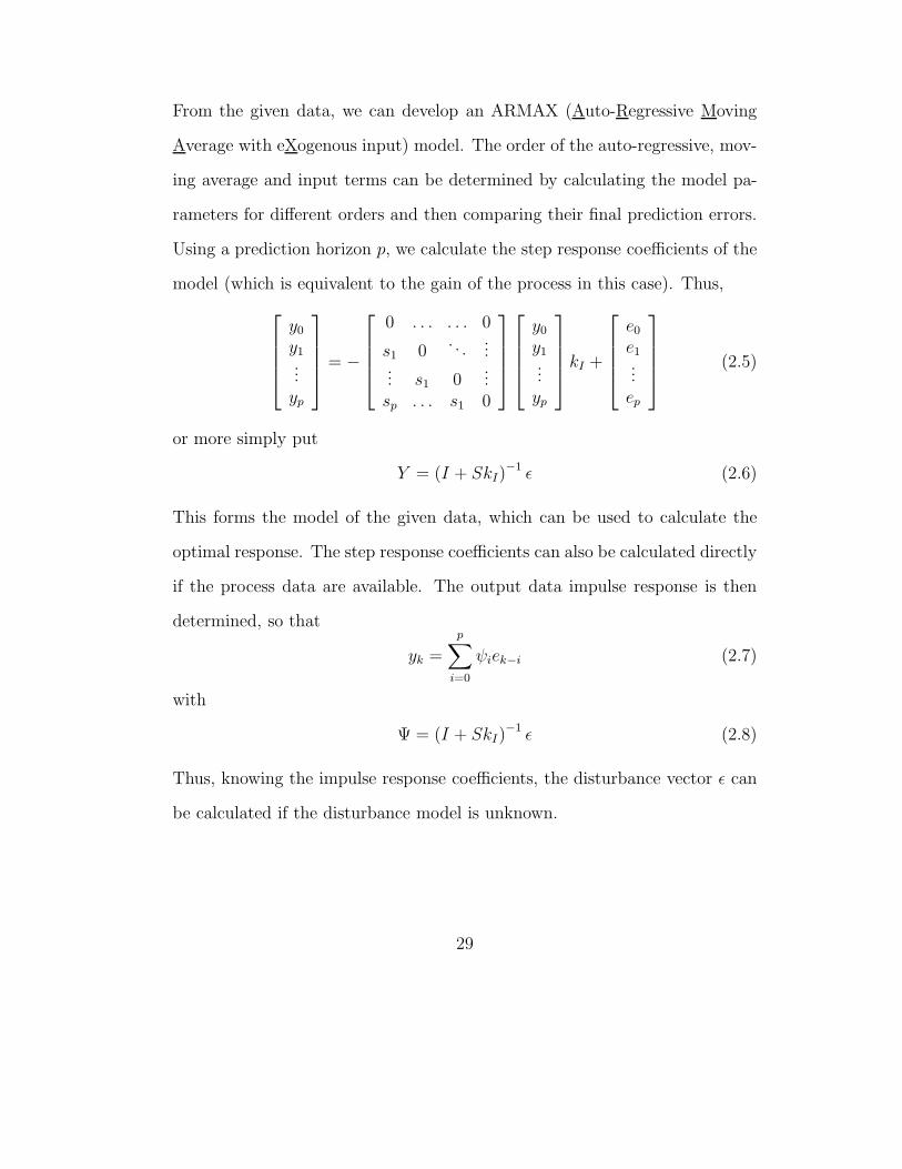
From the given data, we can develop an ARMAX (Auto-Regressive Moving

Average with eXogenous input) model. The order of the auto-regressive, mov-

ing average and input terms can be determined by calculating the model pa-

rameters for different orders and then comparing their final prediction errors.

Using a prediction horizon p, we calculate the step response coefficients of the

model (which is equivalent to the gain of the process in this case). Thus,

⎡⎢⎢⎢⎣y0

y1...yp

⎤⎥⎥⎥⎦ = −

⎡⎢⎢⎢⎣

0 . . . . . . 0

s1 0. . .

...... s1 0

...sp . . . s1 0

⎤⎥⎥⎥⎦⎡⎢⎢⎢⎣y0

y1...yp

⎤⎥⎥⎥⎦ kI +

⎡⎢⎢⎢⎣e0e1...ep

⎤⎥⎥⎥⎦ (2.5)

or more simply put

Y = (I + SkI)−1 ε (2.6)

This forms the model of the given data, which can be used to calculate the

optimal response. The step response coefficients can also be calculated directly

if the process data are available. The output data impulse response is then

determined, so that

yk =

p∑i=0

ψiek−i (2.7)

with

Ψ = (I + SkI)−1 ε (2.8)

Thus, knowing the impulse response coefficients, the disturbance vector ε can

be calculated if the disturbance model is unknown.

29

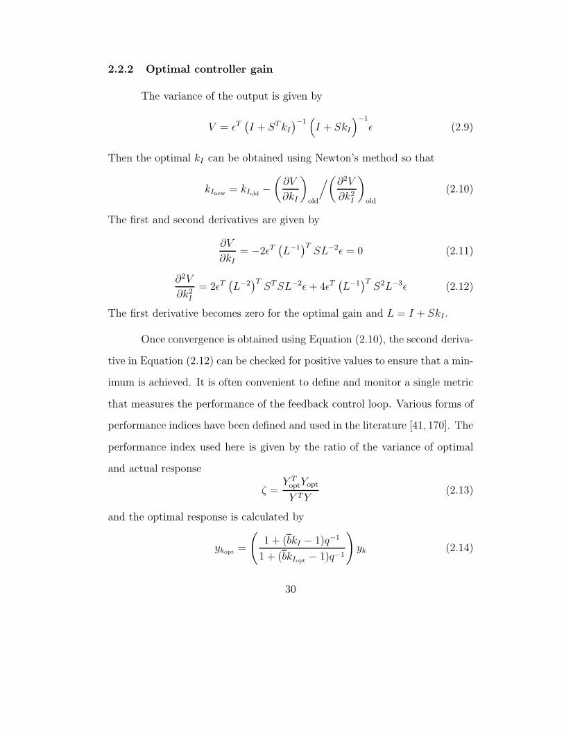
2.2.2 Optimal controller gain

The variance of the output is given by

V = εT(I + STkI

)−1(I + SkI

)−1

ε (2.9)

Then the optimal kI can be obtained using Newton’s method so that

kInew = kIold −(∂V

∂kI

)old

/(∂2V

∂k2I

)old

(2.10)

The first and second derivatives are given by

∂V

∂kI= −2εT

(L−1

)TSL−2ε = 0 (2.11)

∂2V

∂k2I

= 2εT(L−2

)TSTSL−2ε+ 4εT

(L−1

)TS2L−3ε (2.12)

The first derivative becomes zero for the optimal gain and L = I + SkI .

Once convergence is obtained using Equation (2.10), the second deriva-

tive in Equation (2.12) can be checked for positive values to ensure that a min-

imum is achieved. It is often convenient to define and monitor a single metric

that measures the performance of the feedback control loop. Various forms of

performance indices have been defined and used in the literature [41, 170]. The

performance index used here is given by the ratio of the variance of optimal

and actual response

ζ =Y T

optYopt

Y TY(2.13)

and the optimal response is calculated by

ykopt =

(1 + (bkI − 1)q−1

1 + (bkIopt − 1)q−1

)yk (2.14)

30

The normalized performance index has the range of 0 < ζ ≤ 1, and ζ = 1

indicates the best performance under integral control. With this definition,

1 − ζ indicates the maximum fractional reduction in the output variance.

2.2.3 EWMA Controller

The run-to-run system is controlled by a standard EWMA controller [23].

The equations are as follows (with similar notations): The actual process

yk = buk + ek (2.15)


yk = buk + ek (2.16)

We have assumed the bias term to be zero in this case. The observer updates

the disturbance using an EWMA formula, which is

ek+1 = λ(yk − buk+1) + (1 − λ)ek = λek + (1 − λ)ek (2.17)

The input is now given by (with ysp as the target)

uk+1 =ysp − ek+1

b(2.18)

The gain b is determined before the lot is processed using historical data.

For a pure gain system, the EWMA controller is equivalent to a discrete

integral controller (see Appendix A) with gain kI [18] such that

kI =λ

b(2.19)

31

Thus, by representing the closed-loop process as one controlled by a discrete

integral process, the performance index of an EWMA controlled process may

be obtained.

2.2.3.1 Equivalence to an internal model control (IMC) structure

Figure 2.1: IMC structure of an EWMA controller

Representing the existing EWMA controller in the run-to-run IMC

structure, as shown in Figure 2.1, the process and model transfer functions

will be

Gp = b (2.20)

and

Gm = b (2.21)

The equivalent IMC controller is

K =1

b(2.22)

with the EWMA filter as given in Equation (2.17).

32

2.2.3.2 Minimum mean squared error forecast

For an EWMA controller, the mean squared error of the forecast is

minimized if the disturbance is modeled by an integrated moving average time

series model (IMA) of the form:

ek+1 = ek + ak+1 − (1 − λ)ak (2.23)

where ak is a white noise sequence (See Appendix B for the proof). This fact

can be used for time-series modeling of the disturbance data in Equation (2.8)

and also to predict any missing observations in the data. The disturbance

sequence can be reconstructed from the time-series modeling of the sequence

and use to estimate the disturbance impulse response.

2.2.4 Sources of model error

The above model for the run-to-run controller may not represent the

system accurately in all aspects. As a result various kinds of mismatch may

occur, resulting in sub-optimal control. The point to be noted here is that

the controller has limited robustness in the face of model error and therefore

its performance is optimal given the existing uncertainties. Some of the as-

sumptions made in devising the plant model may not always hold. Here we

assume:

i. The process gain used is accurate and time-invariant (Gm = Gp).

ii. The disturbance follows the IMA (1,1) model as given in Equation (2.23).

33

iii. The EWMA parameter λ used is equivalent to the one apparent with

the IMA (1,1) disturbance model in Equation (2.23).

iv. There is no drift in the process, i.e., the process is stationary for the

given dataset under EWMA control.

v. No metrology delay is considered in the derivation. In actual practice,

the delay is almost always present for a typical process and often varies

according to process priority.

vi. It is assumed that the same tools are used for a single process. Data

from different tools is segregated in the form of threads.

vii. There is no set-point change during the time in which the process data

are evaluated.

2.3 Simulations

2.3.1 Data Analysis

The process needs to be identified with its parameters whenever we

calculate the performance index. Thus, for a given set of data we first identify

the model parameters using the simple gain model in Equation (2.16). The

disturbance model is similarly identified by differencing the values initially and

then using a first order moving average model. The process model and the

disturbance model are then used to calculate the step responses and impulse

responses respectively. If the process model is uncertain, advanced system

34

identification techniques [115] may be used to determine the correct model

orders for the process. These procedures usually produce model estimates for

all possible model order combinations in a ARMAX setup. Following this, the

model that best explains the given data is chosen viz. the unexplained variance

is lowest for that model. Model complexity may be restricted by penalizing

higher number of parameters using the final prediction error criterion.

2.3.1.1 Moving Window

In calculating the performance of the EWMA controller, it is important

to determine how much past data needs to be considered. For this purpose

we use a moving window of data, i.e., we only use data from the last n lots to

be run, where n is the moving window size. This restriction helps to calculate

a performance index that is current and can be incorporated into an on-line

tool without too much computational power being consumed in the analysis.

The choice of moving window size is not simple since it demands a trade-off

between maximizing the use of available data and minimizing the computation

time required. In general, we use the principle that the window size should not

be less than what is needed to produce a good estimate of the model. It should

also not be too large, not just to save computational time but also to avoid

changes in the process being smoothed out in the identification procedure.

35

2.3.1.2 Effect of moving window size

In general we specify a minimum moving window size of 20 in order

to obtain good model estimates. But small window sizes also lead to another

peculiar effect, which is the variation of the performance index about its mean.

The statistical properties of the performance index ζ can be seen in the original

paper by Ko and Egdar [101]. To observe the effect of the moving window size

on the variation in performance index, we set up a simulation as follows. A

run-to-run process following the correct models is used so that the performance

index is unity at all times on average. The process parameters of λ = 0.3 and

δ = 1 are used along with unity white noise variance. A sample size of 100

is used and the moving window size is varied from 20 to 90 in increments of

10. 10 values of performance index are calculated at each window size and

the standard deviation is noted. The results can be seen in Figure (2.2).

We observe that the standard deviation declines in inverse proportion to the

moving window size. Thus we can define the moving window size to be the one

which is greater than the minimum required for identification but with which

the variation in performance index is tolerable. Let this tolerance be 1% of

the performance index or 0.01. From Figure (2.2) we fix our moving window

to a size of at least 50 henceforth.

2.3.2 Model mismatch

As seen from the process model, accurate knowledge of the model pa-

rameters determines whether the process is optimal. We define this accuracy

36

in terms of δ, which is the ratio of the actual gain to the gain used by the

run-to-run controller and θ, the parameter for the IMA(1,1) model. Ideally,

we need these parameters to be as accurate as possible. But invariably, the

value of δ deviates from unity, affecting in turn, the performance of the EWMA

controller because of gain mismatch. Also, the EWMA parameter λ used may

not accurately reflect the true value needed based on λ = 1−θ. Let us consider

the possible cases of gain mismatch and disturbance model mismatch that can

occur in manufacturing in order to quantify their effect on the performance

index.

20 30 40 50 60 70 80 900

0.01

0.02

0.03

0.04

0.05

0.06

0.07

Moving Window Size

Sta

ndar

d D

evia

tion

of P

erfo

rman

ce In

dex

Figure 2.2: Variation in performance index with moving window size. A declinein the standard deviation of the performance index is observed with increasingmoving window size.

37

2.3.2.1 Effect of gain mismatch

The first type of model mismatch that can occur is an absolute gain

mismatch. This means that the value of δ is constant but not equal to one.

This may occur in particular when the gain used is based on a calculation

from historical process data. We now simulate a run-to-run process with the

correct disturbance model (λ = 0.3) but vary the gain ratio δ from 0.5 to 1.5

in increments of 0.1. This range is typical for the processes under considera-

tion and lies within the stability limits of the system [58]. This simulation is

repeated 100 times for each value of δ to smooth out the performance index.

0.5 0.6 0.7 0.8 0.9 1 1.1 1.2 1.3 1.4 1.50

0.2

0.4

0.6

0.8

1

1.2

Actual Gain / Gain used

Mea

n P

erfo

rman

ce In

dex

Mean PIUpper BoundLower Bound

Figure 2.3: Effect of absolute gain mismatch on the performance index of asimulated run-to-run EWMA controlled process. The EWMA parameter λused is accurate and equal to 0.3. The performance index falls rapidly withhigher values of gain mismatch.

38

Figure (2.3) shows the change in performance index with absolute gain

mismatch. It also shows the upper and lower bounds on the performance index

based on their deviations from the mean. We can see that the effect of gain

mismatch is drastic on the performance of an EWMA system. The index is

close to 1 only when the value of δ is very close to unity. The performance

index falls rapidly with further deviation of δ from unity. It also increases

the variation of performance index over a fixed period of time. Thus we may

conclude that a very low performance index may indicate a mismatch in the

gain of the process. Note that typical δ values lie between 0.8 and 1.2 whenever

gains are based on historical data.

2.3.2.2 Effect of error in disturbance parameter

We now look at the impact of an error in the optimal and actual value

of the EWMA parameter λ used in the process. We know that for a given

value θ for the IMA(1,1) disturbance model, the optimal value of the EWMA

parameter is λ = 1 − θ. An EWMA filter with λ = 0.5 is now used in

a simulated run-to-run process with no gain mismatch, viz. δ = 1. The

value of θ is now varied from 0 to 0.9. Thus, the mismatch λ − λopt varies

from -0.5 to 0.4. Note that a value of θ = 0 implies a random walk model.

This simulation is repeated 100 times for each value of θ to smooth out the

performance index. Figure (2.4) shows the change in performance index with

change in mismatch of the disturbance parameter. It is seen that at negative

mismatch, the performance index decreases to a larger extent than at positive

39

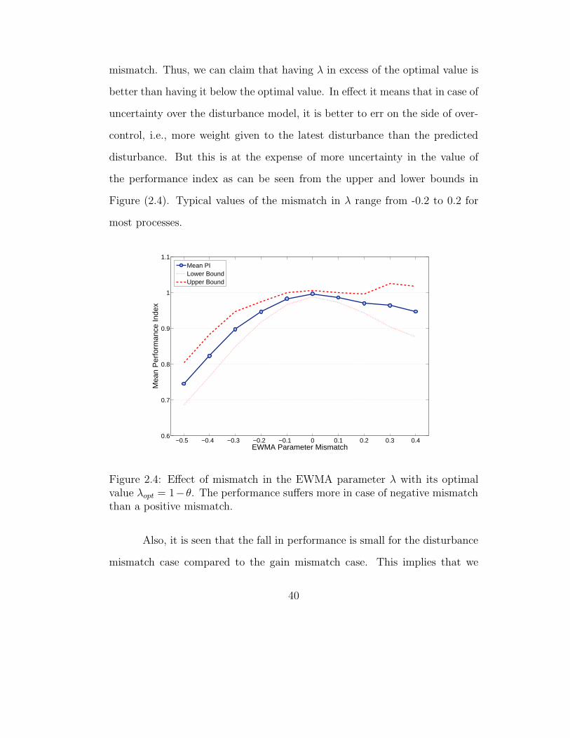
mismatch. Thus, we can claim that having λ in excess of the optimal value is

better than having it below the optimal value. In effect it means that in case of

uncertainty over the disturbance model, it is better to err on the side of over-

control, i.e., more weight given to the latest disturbance than the predicted

disturbance. But this is at the expense of more uncertainty in the value of

the performance index as can be seen from the upper and lower bounds in

Figure (2.4). Typical values of the mismatch in λ range from -0.2 to 0.2 for

most processes.

−0.5 −0.4 −0.3 −0.2 −0.1 0 0.1 0.2 0.3 0.40.6

0.7

0.8

0.9

1

1.1

EWMA Parameter Mismatch

Mea

n P

erfo

rman

ce In

dex

Mean PILower BoundUpper Bound

Figure 2.4: Effect of mismatch in the EWMA parameter λ with its optimalvalue λopt = 1−θ. The performance suffers more in case of negative mismatchthan a positive mismatch.

Also, it is seen that the fall in performance is small for the disturbance

mismatch case compared to the gain mismatch case. This implies that we

40

favor accuracy of the process gain over the accuracy of the EWMA parameter

λ.

2.3.3 Effect of delay

So far we have neglected an important aspect of any controlled process,

which is the presence of delays which hinder the measurements from reaching

the controller at the right time to make an impact. Such delays are always

present in any semiconductor manufacturing process and need to be accounted

for. We therefore consider the impact of two types of delays that may result in

this scenario. One type of delay is inherent in a process and is therefore called

a process delay. The other type results due to constraints in the metrology or

measurement of wafers and is therefore referred to as a metrology delay.

2.3.3.1 Effect of process delays

A process may have an inherent delay which allows the input to affect

the output only after a specified number of runs. Since the process is run-to-

run, we only have integral delays in this case. This may occur when the wafer

cannot be measured until after a certain set of processing steps have occurred

after the run or when a specific uniform sampling strategy is used to reduce

metrology costs. We consider the case where there is no model mismatch for

the run-to-run EWMA controlled process but there is a constant delay which

is not considered in the model. A large value of 200 is used for the moving

window size and only a single performance index value is calculated for the

41

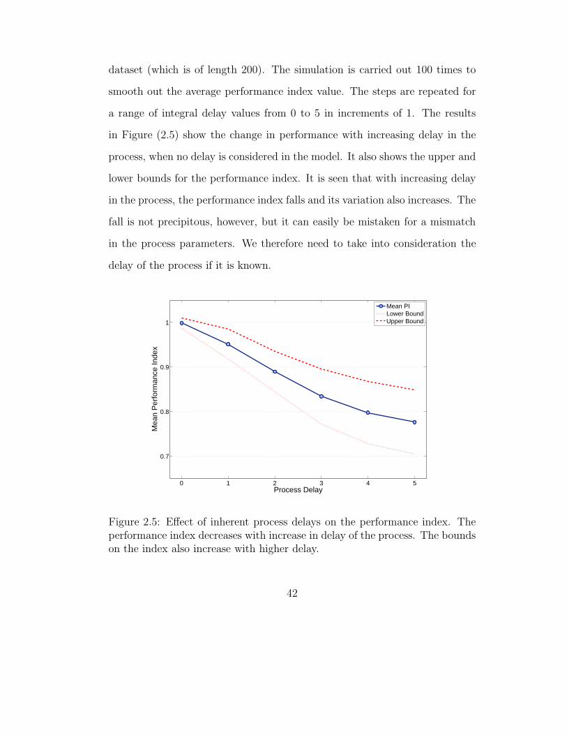
dataset (which is of length 200). The simulation is carried out 100 times to

smooth out the average performance index value. The steps are repeated for

a range of integral delay values from 0 to 5 in increments of 1. The results

in Figure (2.5) show the change in performance with increasing delay in the

process, when no delay is considered in the model. It also shows the upper and

lower bounds for the performance index. It is seen that with increasing delay

in the process, the performance index falls and its variation also increases. The

fall is not precipitous, however, but it can easily be mistaken for a mismatch

in the process parameters. We therefore need to take into consideration the

delay of the process if it is known.

0 1 2 3 4 5

0.7

0.8

0.9

1

Process Delay

Mea

n P

erfo

rman

ce In

dex


Figure 2.5: Effect of inherent process delays on the performance index. Theperformance index decreases with increase in delay of the process. The boundson the index also increase with higher delay.

42

Figure (2.6) shows the change in performance index with the delay con-

sidered. We simulate a process as before but fix the inherent delay to 3. The

delay considered in the model is now increased from 0 to 4 in increments of

1. We observe that the performance index rises as the accuracy of the delay

considered in the model increases. The bounds on the index also correspond-

ingly decrease. With further increases in the delay beyond the actual value,

no change is observed.

0 1 2 3 40.7

0.8

0.9

1

1.1

Model Delay

Mea

n P

erfo

rman

ce In

dex


Figure 2.6: Change in performance index with delay considered in the model.The original process has a constant delay of 3. The index stays low until thedelay considered is close to the actual value.

43

2.3.3.2 Effect of metrology delays

Another type of delay which is usually present in such systems is the

metrology delay. Since the input for each run depends on the value of the

output for the previous run, we need to measure the wafer after every run. But

in any semiconductor fabrication facility, there are multiple processes occurring

in any given time period. The metrology equipment being expensive in most

cases is used optimally. As a result, there is a backlog of wafers waiting to be

measured. The measurement also takes place by priority, i.e., the most critical

wafers are measured first. This delay is again an integer but it is no longer

constant. In most cases it varies from 0 to 5 with a mean delay of 1 or 2. Higher

delays are rare since it usually sounds an alarm to the operator to measure a

wafer. We therefore simulate different cases of such metrology induced delays

to observe its impact on the process. A run-to-run EWMA controlled process

with no model mismatch is simulated with no inherent process delay. There

is, however, a variable metrology delay which varies from 0 to 3. A moving

window size of 50 is used and 50 values of performance index are calculated for

each simulation. The delay mode (i.e., the delay which occurs most frequently)

is changed from 0 to 3. The simulations are repeated 10 times for each of the

four delay cases. The results are shown in Table (2.1). The table shows a

general decline in the performance with increasing delay mode but the effect

is subdued and relates directly to the mean value of the delay. Again, this

muddles the picture in case of determining the process optimality since the

performance index reflects the processing constraints rather than the process

44

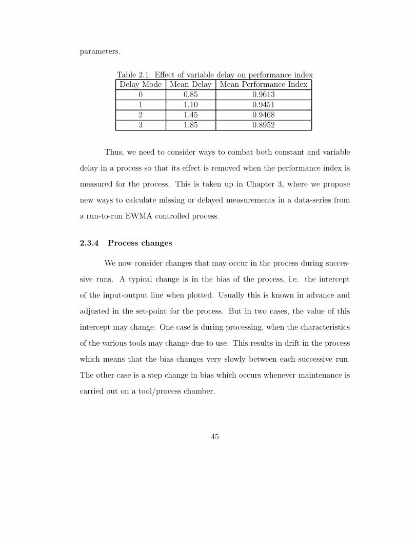
parameters.

Table 2.1: Effect of variable delay on performance indexDelay Mode Mean Delay Mean Performance Index

0 0.85 0.96131 1.10 0.94512 1.45 0.94683 1.85 0.8952

Thus, we need to consider ways to combat both constant and variable

delay in a process so that its effect is removed when the performance index is

measured for the process. This is taken up in Chapter 3, where we propose

new ways to calculate missing or delayed measurements in a data-series from

a run-to-run EWMA controlled process.

2.3.4 Process changes

We now consider changes that may occur in the process during succes-

sive runs. A typical change is in the bias of the process, i.e. the intercept

of the input-output line when plotted. Usually this is known in advance and

adjusted in the set-point for the process. But in two cases, the value of this

intercept may change. One case is during processing, when the characteristics

of the various tools may change due to use. This results in drift in the process

which means that the bias changes very slowly between each successive run.

The other case is a step change in bias which occurs whenever maintenance is

carried out on a tool/process chamber.

45

2.3.4.1 Effect of time-varying bias

The bias may change over time due to change in processing conditions

over successive runs. For example, reactor chamber walls may get fouled over

time. As a result, the bias may show a steady change which is noticeable

only over a long period of time. It can be detected by plotting the output

versus the input and observing the change in intercept. We simulate such a

process where the increase in bias occurs very slowly, at 0.1 units per run. The

set-point for the process is 10 and λ = 0.3. The length of the time-series is

200 and a moving window size of 50 is used. We calculate 150 values of the

performance index thus covering the entire dataset from set 1-50 to 151-200.

Also, we state that the drift is detected at run 125 and is reset to its original

value. Figure (2.7) now shows the trend in performance index over each run.

We see that at run 50, the index is already below 0.8, suggesting the influence

of drifting bias. As the bias drifts further, the performance suffers even more,

reaching lows of 0.2 at run 125. Since the bias gets reset at run 125, an increase

is observed subsequently. Then at around run 175, since the moving window

is 50, the bias effect disappears completely from the dataset. This is indicated

by the index moving abruptly to the optimal value of unity towards then end.

Thus, we observe that the drift in bias, if undetected, can lead to a drastic

drop in performance. Any maintenance carried out to remove its effect makes

the process optimal once again.

46

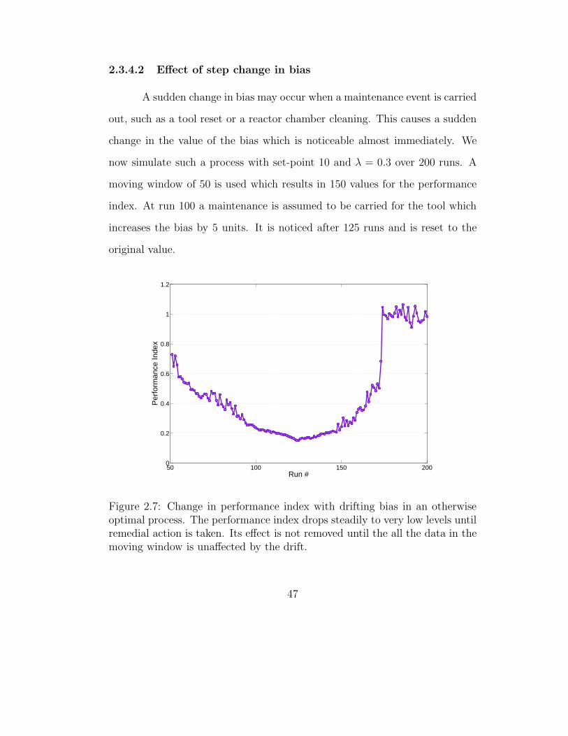
2.3.4.2 Effect of step change in bias

A sudden change in bias may occur when a maintenance event is carried

out, such as a tool reset or a reactor chamber cleaning. This causes a sudden

change in the value of the bias which is noticeable almost immediately. We

now simulate such a process with set-point 10 and λ = 0.3 over 200 runs. A

moving window of 50 is used which results in 150 values for the performance

index. At run 100 a maintenance is assumed to be carried for the tool which

increases the bias by 5 units. It is noticed after 125 runs and is reset to the

original value.

50 100 150 2000

0.2

0.4

0.6

0.8

1

1.2

Run #

Per

form

ance

Inde

x

Figure 2.7: Change in performance index with drifting bias in an otherwiseoptimal process. The performance index drops steadily to very low levels untilremedial action is taken. Its effect is not removed until the all the data in themoving window is unaffected by the drift.

47

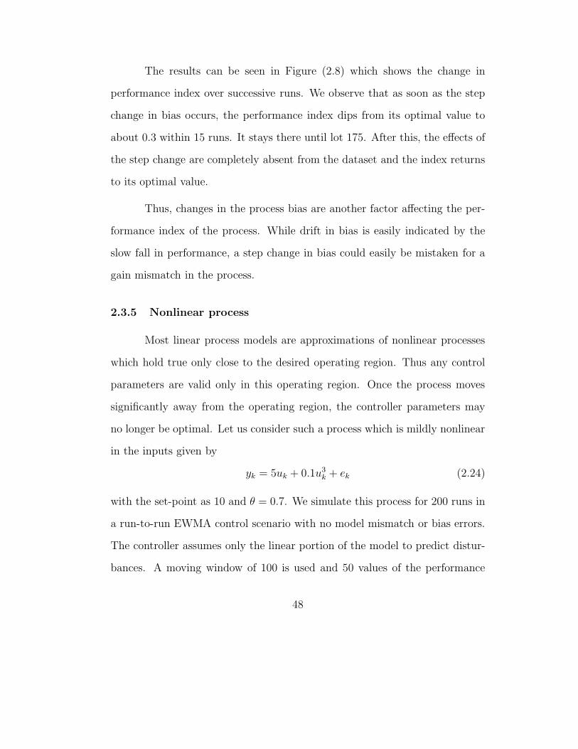
The results can be seen in Figure (2.8) which shows the change in

performance index over successive runs. We observe that as soon as the step

change in bias occurs, the performance index dips from its optimal value to

about 0.3 within 15 runs. It stays there until lot 175. After this, the effects of

the step change are completely absent from the dataset and the index returns

to its optimal value.

Thus, changes in the process bias are another factor affecting the per-

formance index of the process. While drift in bias is easily indicated by the

slow fall in performance, a step change in bias could easily be mistaken for a

gain mismatch in the process.

2.3.5 Nonlinear process

Most linear process models are approximations of nonlinear processes

which hold true only close to the desired operating region. Thus any control

parameters are valid only in this operating region. Once the process moves

significantly away from the operating region, the controller parameters may

no longer be optimal. Let us consider such a process which is mildly nonlinear

in the inputs given by

yk = 5uk + 0.1u3k + ek (2.24)

with the set-point as 10 and θ = 0.7. We simulate this process for 200 runs in

a run-to-run EWMA control scenario with no model mismatch or bias errors.

The controller assumes only the linear portion of the model to predict distur-

bances. A moving window of 100 is used and 50 values of the performance

48

index are calculated. This process is repeated multiple times so that different

regions of the input values are exposed.

50 100 150 2000

0.2

0.4

0.6

0.8

1

1.2

Run #

Per

form

ance

Inde

x

Figure 2.8: Change in performance index with step change in bias in an oth-erwise optimal process. The index drops immediately to a lower value oncethe step change takes place. It does not recover until the bias is reset and ithas no effect on the moving window under consideration.

Figure (2.9) shows the trends in performance index for three different

operating regions. We observe very different behavior depending on the input

values, due to the presence of nonlinearities. In the first case, the process

is nearly optimal and the performance is steady. In the second case, the

performance index is low but it slowly increases over successive runs. In the

third case, however, the index is already low and it falls even further with each

run. So for the same process we get multiple values for the performance index

49

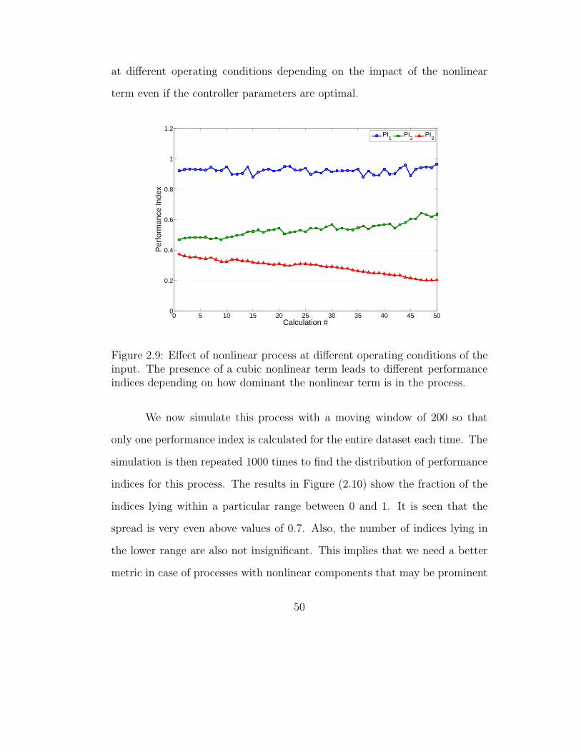
at different operating conditions depending on the impact of the nonlinear

term even if the controller parameters are optimal.

0 5 10 15 20 25 30 35 40 45 500

0.2

0.4

0.6

0.8

1

1.2

Calculation #

Per

form

ance

Inde

x

PI1

PI2

PI3

Figure 2.9: Effect of nonlinear process at different operating conditions of theinput. The presence of a cubic nonlinear term leads to different performanceindices depending on how dominant the nonlinear term is in the process.

We now simulate this process with a moving window of 200 so that

only one performance index is calculated for the entire dataset each time. The

simulation is then repeated 1000 times to find the distribution of performance

indices for this process. The results in Figure (2.10) show the fraction of the

indices lying within a particular range between 0 and 1. It is seen that the

spread is very even above values of 0.7. Also, the number of indices lying in

the lower range are also not insignificant. This implies that we need a better

metric in case of processes with nonlinear components that may be prominent

50

under some conditions. We explore this issue in more detail in Chapter 5.

<0.1 0.1−0.2 0.2−0.3 0.3−0.4 0.4−0.5 0.5−0.6 0.6−0.7 0.7−0.8 0.8−0.9 >0.90

0.05

0.1

0.15

0.2

0.25

Range of Performance Index

Pro

babi

lity

Figure 2.10: The distribution is uniform at both the higher and lower end ofoptimality. The index varies according to the value of the inputs.

2.4 Results from manufacturing data

We now apply the performance monitoring method for EWMA con-

trollers developed earlier to actual fab data from AMD1. A total of three

different processes are considered, two types of etch processes and an expo-

sure process. Each of these processes is threaded, i.e., the data streams are

segregated based on the product, layer, tool and any other such factor which

is known to influence the process disturbance. We analyze these threads indi-

1Advanced Micro Devices, Inc.

51

vidually with a moving window of 50 and 50 calculations of the performance

index. As a consequence, of all the threads present in the system, we only

analyze those which have at least 100 data-points. Thus, the results provide a

snapshot of the current state of the processes by means of the performance dis-

tribution plots and plots of performance changes over time for select threads.

2.4.1 Etch process A

We first consider a shallow trench isolation (STI) etch process for per-

formance monitoring and analysis. The process model used for this process is

as follows

EtchDepth = EtchRate× EtchT ime+Bias (2.25)

The Bias is updated by EWMA as given in the previous sections. Accord-

ingly, the manipulated variable is EtchT ime, while the controlled variable is

EtchDepth. The data from this process is further segregated into 47 threads

with different settings for the EtchRate in each case.

2.4.1.1 Distribution of performance indices

We calculate 50 values of the performance index using a moving window

of 50 for each of the 47 threads. In order to observe the overall performance of

this process, we plot the distribution of all the performance index values (2350

total) over the complete range of performance indices from 0 to 1. Figure (2.11)

shows the fraction of values lying within the given range. It is seen that about

80% of the values are above 0.9. Thus 20% of the values lie in the sub-optimal

52

range.

0−0.1 0.1−0.2 0.2−0.3 0.3−0.4 0.4−0.5 0.5−0.6 0.6−0.7 0.7−0.8 0.8−0.9 >0.90

0.2

0.4

0.6

0.8

1


Fra

ctio

n of

Indi

ces

Figure 2.11: Distribution of performance indices for Etch A.

2.4.1.2 Sample thread performance plots

Figures (2.12) to (2.16) showcase the change in performance over time

for five different threads. While threads 1, 3 and 4 show a sudden drop in

performance index, threads 2 and 5 show a slow drop in the metric. The

former indicates step changes in the bias due to maintenance events, while

the latter is more likely to be due to a drift in the bias. Figure (2.15) also

shows the average bias over the moving window at every calculation. As seen

in the figure, the increase in bias can be roughly correlated with the drop in

performance index.

53

0 5 10 15 20 25 30 35 40 45 500.4

0.5

0.6

0.7

0.8

0.9

1

1.1

Calculation #

Per

form

ance

Inde

x

Figure 2.12: Change in performance index over time for Thread 1 in Etch A.

0 5 10 15 20 25 30 35 40 45 500.4

0.5

0.6

0.7

0.8

0.9

1

1.1

Calculation #

Per

form

ance

Inde

x


54

2.4.2 Etch process B

We now consider a polygate etch process for performance monitoring

and analysis. The following process model is used

DICD − FICD = Slope×EtchT ime+Bias (2.26)

Here DICD is the width of the resist line (feedback variable) while FICD is

the width of the gate (feedforward variable). The Bias is updated using an

EWMA filter. The manipulated variable here is EtchT ime, while DICD is

the controlled variable. The data from this process is further segregated into

19 threads, with different values for the Slope in each case.

0 5 10 15 20 25 30 35 40 45 500.4

0.5

0.6

0.7

0.8

0.9

1

1.1

Calculation #

Per

form

ance

Inde

x


55






shows the fraction of values lying within the given range. It is seen that almost

90% of the values are above 0.9. Thus etch process B shows a better overall

performance than etch process A.

0 10 20 30 40 500.6

0.7

0.8

0.9

1

1.1

1.2

Calculation #

Per

form

ance

Inde

x

0 10 20 30 40 500

0.5

1

1.5

Calculation #

Ave

rage

bia

s ov

er m

ovin

g w

indo

w

3

3

2

1

1 2

Figure 2.15: Change in performance index over time for Thread 4 in Etch A.The regions correspond to changes in the bias and its effect on the performanceindex. (1) shows an increase in bias to 1. (2) shows a large drop in performancewhen the bias increases from 1 to 1.5. (3) shows an increase in performancefor a brief period when the bias falls in value.

56

0 5 10 15 20 25 30 35 40 45 500.4

0.5

0.6

0.7

0.8

0.9

1

1.1

Calculation #

Per

form

ance

Inde

x


0−0.1 0.1−0.2 0.2−0.3 0.3−0.4 0.4−0.5 0.5−0.6 0.6−0.7 0.7−0.8 0.8−0.9 >0.90

0.2

0.4

0.6

0.8

1


Fra

ctio

n of

Indi

ces

Figure 2.17: Distribution of performance indices for Etch B.

57


Figures (2.18) to (2.20) showcase the change in performance over time

for three different threads. The first shows a near optimal process with aver-

age performance index close to 1. The second shows an already sub-optimal

process, degrading even further over at the very end. This indicates a possi-

ble model mismatch compounded by a possible drifting bias towards the end.

The third is a similar case, except that the drift in bias is apparent from the

beginning of the runs under consideration. As a result, the performance index

falls to almost 0.5 towards the end.

0 5 10 15 20 25 30 35 40 45 500.4

0.5

0.6

0.7

0.8

0.9

1

1.1

Calculation #

Per

form

ance

Inde

x

Figure 2.18: Change in performance index over time for Thread 1 in Etch B.

58

0 5 10 15 20 25 30 35 40 45 500.4

0.5

0.6

0.7

0.8

0.9

1

1.1

Calculation #

Per

form

ance

Inde

x


0 5 10 15 20 25 30 35 40 45 500.4

0.5

0.6

0.7

0.8

0.9

1

1.1

Calculation #

Per

form

ance

Inde

x


59

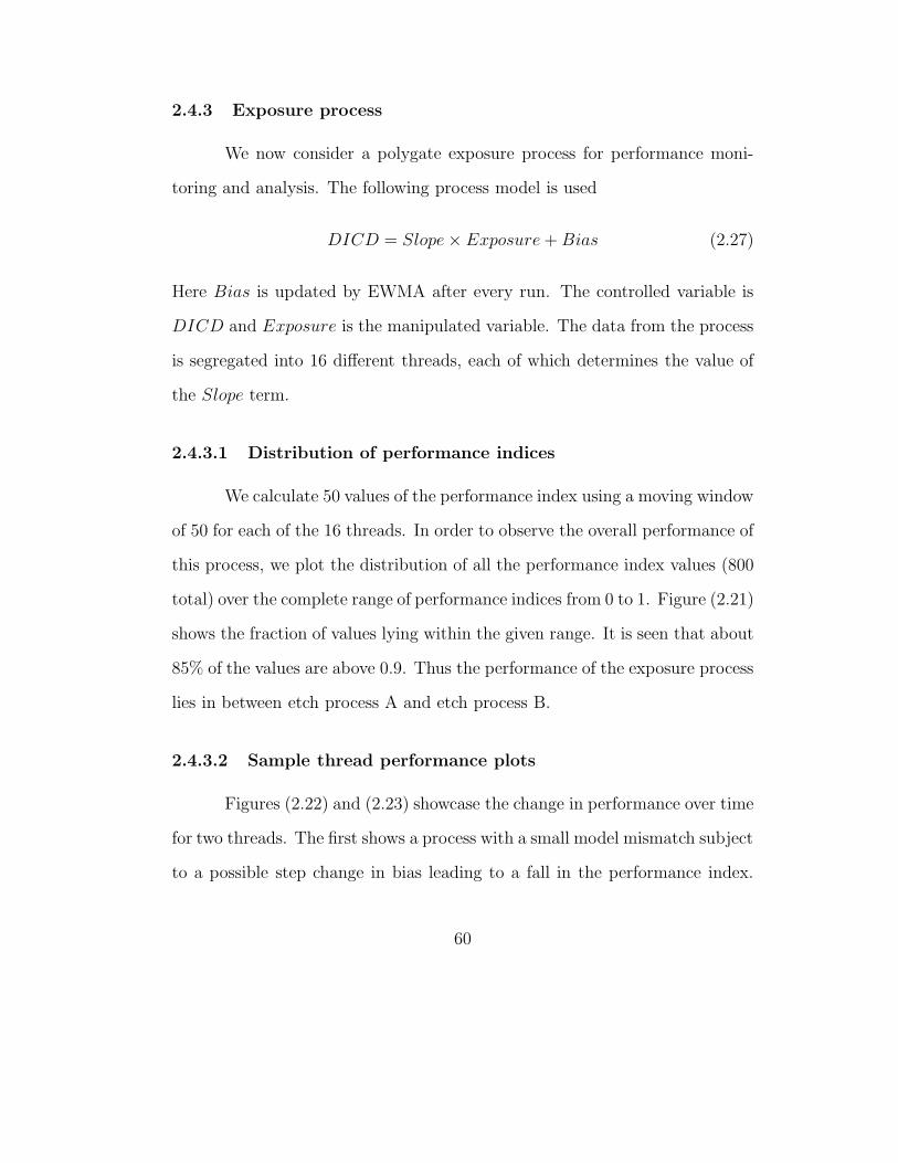
2.4.3 Exposure process

We now consider a polygate exposure process for performance moni-

toring and analysis. The following process model is used

DICD = Slope× Exposure+Bias (2.27)

Here Bias is updated by EWMA after every run. The controlled variable is

DICD and Exposure is the manipulated variable. The data from the process

is segregated into 16 different threads, each of which determines the value of

the Slope term.






shows the fraction of values lying within the given range. It is seen that about

85% of the values are above 0.9. Thus the performance of the exposure process

lies in between etch process A and etch process B.


Figures (2.22) and (2.23) showcase the change in performance over time

for two threads. The first shows a process with a small model mismatch subject

to a possible step change in bias leading to a fall in the performance index.

60

The second shows a near optimal process which is seen to degrade at the very

end.

2.5 Conclusions and future work

In this chapter, performance metric was proposed for use in assessing

and monitoring single-loop EWMA control performance. For this purpose, an

iterative solution was derived that gives the best achievable performance in

terms of the closed-loop input-output data and the process model. An explicit

solution was derived as a function of EWMA parameter λ and the process gain

b. A performance index was defined based on the best achievable performance

for use as a realistic performance measure in the single-loop EWMA control

0−0.1 0.1−0.2 0.2−0.3 0.3−0.4 0.4−0.5 0.5−0.6 0.6−0.7 0.7−0.8 0.8−0.9 >0.90

0.2

0.4

0.6

0.8

1


Fra

ctio

n of

Indi

ces

Figure 2.21: Distribution of performance indices for the exposure process.

61

system.

0 5 10 15 20 25 30 35 40 45 500.4

0.5

0.6

0.7

0.8

0.9

1

1.1

Calculation #

Per

form

ance

Inde

x

Figure 2.22: Change in performance index over time for Thread 1 in theexposure process.

It was observed from simulations that a higher moving window size led

to smaller variations in the performance index value, leading to an optimal

window size selection. Gain mismatch was found to have a larger impact on

the performance of the process as compared to a mismatch in the EWMA fil-

ter parameter. Process and metrology delays were found to have a significant

impact on the performance of the EWMA controller and therefore need to

be accounted for or corrected in order to minimize their impact on the per-

formance. Bias effects are also prominent as seen from the simulations with

drifting bias and step changes in bias. Nonlinearity on the process was found

62

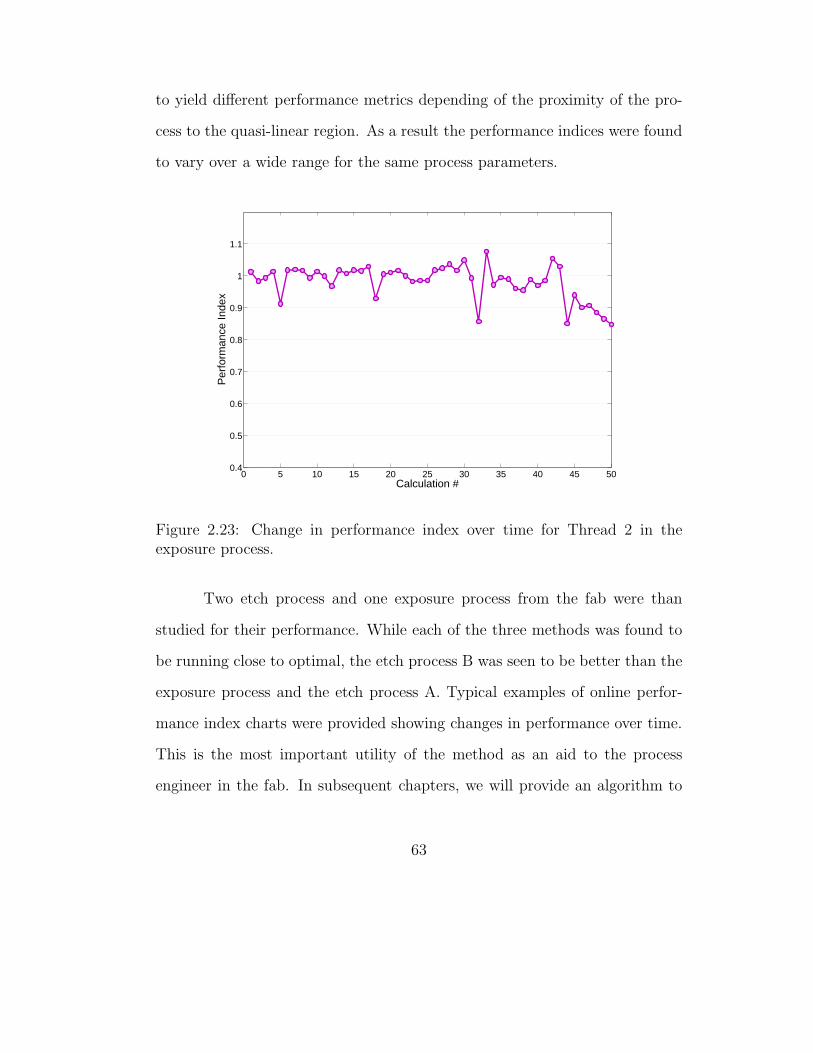
to yield different performance metrics depending of the proximity of the pro-

cess to the quasi-linear region. As a result the performance indices were found

to vary over a wide range for the same process parameters.

0 5 10 15 20 25 30 35 40 45 500.4

0.5

0.6

0.7

0.8

0.9

1

1.1

Calculation #

Per

form

ance

Inde

x

Figure 2.23: Change in performance index over time for Thread 2 in theexposure process.

Two etch process and one exposure process from the fab were than

studied for their performance. While each of the three methods was found to

be running close to optimal, the etch process B was seen to be better than the

exposure process and the etch process A. Typical examples of online perfor-

mance index charts were provided showing changes in performance over time.

This is the most important utility of the method as an aid to the process

engineer in the fab. In subsequent chapters, we will provide an algorithm to

63

compensate for the variable and constant delay in the process (Chapter 3),

measure performance in case of non-threaded control (Chapter 4), and pro-

vide a unique metric which takes the nonlinearity of the process into account

(Chapter 5).

64

Chapter 3

Missing Data Estimation for Run-to-Run

EWMA-controlled Processes

3.1 Introduction

Missing data is a common problem in automatic control in the process

industries. This is especially true in semiconductor manufacturing, where the

output measurements, or metrology, are carried out separately from the pro-

cess equipment [46]. Run-to-run control is the most popular form of feedback

control in semiconductor manufacturing, wherein the manipulated variables

are adjusted after each lot, based on the data from the previous lot. Often

the processing and metrology sequences do not match, and some data always

tends to be missing. Also, not all wafers in a lot are measured; rather some

fraction is measured based on a predetermined sampling strategy. This creates

a problem because the controller outputs are updated using measurements of

previous process outputs. In actual practice, this problem is often ignored

and controller outputs are updated based on available data. This chapter pro-

poses a method to obtain optimal estimates of the missing data. The purpose

of determining the missing values is two-fold: one is providing a method to

reconstruct data from an EWMA-controlled process, where it is known that

some lots were run with missing data. Another is providing reliable forecasts

65

to enable feedforward control on processes with less than 100% metrology.

3.1.1 Choice of estimation method

The choice of an appropriate method for handling missing data depends

in part on the cause of the missing data. Rubin’s classic paper [154] developed

the following classifications of missing data:

a. Data are missing completely at random (MCAR) if the observations with

any missing values are a random subsample of the full sample. This

means that the distribution of missing values does not depend on either

the missing values or the observed values. In this case, the missing-data

mechanism is unrelated to the model and therefore can be ignored.

b. Data are missing at random (MAR) if the missing pattern for a variable

is not a function of the missing values, but may be a function of the

observed values in the model. MAR is a less stringent assumption than

MCAR.

c. Values are classified as not missing at random (NMAR) if they are sys-

tematically missing from the data set, i.e., the missingness is a function

of the values that are missing. In a time series, this might mean that

the missing data occur in patterns, are related to the numeric values of

the series, or may be considered as outliers.

These definitions were further clarified in the literature [71, 86, 160] over the

last few years.

66

In semiconductor manufacturing, there may be specific patterns of miss-

ing data in particular if a sampling strategy is used during metrology, i.e., less

than 100% of the wafers (or lots) are sampled, or when there is high demand

for limited metrology tools leading to the scenario where lots or wafers may be

processed before the measurement for the previous run is available. Both these

cases may be classified as MCAR and therefore the model may be estimated

from available data in such cases. There are also cases where the missing data

may be MAR, such as when the metrology gives preference to a wafer based

on a specific product line or if the wafers undergo adaptive sampling based

on observed values. The only NMAR case of missing data in semiconduc-

tor manufacturing occurs when data are classified as outliers based on SPC

principles.

There are several methods that treat a time-series with missing output

values. These methods can be ad hoc or rigorous techniques and are listed

below:

a. Ignore the missing observations: The first ad hoc procedure for handling

missing data is deletion, that is, eliminating the observations that are

missing from the series and then analyzing the condensed series as if it

were the same as an original shorter series. This is the most direct route

to deal with missing data in a time-series. The costs associated with

using deletion include (1) the method will always decrease the sample

size and (2) the method can lead to biased parameter estimates if the

data are not MCAR. As a rule of thumb, if the fraction of missing data

67

is less than 10 to 15%, one can neglect the missing points and proceed

with the data analysis assuming that those points will have little or no

effect on the estimation of the model. However, with larger fractions of

missing data, it is desirable to produce estimates for the missing values

since the model uncertainty would increase if they are neglected.

b. Substitute the missing value: The second ad hoc technique involves sub-

stituting the mean of the series or the target value of the output for the

missing value. In the first case, the mean would be obtained from all of

the non-missing observations in a time-series, and that value would be

assigned for each missing observation. This method ignores the order of

the observations. With respect to the estimation of dependency, assign-

ing the mean values may inappropriately smooth a series with negative

autocorrelation. Simply using mean values can provide inaccurate esti-

mates when there is a nonzero slope in the series. The appeal of this

method is simplicity, hence its widespread use. Similarly, substituting

the target value of the output can be used when the process is under

control. As with the mean, this may smooth the time-series and lead to

inaccurate model estimates.

c. Use the mean of adjacent observations: The third ad hoc technique in-

volves substituting the mean of the adjacent observations for any miss-

ing data. This method takes into account the order of the observations.

The mean of the adjacent observations should be more accurate when

68

the slope of a series is non-zero. Assigning the mean of the adjacent ob-

servations may also be more accurate than the mean of the entire series

when the autocorrelation is positive. However, when it is negative, using

the mean of the adjacent observations may artificially smooth the series

and mask the amount of autocorrelation actually present in the behavior

of interest.

d. Use the estimate obtained using techniques such as Kalman smoothing

or expectation maximization algorithms. Most of these methods are

geared towards identification of a time-series by first classifying the type

of model that it is supposed to fit. The missing data is then estimated,

usually by some form of a smoothing algorithm. The model is then

estimated using maximum likelihood techniques.

3.1.2 Existing literature

Over the years there have been many articles in literature dealing with

the problem of missing data estimation. Most methodologies solve the miss-

ing data problem as a step towards a larger goal: identification of the process

model. Other methodologies deal with a specific time series model such as an

autoregressive (AR), autoregressive moving average (ARMA) or autoregres-

sive integrated moving average (ARIMA) model. The problem has appeared

mostly in the field of statistical economics [102] but also in communication

networks [164] and for identification and control [89].

Wilkinson [189] was one of the first to consider this problem and pro-

69

vided a missing data estimation method by first expressing the missing data

in terms of the known data and solving the set of equations using a least

squares approach without specifying a model. In the case of general missing

data problems, Dempster et al. [40] introduced the expectation maximization

(EM) algorithm for maximum likelihood estimation. This classic method pro-

vides an iterative algorithm to compute maximum likelihood estimates of the

parameters for data with incomplete observations. The procedure consists of

two distinct steps as suggested by the name. The expectation step determines

the likelihood for the data given the available observations and parameter es-

timates. The maximization step recalculates the parameters by maximizing

the log likelihood given the likelihood from the expectation step. The E-step

and M-step are repeated till convergence is achieved. The method has been re-

viewed [126, 130] and modifications such as the ECM algorithm [125] suggested

over the years. Stoica et al. [171] deal with convergence problems in the EM al-

gorithm and introduce a modification known as equalization-maximization to

estimate AR time-series with missing observations. Sargan and Drettakis [159]

were the first to provide a model estimation method for missing data in an

autoregressive (AR) time series. The missing data are considered as unknown

parameters while calculating the maximum likelihood for the process.

Jones [94] was the first to use maximum likelihood estimation for ARMA

models. The now familiar ‘skipping’ technique is used to update the recur-

sive Kalman filter equations whenever missing data is encountered. Maxi-

mum likelihood estimates are then obtained for ARMA models represented in

70

Markovian form. Ansley and Kohn [5] used the time-variant Kalman filter to

calculate the maximum likelihood. The missing data are indicated by zeros

in a special matrix and used to switch between the regular and special form

of the Kalman filter update. The estimates for the filtered state and error

covariance matrix are held constant in the special form whenever output data

is missing. McGiffin and Murthy [123, 124] used the same kind of estimation

for auto-regressive models. Abraham [1] derived methods to estimate missing

data for lower order ARIMA models with the precondition that the model be

known and the missing data be adjacent. The second condition allows the use

of standard time-series step-ahead forecasts to estimate the missing data. Har-

vey and Pierse [70] estimate ARIMA models for economic time-series subject

to missing data in an aggregated manner, e.g., one day’s worth of data missing

out of a week. They use a state-space form of the smoothed Kalman filter to

estimate the missing observations after the model parameters are determined.

This method was generalized [102] for time-series with any pattern of missing

data including those which have no initial or final values. A diffuse prior dis-

tribution is used to determine the end-points of the time series followed by the

use of a modified Kalman filter and fixed point smoothing.

Ljung [114] derives the maximum likelihood function for ARMA mod-

els with blocks of missing observations by using the least squares estimates

for the missing data. The results are also extended to ARIMA models. This

work has been extended to the multivariate case by Luceno [117]. Pena and

Tiao [144] argue that estimating missing data from the expectation of un-

71

known values given the observed data is different and can be better than

treating the missing data as unknown parameters and using the maximum

likelihood. An AR time series is used to illustrate the differences between

the two methods. Beveridge [9] estimates the inverse autocorrelations to fill

in irregularly scattered missing data. An ARMA model is then estimated

with the completed series and used to recalculate the inverse autocorrelations.

The iterations are continued till convergence is reached. Isaksson [89] used a

Kalman filter-based reconstruction followed by the EM algorithm to estimate

an ARX model. Data reconstruction is carried out before the parameter es-

timation in this case. The Rauch-Tung-Striebel fixed-interval smoother [4] is

used to determine the missing values. Gomez and Maravall [55] modify the

method by [102] by eliminating the missing data vector from the likelihood

equation. The ordinary recursive Kalman filter and smoothing can now be

used to estimate an ARIMA process when some observations are missing.

This was followed by a comparison [56] between approaches to modify

the Kalman filter updates when data are missing, namely, skipping the up-

date versus using additive outliers. The results indicate that while the two

approaches are identical for lower fractions of missing data, the skipping ap-

proach is faster than the additive outlier approach and better in the case of

uncertain model parameters. Proietti [150] proves the equivalence of the two

approaches for stationary state space models. Nieto and Martinez [135] pro-

vide a recursive additive outlier method based on least squares to estimate

missing data in a ARIMA time-series using a restricted ARIMA forecasting

72

approach. This is improved upon [134] by providing an additive outlier method

which needs only a finite set of data and is recursive. It also notes that the

recursive methods based on the fixed point Kalman smoother do not provide

minimum mean squared error estimates for the missing data in case of ARIMA

models. Cipra and Romera [34] use the discrete Kalman filter to deal with

missing data as well as outliers in the data. The missing data is dealt with

similar to [5] by truncating the updating equations for the state and error co-

variance matrix. Outliers are treated by modification to a robust form of the

Kalman filter known as M-estimation. An autoregressive model is estimated

as an example.

Penzer and Shea [145] compute the likelihood for an ARMA process

with missing data without resorting to a recursive Kalman filter-based ap-

proach. Cholesky decomposition is applied to the covariance matrix to calcu-

late the likelihood. The method found to be superior only in case of higher

order models and smaller fractions of missing data. It is also used to estimate

the missing data using a recursive formulation [146] when the model is known.

Goodwin and Feuer [59] consider hidden Markov models and provide methods

for state estimation using maximum likelihood techniques for the discrete case

and the Kalman filter for the continuous case. In case of missing states, they

are set to zero while missing measurements are determined using fixed interval

Kalman smoothing [4]. In case measurements are periodically missing they are

considered as unknown parameters. Edwards et al. [47] have used a receding

horizon filter to compensate for out of order measurements in semiconductor

73

manufacturing. Patel and Hanish [142] note that in case of delayed measure-

ments in semiconductor manufacturing, the EWMA estimates for constant

and random delays show no significant difference over a large number of lots

if the average delay is the same. However, Su et al. [172] have shown that

the presence of a constant delay degrades the performance of the run-to-run

control system. Lu and Hui [116] proposed a minimum mean absolute error

linear interpolator for missing data in AR time-series where the innovations

are non-normally distributed.

There have been many reviews carried out in recent years citing progress

in this field. Most deal with the model estimation problems solved using multi-

ple imputation (MI) [155] and maximum likelihood estimation(MLE) [182] for

missing data in multivariate data and ARIMA time-series respectively. Some

reviews [112, 160] find both methods satisfactory for analysis of multivariate

data. Ibrahim et al. [86] compared MI and MLE with Bayesian inference

methods based on the Gibbs sampler [25] for estimating generalized linear

multivariate models with missing data. A good review of existing methods

has been carried out recently [87] along with an EM algorithm implementa-

tion for process monitoring.

The organization of this chapter is as follows. In the next section,

the process model is first specified along with the disturbance model, which

is assumed to be an Integrated Moving Average (1,1) process. A minimum

norm estimation method coupled with Tikhonov regularization is developed

and compared with other ad hoc techniques using a Monte Carlo simulation

74

approach. Simulations are then carried out to investigate disturbance model

mismatch, gain mismatch and different sampling rates. Next we develop a

state-space representation of the data and apply a combination of the forward

and backward Kalman filter to obtain the missing values. An actual time-

series from real manufacturing data is then estimated using this method and

compared with the minimum norm approach using the same examples as in

the previous section. A new method that uses the minimum norm solution as

initial estimates for the Kalman filter is compared with previous methods. We

then analyze manufacturing data from three processes to see how the method

performs for different sampling rates. A cumulative study of all threads in-

volved is also carried out to see which method gives the lowest mean squared

error. Following this, the minimum norm solution is applied to manufacturing

data with variable delays and the change in performance index observed using

techniques developed in Chapter 2.

3.2 EWMA control

Because of its simplicity and robustness, the Exponentially-Weighted

Moving Average (EWMA) filter is the most common filter used in semicon-

ductor manufacturing statistical process control (SPC) and run-to-run (R2R)

control. Due to inherent process variability, newer data are a better indicator

of the state of a tool than older data. An actual process

yk = buk + ek (3.1)

75


yk = buk + ek (3.2)

The EWMA observer updates the disturbance as follows:

ek = λ(yk−1 − ysp) + (1 − λ)ek−1 = λek−1 + (1 − λ)ek−1 (3.3)

where 0 ≤ λ < 1 is a tuning parameter that governs how quickly old data

is discounted. When λ is zero, all measurements are weighted equally and is

equivalent to the arithmetic mean of the observations. When λ approaches

unity, only the most recent observation is considered when calculating ek. For

slowly trending processes, λ is typically chosen in the range 0.1 ≤ λ ≤ 0.3 [23].

In R2R control, the manipulated input is given by (with ysp as the target)

uk =ysp − ek

b(3.4)

The gain b is determined before the lot is processed using historical

data. Thus the output is influenced by the following equation

yk = δ(ysp − ek) + ek (3.5)

where δ is the ratio of the actual gain to the gain used. In most cases this can

be safely assumed to be unity.

One characteristic of the EWMA filter in Equation (3.3) is that it

provides the minimum mean squared error (MMSE) one step ahead forecast

76

for processes that follow an integrated moving average (IMA[1,1]) time series

model (see Appendix B),

ek = ek−1 + ak − θak−1 (3.6)

where ak is a series of uncorrelated, zero mean, and normally distributed noise

and θ = 1−λ [132]. Thus we assume that the process disturbance follows the

given model. Under this assumption it is now possible to propose an algorithm

to estimate missing values in the output time series of an EWMA-controlled

process. Note that this requires estimation of only the disturbance terms since

the set-point ysp and the disturbance estimate ek are known at all times.

3.3 Minimum norm solution

Equation (3.6) can also be represented in difference form. When all

outputs up to time k are measured,

∆ek+1|k = ek+1 − ek = ak+1 − θak (3.7)

When mk outputs are missing before any output at time k,

∆ek+1|k−mk= ek+1 − ek−mk

(3.8)

Since Equation (3.7) is first order, Equation (3.8) can be written as a

sum of successive difference equations from time k −mk to time k as follows

∆ek+1|k−mk= (ek+1 − ek) + (ek − ek−1) + . . .+ (ek−mk+1 − ek−mk

) (3.9)

77

Substituting for the expressions in each term in Equation (3.9) with

the equivalent form in noise terms ak, and rearranging,

∆ek+1|k−mk= ak+1 + (1 − θ)ak + . . .+ (1 − θ)ak−mk+1 − θak−mk

(3.10)

For example, consider a dataset with five runs, but the third run has

not been measured. So we only have values y1, y2, y4, y5 from which we need

to estimate the white noise terms a1 to a5. Since y3 is missing, we can only

calculate e1, e2, e4, e5 and the corresponding difference forms ∆e2|1,∆e4|2 and

∆e5|4. Now, ∆e4|2 can be expressed as

∆e4|2 = e4 − e2 = (e4 − e3) + (e3 − e2) (3.11)

Using the model in Equation (3.7), we get

∆e4|2 = a4 + (1 − θ)a3 − θa2 (3.12)

Arranging Equation (3.12) along with the standard relations for the

other difference values, the following form is obtained.

∆ε =

⎡⎣∆e5|4

∆e4|2∆e2|1

⎤⎦ =

⎡⎣1 −θ 0 0 0

0 1 1 − θ −θ 00 0 0 1 −θ

⎤⎦⎡⎢⎢⎢⎢⎣a5

a4

a3

a2

a1

⎤⎥⎥⎥⎥⎦ = Θα (3.13)

78

Thus a linear relationship exists between the ∆ek at any time k and

the corresponding white noise terms prior to it, which is:

∆ε =

⎡⎢⎢⎢⎢⎢⎢⎢⎢⎢⎢⎢⎣

1 −θ 0 . . . . . . 0

0 1 −θ 0...

.... . .

. . .

0 1 1 − θ −θ 0

0. . .

. . . 0...

... 0 1 −θ 00 . . . . . . 0 1 −θ

⎤⎥⎥⎥⎥⎥⎥⎥⎥⎥⎥⎥⎦α (3.14)

where ∆ε is the vector of available ∆ek values and α is the vector of noise

terms. ∆ε is of order N −M − 1 while α is of order N , where N is the total

number of observations and M is the total number of missing observations

(M < N). The above equation can be simplified to

∆ε = Θα (3.15)

To determine the complete noise vector α in Equation (3.15), the min-

imum norm solution (see Appendix C) to this linear equation is

α = ΘT (ΘΘT )−1∆ε (3.16)

This ensures that the norm of the estimated white noise terms ak is minimum,

due to which they are identically distributed about the mean (which is zero).

However, the variance of the estimates should also match with the actual

noise variance determined from available data. As a result we use Tikhonov

regularization [8] to optimize the minimum norm solution. If γ is a positive

79

adjustable parameter,

α = (ΘT Θ + γ2I)−1ΘT ∆ε (3.17)

The norm of α is a monotone decreasing function of γ (see Appendix D for

proof) so that we can solve the following optimization problem

minimize ‖Θα− ∆ε‖ subject to var(α) = σ2α (3.18)

The complete disturbance vector ∆ε of order N can be calculated using

∆ε = Θα (3.19)

with

Θ =

⎡⎢⎢⎢⎢⎢⎢⎣

1 −θ 0 . . . 0

0. . .

......

. . . 00 . . . 0 1 −θ

⎤⎥⎥⎥⎥⎥⎥⎦

(3.20)

and

ε = ZT (ZZT )−1∆ε (3.21)

where

Z =

⎡⎢⎢⎢⎢⎢⎢⎣

1 −1 0 . . . 0

0. . .

......

. . . 00 . . . 0 1 −1

⎤⎥⎥⎥⎥⎥⎥⎦

(3.22)

80

3.3.1 Simulations

3.3.1.1 Example 1: R2R Simulated Data

To verify the above algorithm we test it using data simulated for a

run-to-run EWMA process with missing observations. Using Equations (3.1)

through (3.6), we generate complete observations for 100 output values using

ysp = 0 as the set-point for the data. The disturbance ak has zero mean

and σ2a = 10, while the EWMA tuning parameter λ has a value of 0.3. One-

third of the values are now systematically removed, i.e., every third value

of the output is reported missing. The output values are now recalculated

based on the available history using Equation (3.14). The minimum norm

solution in Equation (3.16) produces new disturbance estimates as well as

estimated output values. Because two-thirds of the output values are available,

we only use the estimates for unknown outputs and disturbances. The results

shown in Figure 3.1 indicate reasonably good estimates using the minimum

norm solution. Of course this needs to be validated by comparison with other

techniques mentioned in Section 1.

3.3.1.2 Example 2: Comparison of alternative methods

To validate the effectiveness of the minimum norm solution over the

simple ad-hoc alternatives discussed earlier, we perform the same simulation

described in Example 1 with different noise sequences 1000 times. Each noise

sequence has mean zero and σ2a = 1. The same value for λ (0.3) is used but

with a sampling rate of 75% (1/4th of the values are removed). Running the

81

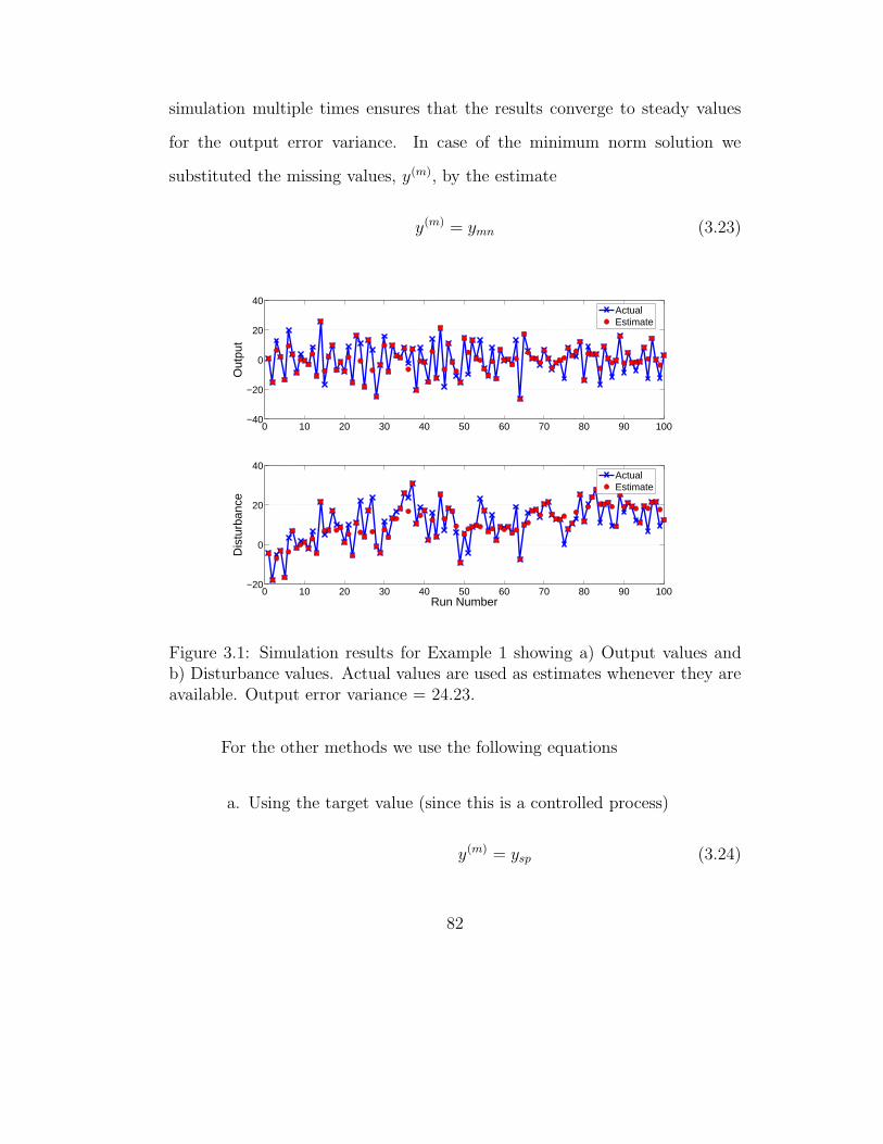
simulation multiple times ensures that the results converge to steady values

for the output error variance. In case of the minimum norm solution we

substituted the missing values, y(m), by the estimate

y(m) = ymn (3.23)

0 10 20 30 40 50 60 70 80 90 100−40

−20

0

20

40

Out

put

0 10 20 30 40 50 60 70 80 90 100−20

0

20

40

Run Number

Dis

turb

ance

ActualEstimate

ActualEstimate

Figure 3.1: Simulation results for Example 1 showing a) Output values andb) Disturbance values. Actual values are used as estimates whenever they areavailable. Output error variance = 24.23.

For the other methods we use the following equations

a. Using the target value (since this is a controlled process)

y(m) = ysp (3.24)

82

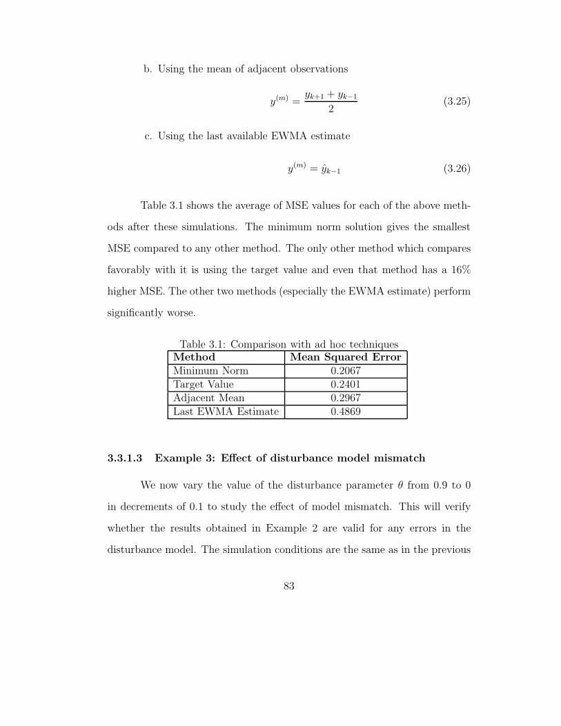
b. Using the mean of adjacent observations

y(m) =yk+1 + yk−1

2(3.25)

c. Using the last available EWMA estimate

y(m) = yk−1 (3.26)

Table 3.1 shows the average of MSE values for each of the above meth-

ods after these simulations. The minimum norm solution gives the smallest

MSE compared to any other method. The only other method which compares

favorably with it is using the target value and even that method has a 16%

higher MSE. The other two methods (especially the EWMA estimate) perform

significantly worse.

Table 3.1: Comparison with ad hoc techniquesMethod Mean Squared ErrorMinimum Norm 0.2067Target Value 0.2401Adjacent Mean 0.2967Last EWMA Estimate 0.4869

3.3.1.3 Example 3: Effect of disturbance model mismatch

We now vary the value of the disturbance parameter θ from 0.9 to 0

in decrements of 0.1 to study the effect of model mismatch. This will verify

whether the results obtained in Example 2 are valid for any errors in the

disturbance model. The simulation conditions are the same as in the previous

83

example. Figure 3.2 shows the change in MSE with change in the level of

mismatch. Since the value of θ is varied from 0.9 to 0, the value of λ required

changes from 0.1 to 1 [132]. Since we use a constant value of 0.3 for λ the

mismatch varies from 0.2 to -0.7.

−0.7 −0.6 −0.5 −0.4 −0.3 −0.2 −0.1 0 0.1 0.20.1

0.2

0.3

0.4

0.5

0.6

0.7

Mismatch in EWMA parameter

Mea

n S

quar

ed E

rror

Minimum NormAdjacent MeanTargetLast EWMA

Figure 3.2: Change in MSE with change in mismatch for EWMA parameterλ. The minimum norm solution produces the least MSE for lower values ofλ− θact but is outperformed at higher values by the adjacent mean method.

The plot clearly shows the superiority of the minimum norm solution

at positive mismatch. However, as the mismatch becomes negative, using

the adjacent mean is seen to outperform the minimum norm. Neither of the

remaining two methods have MSE values as low as the first two methods.

However, using the target value shows a minimum in the no mismatch case

(θ=0.7), which is expected. From a control standpoint, a positive mismatch

84

implies higher control effort than required, while a negative mismatch implies

less control effort. Thus, while it is seen that the minimum norm and target

methods are better for over-control than under-control, the adjacent mean and

EWMA methods perform worse under over-control conditions.

3.3.1.4 Example 4: Effect of sampling rate

We vary the sampling rate from 10% to 95% in increments of 5% to

observe any changes in MSE between the different methods under comparison.

The same simulation conditions are used as in Examples 2 and 3. Because the

sampling rate increases from 10% to 95%, we remove 90% to 5%, respectively,

of the values for each simulation accordingly. Figure 3.3 shows the change

in MSE with sampling rate. It is seen that the minimum norm solution is

always better at any sampling rate. In fact it outperforms using the mean and

EWMA estimate by 100% or more below sampling rates of 40%. Only using

the target is close to the minimum norm solution, but it never outperforms it

at any sampling rate.

3.3.1.5 Example 5: Effect of gain mismatch

We vary the value of δ used in Equation (3.5) from 0.5 to 2 in increments

of 0.1, using the same simulation conditions and a sampling rate of 75%. A

lower δ value implies that a lower gain is required while δ > 1 implies that

a higher gain is required. The results in Figure 3.4 show that the minimum

norm solution produces the lowest MSE at any gain mismatch.

85

In theory, the minimum norm solution should outperform each of the

other three methods irrespective of the sampling rate or the level of gain or

disturbance model mismatch. Since the adjacent mean and EWMA estimate

method have been proved inadequate, we will no longer use these two methods

for comparison. Only the minimum norm and set-point method will be used

in the following section. They will be referred to as the MN and SP methods

respectively.

0 10 20 30 40 50 60 70 80 90 1000

0.5

1

1.5

2

2.5

3

Sampling Rate

Mea

n S

quar

ed E

rror


Figure 3.3: Change in MSE with change in sampling rate. The minimumnorm solution produces the least MSE at all sampling rates. The MSE athigher sampling rates is comparable between all methods but deviates by alarge amount at lower sampling rates with the exception of the target valuemethod.

86

3.4 Kalman filter solution

3.4.1 State-space representation

The control system described in Equations (3.1) to (3.6) can be repre-

sented by state-space equations for a linear time-invariant model as follows:

xk+1 = Axk + βk (3.27)

with the transition matrix

A =

[1 0λ 1 − λ

](3.28)

0.5 1 1.5 20

0.4

0.8

1.2

1.6

2

δ

Mea

n S

quar

ed E

rror


Figure 3.4: Change in MSE with gain mismatch. The minimum norm solutionproduces the least MSE at any value of δ.

87

The process output consists of linear combinations of the state variables

corrupted by additive white noise and is given by

yk = Cxk + vk (3.29)

with

C =[1 −δ] (3.30)

In Equation (3.27) the state consists of actual and predicted distur-

bances used during the process run. This a non-classical way of representing

a controlled process but it aids in reconstructing the process output. Thus,

x ≡[ee

](3.31)

Also we use the following representations

βk =

[∆ek|k−1

0

](3.32)

yk = yactual − δysp (3.33)

where βk and vk are assumed to be independent noise sequences with covari-

ance matrix Σb and variance σ2v respectively. The measurement noise vk is

assumed to be negligible and therefore only nominal values are used for its

variance.

3.4.2 Kalman filter algorithm

We define the finite sample optimal estimate of the state vector xk+1

based on past outputs as

xk+1|k = E[xk+1|yk, . . . , y1] (3.34)

88

with

Vk+1|k = E[(xk+1 − xk+1|k)(xk+1 − xk+1|k)T ] (3.35)

as the error covariance matrix. Then the Kalman filter equations [19] can be

used to obtain the current estimate xk|k by recursive methods described in the

next section.

3.4.2.1 Forward Kalman filter

To run the recursive Kalman filter equations forward in time we start

with appropriate initial values x0 ≡ x0|0 and V0 ≡ V0|0. The optimal filtered

estimate is given by the recursive updating equation

xk|k = xk|k−1 +Kk(yk − Cxk|k−1) (3.36)

where the Kalman gain matrix Kk is given by

Kk = Vk|k−1CT (CVk|k−1C

T + σ2v)

−1 (3.37)

The prediction equations

xk|k−1 = Axk−1|k−1 (3.38)

and

Vk|k−1 = AVk−1|k−1AT + Σb (3.39)

use the updating equation of the error covariance matrix given by

Vk|k = (I −KkC)Vk|k−1 (3.40)

89

The finite sample innovation is expressed as

wk|k−1 = yk − Cxk|k−1 (3.41)

Equations (3.27) to (3.41) can be used to reconstruct a given time series of

outputs. In case of any missing values, the sample innovation wk|k−1 is taken

as zero, i.e., no change in the state estimate xk|k. As will be seen later, this

aspect can be improved upon.

3.4.2.2 Smoothed Kalman filter

To produce an expected value of xk conditioned on all N measurements

up to k, we use the Rauch-Tung-Striebel (R-T-S) fixed interval smoother [89]

which runs a Kalman filter forward followed by a fixed point smoother back-

wards. The equations are given as follows

yk|N = Cxk|N (3.42)

with

xk|N = xk|k + Vk|k−1AT

k Sk+1 (3.43)

where

Ak = A(I −KkC) (3.44)

and

Sk = AT

k Sk+1 + CT (CVk|k−1CT + σ2

v)−1wk|k−1 (3.45)

The Kalman gain matrix Kk is given by running the forward Kalman filter

(k = 1, . . . , N) while the equations are run backwards in time (k = N, . . . , 1).

90

The error covariance matrices are similarly obtained by the recursive

equations

Vk|N = Vk|k − Vk|k−1AT

k Tk+1AkVk|k−1 (3.46)

with

Tk = AT

k Tk+1Ak + CT (CVk|k−1CT + σ2

v)−1C (3.47)

The smoother is initialized with xN |N and VN |N produced by the forward

Kalman filter. Thus the data reconstruction occurs as follows. First the for-

ward Kalman filter is used to produce the Kalman gain and error covariance

matrices. When any measurement is missing, we use zero sample innovation

and proceed. This results in a complete set of gain and covariance matrices

which are now used while running the Kalman smoother backwards in time.

Estimates conditional to all measurements are now produced.

3.4.3 Using the minimum norm solution

We now use the datasets from the examples in the previous section and

carry out the same recursive calculations with one major difference; instead of

using a zero value of sample innovation for any missing measurement, we use

the minimum norm estimate from Equation (3.21) and substitute the latest

value of ∆e in Equation (3.32). Since the sample innovation has expected

value zero at any point but is unlikely to be zero, the minimum norm solution

is assumed to provide a better estimate. It also allows the covariance matrix

for the Kalman filter to evolve.

91

3.4.4 Simulations

3.4.4.1 Example 2 Revisited

To validate the Kalman filter approach combined with the minimum

norm solution, we perform the same simulation described in Example 2. Run-

ning the simulation multiple times ensures that the results converge on steady

values for the output mean squared error. The standard forward Kalman fil-

ter and smoothed Kalman filter methods are referred to as FKF and BKF

henceforth. When the minimum norm solutions are used they are referred

to as FKF-MN and BKF-MN respectively. Table 3.2 shows that using the

minimum norm solution is still better than any other method for white noise.

The FKF and BKF methods produce MSE values which are 50% higher than

the MN method. But when FKF-MN and BKF-MN are used, the MSE’s drop

considerably although they are still higher than the MN method.

Table 3.2: Comparison with previous techniquesMethod Mean Squared ErrorMN 0.2072SP 0.2429FKF 0.3649BKF 0.3021FKF-MN 0.2349BKF-MN 0.2573


We now vary the value of the disturbance parameter θ from 0.9 to 0 in

decrements of 0.1 as done earlier in Example 3. In Figure 3.5 it is seen that

92

the MN method still works well for low values of disturbance model mismatch.

However, at higher mismatch values the FKF-MN method produces lower

values of MSE. From a control standpoint, a positive mismatch implies higher

control effort than required, while a negative mismatch implies lower control

effort than required. Thus, while the MN and SP methods are better for over-

control than under-control, almost all the KF methods perform worse under

over-control conditions (with the exception of BKF-MN).

−0.7 −0.6 −0.5 −0.4 −0.3 −0.2 −0.1 0 0.1 0.20.1

0.2

0.3

0.4

0.5

0.6

0.7

0.8

0.9

Mismatch in EWMA parameter

Mea

n S

quar

ed E

rror

MNSPFKFBKFFKF−MNBKF−MN

Figure 3.5: Change in MSE with change in mismatch for EWMA parameterλ. MN method is best for lower mismatch values. Using the FKF-MN methodis best for higher mismatch.

93


We vary the sampling rate from 10% to 95% in increments of 5% to

observe any changes in MSE, as done before in Example 3. Figure 3.6 shows

that except for very high sampling rates, the MN method still produces the

lowest MSE in a simulated case. The MSE for all KF methods is significantly

higher than MN and SP for lower sampling rates. Interestingly, the MSE

for all KF methods drops rapidly once the threshold of 50% sampling rate is

crossed. This implies that KF methods may be inadequate at less than 50%

sampling rates. The figure also shows that if we know the tolerance for the

mean squared error, say 0.4, we can reduce our sampling rate from 100% to to

a lesser value, less than 55% in this case, by using the minimum norm solution.

The same tolerance requires higher sampling rates with the other methods.


We vary the value of δ used in Equation (3.5) from 0.5 to 2 in increments

of 0.1, similar to Example 5. Figure 3.7 shows that in case of gain mismatch,

the BKF and BKF-MN methods outperform the other methods when there is

significant error in the gain used. The FKF-MN is better than MN at higher

δ but is higher at lower δ. Based on simulation results, the FKF-MN method

is suitable in case of high δ and negative disturbance mismatch. For positive

disturbance mismatch MN method is preferable while BKF-MN dominates for

any gain mismatch.

94


We now consider three different manufacturing processes from the fab

in order to test our minimum norm solution. There are two etch processes and

one exposure process from which data were obtained from AMD.

0 5 10 15 20 25 30 35 40 45 50 55 60 65 70 75 80 85 90 95 1000

0.2

0.4

0.6

0.8

1

1.2

Sampling Rate

Mea

n S

quar

ed E

rror

LSSPFKFBKFFKF−LSBKF−LS

Figure 3.6: Change in MSE with change in sampling rate. The minimum normsolution produces the least MSE at all sampling rates. The MSE deviates bya large amount at lower sampling rates with the exception of the set-pointmethod. The error tolerance can be used to determine an acceptable samplingrate for the process.

The data from each of these processes is further sub-divided into threads

depending on the variation in products, tools and other factors. We will study

the effect of varying sampling rates on this data and see the impact on mean

squared error for the minimum norm solution as compared to other solutions.

The curves for sampling rates may not be as smooth as the ones seen in the

95

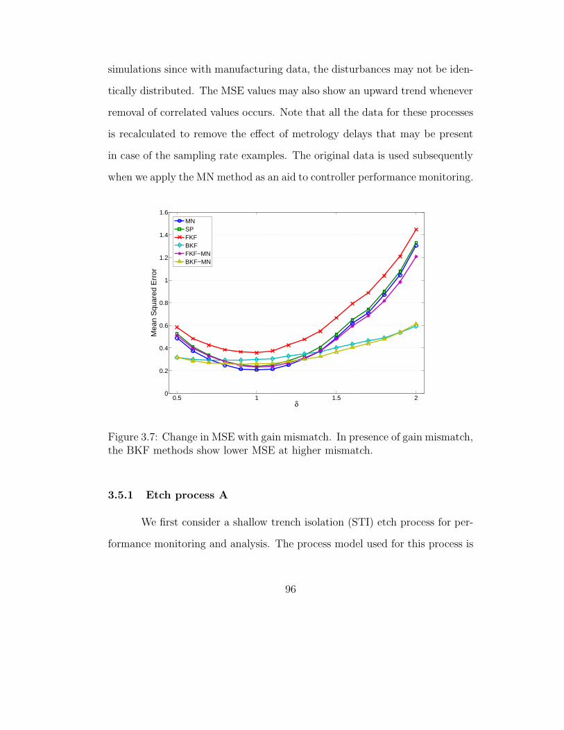
simulations since with manufacturing data, the disturbances may not be iden-

tically distributed. The MSE values may also show an upward trend whenever

removal of correlated values occurs. Note that all the data for these processes

is recalculated to remove the effect of metrology delays that may be present

in case of the sampling rate examples. The original data is used subsequently

when we apply the MN method as an aid to controller performance monitoring.

0.5 1 1.5 20

0.2

0.4

0.6

0.8

1

1.2

1.4

1.6

δ

Mea

n S

quar

ed E

rror


Figure 3.7: Change in MSE with gain mismatch. In presence of gain mismatch,the BKF methods show lower MSE at higher mismatch.

3.5.1 Etch process A

We first consider a shallow trench isolation (STI) etch process for per-

formance monitoring and analysis. The process model used for this process is

96

as follows

EtchDepth = EtchRate× EtchT ime+Bias (3.48)

The Bias is updated by EWMA as given in the previous sections. Accord-

ingly, the manipulated variable is EtchT ime, while the controlled variable is

EtchDepth. The data from this process is further segregated into 46 threads

with different settings for the EtchRate in each case.

3.5.1.1 Effect of sampling rate

Let us consider a single thread from the data and study the effect of

sampling rate on the error from each method discussed. The sampling rate is

varied from 10% to 95% in increments of 5. The data has 291 lots and the

missing data estimation is carried out on a run-to-run basis. The results are

shown in Figure (3.8). It is observed that the MN method is the best until

about 70% sampling rate, after which the SP and FKF-MN methods compete

well with it. The FKF method shows the highest MSE value at all sampling

rates. However, it may be safely concluded that the minimum norm solution

is the best method for the case of this dataset.

3.5.1.2 Cumulative study of all threads

We repeat the previous example for all 46 threads in etch process A

to compare the efficacy of each of the eight missing data estimation methods.

Each dataset is subjected to a sampling rate from 10% to 95% as before and

the method giving the lowest MSE is noted. We then calculate the fraction of

97

threads for which a particular method is the best for a given sampling rate.

0 10 20 30 40 50 60 70 80 90 1000

0.5

1

1.5

2

2.5

3

3.5

4

Sampling Rate

Mea

n S

quar

ed E

rror


Figure 3.8: Change in MSE with change in sampling rate for sample thread inetch process A. The minimum norm solution is seen to be the best at almost allsampling rates while the forward Kalman filter shows the worst performance.

The results are plotted in Figure (3.9). We observe that the MN method

is dominant at sampling rates below 50%. After that, the proportion of MN

decreases at the expense of FKF-MN and SP methods. The adjacent mean

method (represented henceforth as ADJ) and the FKF method also show good

results at very high sampling rates.

98

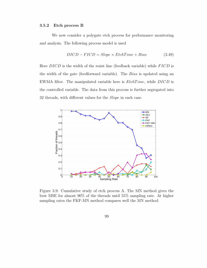
3.5.2 Etch process B

We now consider a polygate etch process for performance monitoring

and analysis. The following process model is used

DICD − FICD = Slope×EtchT ime+Bias (3.49)

Here DICD is the width of the resist line (feedback variable) while FICD is

the width of the gate (feedforward variable). The Bias is updated using an

EWMA filter. The manipulated variable here is EtchT ime, while DICD is

the controlled variable. The data from this process is further segregated into

32 threads, with different values for the Slope in each case.

0 10 20 30 40 50 60 70 80 90 1000

0.1

0.2

0.3

0.4

0.5

0.6

0.7

0.8

0.9

1

Sampling Rate

Fra

ctio

n of

thre

ads

MNADJSPFKFFKF−MNOthers

Figure 3.9: Cumulative study of etch process A. The MN method gives thebest MSE for almost 90% of the threads until 55% sampling rate. At highersampling rates the FKF-MN method compares well the MN method.

99


We now consider a single thread from the dataset for etch process A

to study the effect of varying sampling rate. This thread has 218 lots and the

sampling rates are varied as before from 10% to 95%.

0 10 20 30 40 50 60 70 80 90 1000

0.002

0.004

0.006

0.008

0.01

0.012

0.014

0.016

Sampling Rate

Mea

n S

quar

ed E

rror


Figure 3.10: Change in MSE with change in sampling rate for sample thread inetch process B. The MN method is significantly better at low sampling rates,while the FKF-MN method is the best at very high sampling rates. No othermethod shows a comparable performance.

The results seen in Figure (3.10) show that the MN method is sub-

stantially better at lower sampling rates. The other methods do well only

beyond a sampling rate of 75% with the FKF-MN method doing particularly

well. The SP method does not show a low MSE at any particular sampling

rate. Thus, we can again conclude that the MN method is the best for missing

100

data estimation for this dataset. It may be noted that overall, the magnitude

of MSE for all methods is fairly low compared to the thread selected in etch

process A.


We now conduct a similar experiment as the previous example for all

32 threads in this dataset and find the methods giving the best estimates.

With the sampling rate varied from 10% to 95% we note the best estimation

method at each rate based on MSE. We then calculate the fraction at each

sampling rate which corresponds to a particular method. The results plotted

in Figure (3.11) show that the MN method is the best up until 65% sampling

rate. Thereafter, the FKF and FKF-MN methods dominate. The BKF and

BKF-MN methods show some results at all sampling rates. It can also be seen

that as compared to etch process A, the MN method is not as dominant for

etch process B. In case of etch process A, the MN method fraction does not

fall below half till 80% sampling rate but in case of etch process B the same

happens as early as 65%.

3.5.3 Exposure process

We now consider a polygate exposure process for performance moni-

toring and analysis. The following process model is used

DICD = Slope× Exposure+Bias (3.50)

101

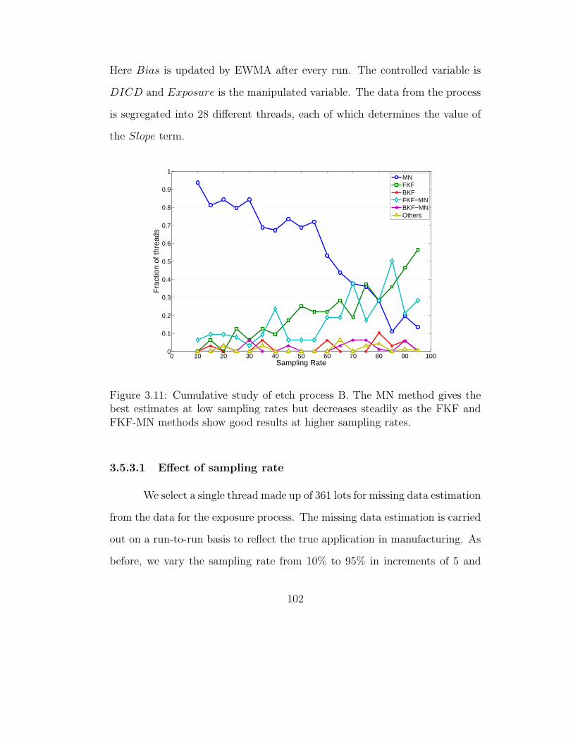
Here Bias is updated by EWMA after every run. The controlled variable is

DICD and Exposure is the manipulated variable. The data from the process

is segregated into 28 different threads, each of which determines the value of

the Slope term.

0 10 20 30 40 50 60 70 80 90 1000

0.1

0.2

0.3

0.4

0.5

0.6

0.7

0.8

0.9

1

Sampling Rate

Fra

ctio

n of

thre

ads

MNFKFBKFFKF−MNBKF−MNOthers

Figure 3.11: Cumulative study of etch process B. The MN method gives thebest estimates at low sampling rates but decreases steadily as the FKF andFKF-MN methods show good results at higher sampling rates.


We select a single thread made up of 361 lots for missing data estimation

from the data for the exposure process. The missing data estimation is carried

out on a run-to-run basis to reflect the true application in manufacturing. As

before, we vary the sampling rate from 10% to 95% in increments of 5 and

102

plot the results in Figure (3.12). It shows that the MN method is clearly the

best at almost all sampling rates. No other method is has a lower MSE and

FKF is particularly bad. Also, in this case the magnitude of MSE is closer to

that of the thread selected in etch process A.

0 10 20 30 40 50 60 70 80 90 1000

0.02

0.04

0.06

0.08

0.1

0.12

0.14

0.16

0.18

0.2

Sampling Rate

Mea

n S

quar

ed E

rror


Figure 3.12: Change in MSE with change in sampling rate for sample threadin exposure process. The MN method is clearly the best at all sampling rates.The other methods form best to worst are SP, BKF-MN, BKF, FKF-MN andFKF in that order.


We now study all 28 threads for the exposure process to determine the

best missing data estimation method at various sampling rates. The procedure

is as before with variation in sampling rates from 10% to 95% and the best

103

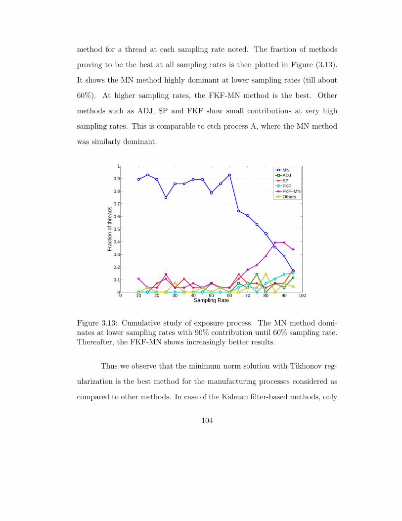
method for a thread at each sampling rate noted. The fraction of methods

proving to be the best at all sampling rates is then plotted in Figure (3.13).

It shows the MN method highly dominant at lower sampling rates (till about

60%). At higher sampling rates, the FKF-MN method is the best. Other

methods such as ADJ, SP and FKF show small contributions at very high

sampling rates. This is comparable to etch process A, where the MN method

was similarly dominant.

0 10 20 30 40 50 60 70 80 90 1000

0.1

0.2

0.3

0.4

0.5

0.6

0.7

0.8

0.9

1

Sampling Rate

Fra

ctio

n of

thre

ads

MNADJSPFKFFKF−MNOthers

Figure 3.13: Cumulative study of exposure process. The MN method domi-nates at lower sampling rates with 90% contribution until 60% sampling rate.Thereafter, the FKF-MN shows increasingly better results.

Thus we observe that the minimum norm solution with Tikhonov reg-

ularization is the best method for the manufacturing processes considered as

compared to other methods. In case of the Kalman filter-based methods, only

104

the forward Kalman filter-based methods and in particular the FKF-MN meth-

ods are found to be useful. The smoothed Kalman filter-based methods do not

have a significant impact on the estimation. This is mainly because in case of

manufacturing data we did the missing value estimation on a run-to-run basis

and not with the entire dataset. This reduces the utility of the these methods

to a large extent.

3.5.4 Application to data reconstruction for controller performancemonitoring

All the above examples for manufacturing data were based on planned

missingness, i.e., there is a uniformity in the missing values due to the use of

a sampling rate. But the original data from the fab contained some variable

delays as well, meaning that some EWMA estimates were calculated based on

only available values. This delay was mainly due to a backlog in the metrol-

ogy tool and adversely affects the controller performance monitoring technique

developed in Chapter 2 since it cannot incorporate variable metrology delays.

We therefore use the minimum norm solution optimized by Tikhonov regu-

larization to reconstruct values in this dataset whenever delays are present in

any current run. We then compare the performance index charts before and

after data reconstruction to see if there is an improvement in the performance

index. We exclude threads which show optimal performance since there can be

no more improvement in those. However, we find that for all three processes,

the average improvement over all threads considered is negligible. In some

case there is a marked improvement in the performance of the thread with the

105

variable delay accounted for. The following Figures (3.14) to (3.16) illustrate

these cases (DR = Data Reconstruction).

0 5 10 15 20 25 30 35 40 45 500.6

0.7

0.8

0.9

1

1.1

1.2

Calculation #

Per

form

ance

Inde

x

Before DRAfter DR

Figure 3.14: Improvement in performance with missing data estimation for athread from etch process A. The average delay is 1.1 in this case.

Thus using the missing data estimation method for data reconstruction

can lead to improvements in the performance of certain processes. The im-

provement is not guaranteed, however, and depends on the optimality of the

process itself. But it is certainly a good idea to remove the effects of variable

delay from a process before we calculate the performance index.

106


Several methods were developed and compared for estimation of missing

observations in a time-series from a run-to-run EWMA controlled process. The

minimum norm solution combined with Tikhonov regularization was compared

with simpler alternatives such as the mean of adjacent observations, using

the target value and the last EWMA estimate. Simulations show that the

minimum norm solution performs best in case of varying sampling rates and

gain mismatch. It was better for positive values of the disturbance model

parameter mismatch.

0 5 10 15 20 25 30 35 40 45 500.6

0.7

0.8

0.9

1

1.1

1.2

Calculation #

Per

form

ance

Inde

x

Before DRAfter DR

Figure 3.15: Improvement in performance with missing data estimation for athread from etch process A. The average delay is 1.4 in this case.

A state-space formulation was developed to reconstruct data affected by

107

missing values using the forward and smoothed Kalman filter. A combination

of minimum norm and Kalman filter was proposed as an improvement over the

smoothed Kalman filter, and the simulations were repeated. The simulations

showed the forward Kalman filter with minimum norm estimates performed

better for negative values of the disturbance parameter mismatch but the

minimum norm solution outperformed the Kalman filter methods for positive

values. In case of gain mismatch, the backward Kalman filter methods were

superior only for large mismatch in the gain. The minimum norm solution was

the best for gain mismatch values which are found in manufacturing.

0 5 10 15 20 25 30 35 40 45 500.4

0.5

0.6

0.7

0.8

0.9

1

Calculation #

Per

form

ance

Inde

x

Before DRAfter DR

Figure 3.16: Improvement in performance with missing data estimation for athread from etch process B. The average delay is 2.5 in this case.

In case of manufacturing data it was seen that the minimum norm so-

108

lution was dominant at low sampling rates, with other methods better only

at very high sampling rates. The method was successfully applied to man-

ufacturing data with variable delay which is to be analyzed for performance

monitoring purposes. The data reconstruction based on the minimum norm

solution was found to be useful in the case of some threads, which show an

improvement in the performance index trend over time. The results show that

the minimum norm and Kalman filter methods may be used in real-time to

produce forecasts for incoming batches in a run-to-run scenario. Since the

methods have been shown to reliable for most sampling rates, the measure-

ment of outputs in any process can be reduced to a large extent. This not only

reduces the processing time but also saves the cost of running the metrology

tool. We can also use them to filter measurements if the metrology tool is

noisy. The methods are also useful if post-process analysis is to be carried out

in a scenario where the EWMA controller has previously used out-of-sequence

data to control the input. In that case, the entire time-series can be recon-

structed for a longer horizon as if there were no sequencing issues. In the

future one may improve these methods by incorporating a Bayesian estima-

tion algorithm to improve the disturbance estimates, because an IMA (1,1)

disturbance sequence can be assumed to behave like a Markov chain under

some conditions.

109

Chapter 4

New State Estimation Methods for High-mix

Semiconductor Manufacturing Processes

4.1 Introduction

As run-to-run control has become more widely used throughout the

semiconductor industry, it has become apparent that some of its unique man-

ufacturing characteristics are driving the need for enhanced algorithm develop-

ment. One such trait is the high-mix of products made in a single factory, such

as an application specific integrated circuit (ASIC) fab. Not only might there

be a great many different products, but as industry requirements change and

technology advances, new products are introduced and old ones are phased

out. The mix of products is therefore constantly changing. Economic con-

ditions specific to the semiconductor industry are also a factor, because the

capital cost as a fraction of the revenue earned in the semiconductor industry

is higher than in other types of manufacturing industries. The high cost of

process equipment drives manufacturers to maximize the use of their tools,

having as little down or idle time as possible. In order to achieve this goal,

it is necessary to use whichever tool is available for processing in a given pro-

cess step, leaving little room for dedication of tools to specific product process

streams. Therefore, one lot of a specific product may take a very different

110

processing path through the fab than the next lot of that same product.

This problem has been addressed frequently only in recent years by

practitioners in the semiconductor industry. Miller [128] was the first to iden-

tify this problem and proposed four strategies for R2R control in high-mix

production: threads, grouping similar controllers, single global controllers and

information sharing controllers. Of these, the first two are very common in

practice but tend to require a large number of qualification runs. The global

controller is very rare and tends to be extremely process-specific. The infor-

mation sharing controller is much sought after, but applications for this type

are relatively recent in industry. Many results in literature are process spe-

cific, with photolithography being the most common process for application.

Conway et al. [35] describe a multi-level query-based application for overlay

control. Wan et al. [184] control lithography overlay using data sharing be-

tween a machine controller and a process induced error controller. Yue et

al. [193] used a context-based adaptive EWMA controller with an added in-

teraction term to control the exposure process. Levin et al. [105] focus on low

volume products for exposure and overlay control and add a bias term which

allows data from high volume products to be used. Park et al. [139] use neu-

ral networks for a lithography control system based on the stepper dynamics,

feedforward data, and the overlay bias.

Arnold et al. [147] consider R2R control of oxide CMP in a high-mix

environment by assigning polish rates depending on the tool being used. A

similar approach is used by Martinez [121] for STI CMP and by Neel et al. [133]

111

for STI etch. Chowdhury et al. [33] propose a gate etch controller which

consists of a master model whose bias is changed depending on the product.

Braun et al. [20] compare the performance of four control algorithms, namely,

threaded EWMA, context-based EWMA, adaptive EWMA and recursive least

squares. They find that the latter two do not provide a vast improvement

over the first two and also introduce additional parameters to be estimated.

Harrison et al. [69] compare threaded EWMA with context-based EWMA and

find that while the latter is better in case of high number of products, the

former is less sensitive to metrology delays. Zheng et al. [194] report an actual

manufacturing study where more than 70% of the products have less than ten

runs. They also find that tool-based control is unstable for non-stationary

disturbances while product-based control is sub-par for processes with large

drift.

Outside the semiconductor industry, the problem of decomposing time-

series into different sources has been studied very infrequently. This includes

work by Hillmer and Tiao [76] who decomposed ARIMA time-series into un-

observable seasonal, trend and noise components from partial fractions of the

variance expression. West [188] decomposes autoregressive time-series mod-

els into latent quasi-cyclical components using state-space models. This has

been extended to a general solution for time-series state space models with

time-invariant matrices by Godolphin and Johnson [53] and by Godolphin

and Triantafyllopoulos [54] for time-series with non-normal distributions.

112

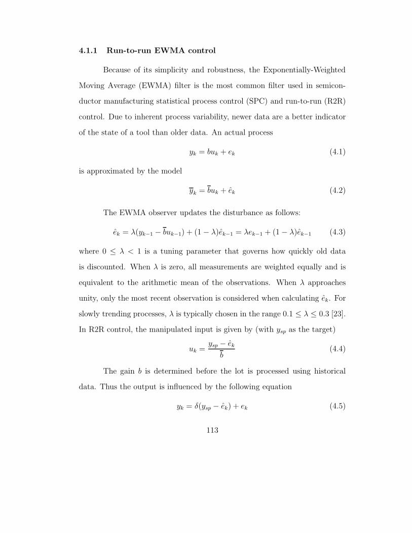
4.1.1 Run-to-run EWMA control

Because of its simplicity and robustness, the Exponentially-Weighted

Moving Average (EWMA) filter is the most common filter used in semicon-

ductor manufacturing statistical process control (SPC) and run-to-run (R2R)

control. Due to inherent process variability, newer data are a better indicator

of the state of a tool than older data. An actual process

yk = buk + ek (4.1)


yk = buk + ek (4.2)

The EWMA observer updates the disturbance as follows:

ek = λ(yk−1 − buk−1) + (1 − λ)ek−1 = λek−1 + (1 − λ)ek−1 (4.3)

where 0 ≤ λ < 1 is a tuning parameter that governs how quickly old data

is discounted. When λ is zero, all measurements are weighted equally and is

equivalent to the arithmetic mean of the observations. When λ approaches

unity, only the most recent observation is considered when calculating ek. For

slowly trending processes, λ is typically chosen in the range 0.1 ≤ λ ≤ 0.3 [23].

In R2R control, the manipulated input is given by (with ysp as the target)

uk =ysp − ek

b(4.4)

The gain b is determined before the lot is processed using historical

data. Thus the output is influenced by the following equation

yk = δ(ysp − ek) + ek (4.5)

113

where δ is the ratio of the actual gain to the gain used. In most cases this can

be safely assumed to be unity as the EWMA parameter λ can be adjusted to

compensate for gain mismatch.

One characteristic of the EWMA filter in Equation (4.3) is that it

provides the minimum mean squared error (MMSE) one step ahead forecast

for processes that follow an integrated moving average (IMA[1,1]) time series

model,

ek = ek−1 + ak − θak−1 (4.6)

where ak is a series of uncorrelated, zero mean, and normally distributed noise

and θ = 1 − λ [132]. Thus we assume that the process disturbance follows

the given model. The main objective in a run-to-run control application is the

accurate step-ahead forecast of this disturbance term, ek.

The organization of this chapter is as follows. In the next section we

explain previous methodologies in this area and their shortcomings. We also

define performance indices based on the accuracy of a given estimation method.

Then, a new state estimation method is proposed for the high-mix case. The

new method is based on a random walk model for the context states. More-

over, a moving window approach allows us to use a large amount of historical

data to produce better estimates for the context states. The estimation error

for this method for simulated processes is compared to threading and Just-in-

time Adaptive Disturbance Estimation (JADE). We also combine this random

walk approach with the recursive equations of the Kalman filter to produce

estimates and compare the performance of all methods with changing moving

114

window size for a simulated case. We also compare the decline in the esti-

mation performance index with increasing number of context items for each

method under consideration. Finally, we apply the method to an industrial

exposure process by extending the random walk model into an integrated mov-

ing average model, preserving the nature of the estimation at the expense of

a small but measurable error. In addition, we use weights to give prefer-

ence to the context that is more frequent and therefore more responsible for

variations. We then compare the random walk model-based method with its

Kalman filter-based counterpart and JADE.

4.2 Previous methodologies

The variations in product quality produced during manufacturing of-

ten are functions of the product being produced as well as the manufacturing

tools being used, which is termed manufacturing context. Different products

behave differently during processing due to factors such as differences in ma-

terials used, configuration or layout of devices and interconnects, feature size,

and overall chip size. To further complicate matters, seemingly identical tools

may process identical wafers differently based on such conditions as the number

of lots processed since the last maintenance event, small differences in tool con-

struction, or minor variations in ambient conditions. Different methods may

be employed to treat these variations. Feedforward control [161] measures the

incoming state of the lot in order to predict its impact on process performance.

Such a method requires an accurate measurement of the incoming state and a

115

predictive model. In addition, conventional application of feedforward control

requires 100% sampling of wafer lots, which is economically unfeasible for most

operations.

4.2.1 Threads

One method of wafer state estimation is to identify groups of lots that

have roughly the same incoming process state. Each group is segregated from

the rest of the groups based upon criteria that determine the incoming state.

These groups are referred to as control threads [12] or streamlines in the semi-

conductor industry. The ability to correctly identify control threads in a man-

ufacturing line requires determining which process factors affect the state of

the tool or incoming control state of a particular lot. For the most part, this

involves discrete context variables that apply to that lot, which includes pro-

cessing information such as the product or the layer at which the lot is run. In

addition, past context variables such as tools may also be applied in such cases

where they make a contribution to the state. The control threads methodol-

ogy lumps each of the states into a single, unique disturbance for the model.

Rather than compute an estimate of each state, the aggregate value of the

terms is instead calculated from the available process information. Thus,

yk = δ(ysp − ek) + eABC,k (4.7)

The combined process disturbance, eABC,k, represents a combination of three

sources of variation within the process, for example, product, layer and tool.

These three context variables would be the criteria (A,B,C) that were included

116

in the thread definition. By allowing only those lots with the same context

variable to update the estimate ek, the variance in the estimate is greatly

reduced. Vanli et al. [181] have proposed a rigorous statistical method to

identify the relevant context variables to include in the thread definition.

The inherent danger involving the use of threads is the potentially large

number of variables to be estimated, particularly in the case of high mix man-

ufacturing. Each criterion used to define a control thread divides the data set

by the number of values that criteria can take. With each additional parame-

ter in the thread definition, the control threads are again compartmentalized

as many times as there are possible values of the new criterion. Estimation

of the control state of each thread would then be based on fewer data points,

which would degrade control performance. Typically a fab has an uneven

mix of products, where there are a few products which have many lots and

many products of which only a few lots are run. These so-called low-runner

products present specific challenges to control systems. In high-mix fabs with

many products, some of the feedback loops may operate with long time pe-

riods between data points in the feedback loop. This long delay results in

a loss of information about the process tool contribution to the variance in

that specific product. The state of the process tool may experience drifts or

shifts during the time period in between low-runner product feedback loop

data points. These changes to the process tool state cannot be inferred by

the controller state until the next lot with the same context is run. At that

time, the controller sees the process tool state change as a disturbance to the

117

particular feedback loop that must be rejected. Each feedback loop must com-

prehend and reject this disturbance separately, because there is no sharing of

information between feedback loops.

In the last few years, non-threaded state estimation methods have

drawn considerable interest [52, 140, 186]. These methods share information

among different contexts. Assuming that the interaction among different in-

dividual states is linear, different algorithms such as linear regression and the

Kalman filter can be applied to identify the contributions from different vari-

ation sources. One of the chief difficulties in these methods is the unobserv-

ability in the context matrix which needs to be inverted at every step. Each

method utilizes a different approach to handling this problem and making the

system observable.

4.2.2 Just-in-time adaptive disturbance estimation (JADE)

The JADE algorithm [52] attributes the disturbance to the linear sum

of individual context states. A weighted recursive least squares estimation is

used to identify the contributions to variation from each individual context

item. Thus, the JADE control model is

yk = buk + etot,k (4.8)

The disturbance term, etot,k is defined as

etot,k =

m∑i

ei,k (4.9)

118

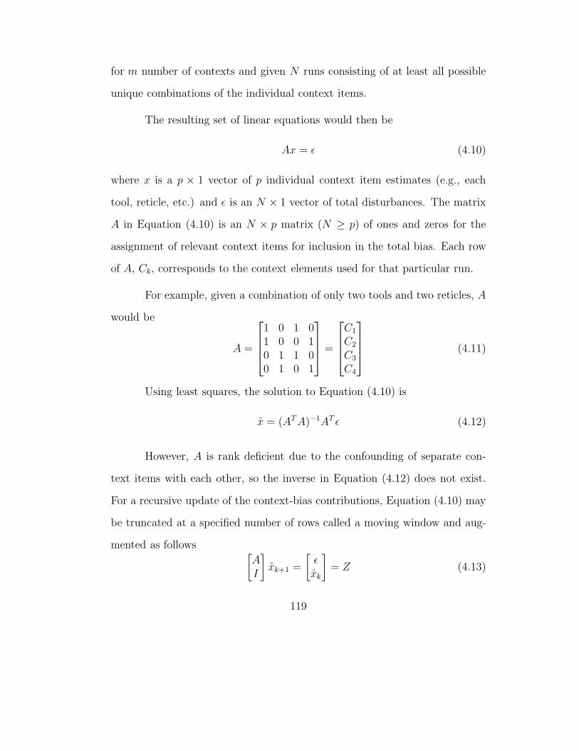
for m number of contexts and given N runs consisting of at least all possible

unique combinations of the individual context items.

The resulting set of linear equations would then be

Ax = ε (4.10)

where x is a p × 1 vector of p individual context item estimates (e.g., each

tool, reticle, etc.) and ε is an N × 1 vector of total disturbances. The matrix

A in Equation (4.10) is an N × p matrix (N ≥ p) of ones and zeros for the

assignment of relevant context items for inclusion in the total bias. Each row

of A, Ck, corresponds to the context elements used for that particular run.

For example, given a combination of only two tools and two reticles, A

would be

A =

⎡⎢⎢⎣

1 0 1 01 0 0 10 1 1 00 1 0 1

⎤⎥⎥⎦ =

⎡⎢⎢⎣C1

C2

C3

C4

⎤⎥⎥⎦ (4.11)

Using least squares, the solution to Equation (4.10) is

x = (ATA)−1AT ε (4.12)

However, A is rank deficient due to the confounding of separate con-

text items with each other, so the inverse in Equation (4.12) does not exist.

For a recursive update of the context-bias contributions, Equation (4.10) may

be truncated at a specified number of rows called a moving window and aug-

mented as follows [AI

]xk+1 =

[εxk

]= Z (4.13)

119

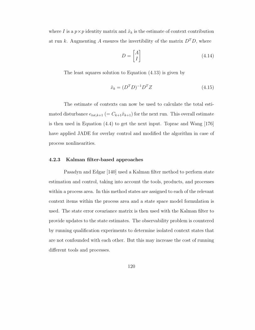
where I is a p×p identity matrix and xk is the estimate of context contribution

at run k. Augmenting A ensures the invertibility of the matrix DTD, where

D =

[AI

](4.14)

The least squares solution to Equation (4.13) is given by

xk = (DTD)−1DTZ (4.15)

The estimate of contexts can now be used to calculate the total esti-

mated disturbance etot,k+1 (= Ck+1xk+1) for the next run. This overall estimate

is then used in Equation (4.4) to get the next input. Toprac and Wang [176]

have applied JADE for overlay control and modified the algorithm in case of

process nonlinearities.

4.2.3 Kalman filter-based approaches

Pasadyn and Edgar [140] used a Kalman filter method to perform state

estimation and control, taking into account the tools, products, and processes

within a process area. In this method states are assigned to each of the relevant

context items within the process area and a state space model formulation is

used. The state error covariance matrix is then used with the Kalman filter to

provide updates to the state estimates. The observability problem is countered

by running qualification experiments to determine isolated context states that

are not confounded with each other. But this may increase the cost of running

different tools and processes.

120

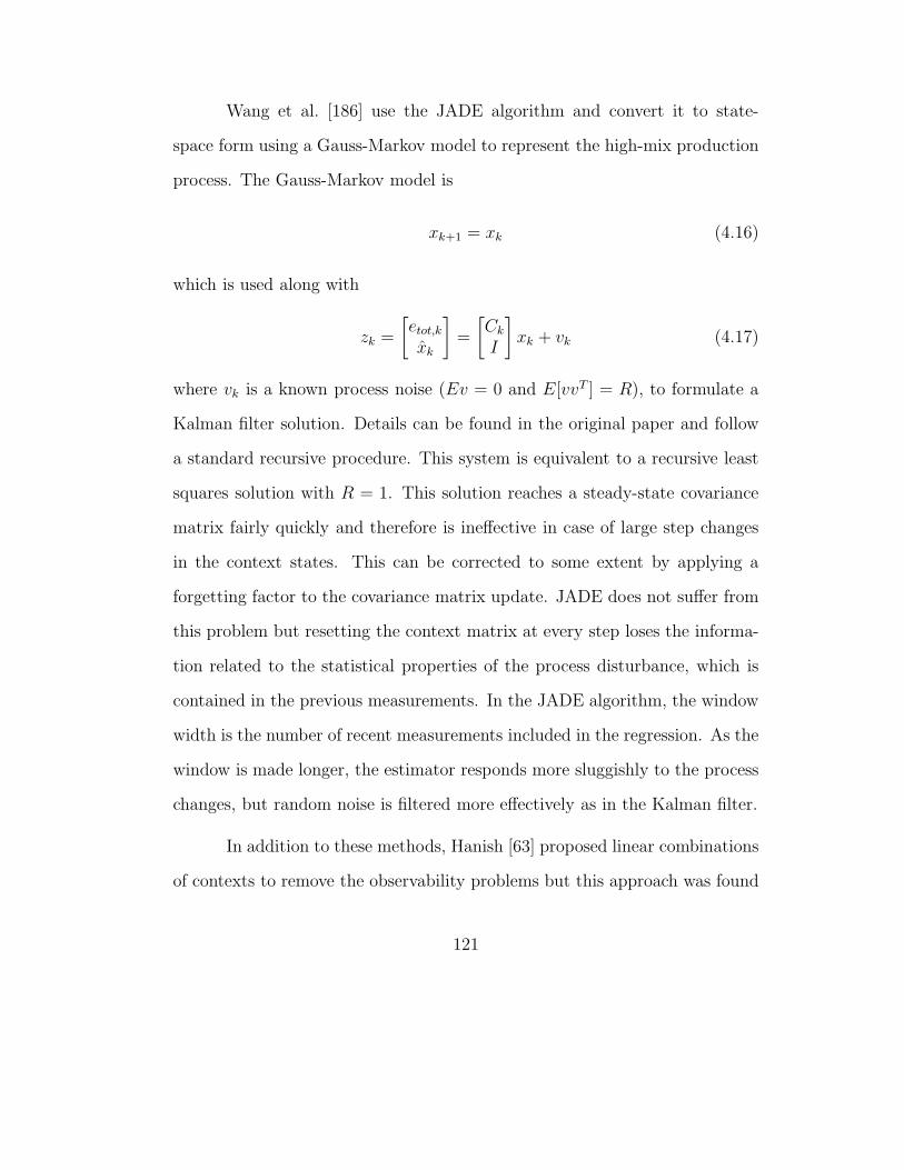
Wang et al. [186] use the JADE algorithm and convert it to state-

space form using a Gauss-Markov model to represent the high-mix production

process. The Gauss-Markov model is

xk+1 = xk (4.16)

which is used along with

zk =

[etot,k

xk

]=

[Ck

I

]xk + vk (4.17)

where vk is a known process noise (Ev = 0 and E[vvT ] = R), to formulate a

Kalman filter solution. Details can be found in the original paper and follow

a standard recursive procedure. This system is equivalent to a recursive least

squares solution with R = 1. This solution reaches a steady-state covariance

matrix fairly quickly and therefore is ineffective in case of large step changes

in the context states. This can be corrected to some extent by applying a

forgetting factor to the covariance matrix update. JADE does not suffer from

this problem but resetting the context matrix at every step loses the informa-

tion related to the statistical properties of the process disturbance, which is

contained in the previous measurements. In the JADE algorithm, the window

width is the number of recent measurements included in the regression. As the

window is made longer, the estimator responds more sluggishly to the process

changes, but random noise is filtered more effectively as in the Kalman filter.

In addition to these methods, Hanish [63] proposed linear combinations

of contexts to remove the observability problems but this approach was found

121

to be sub-optimal as compared to other methods [186]. Good and Schulze [57]

propose a singular value decomposition (SVD) approach to initialize thread

states.

4.2.4 Defining performance indices for estimation accuracy

We may define a performance index for any estimation procedure by

equating it with the correlation coefficient of the estimated process disturbance

with the actual process disturbance. Thus the estimation performance index

is given by

EPI = 1 − εT ε

εT ε(4.18)

where ε = ε− x is the estimation error vector at each estimation step and ε is

the total process disturbance vector at that step. EPI should be as close to

unity as possible for a good estimation technique, since that implies that the

process is relatively unaffected by estimation errors. A negative value indicates

that the estimation method is inappropriate for the given process.

4.3 New model-based algorithm

The earlier models for context states assume that the state is static as

in Equation (4.16) or that there is a known state error with diagonal covariance

matrix [186] given by

xk+1 = xk + wk (4.19)

with E[wwT ] = Q as the state covariance matrix. This prevents the error

covariance matrix from shrinking to zero over time, which is one of the prob-

122

lems with using a Kalman filter approach. But the assumption of a diagonal

covariance matrix implies that there is no correlation between the individual

context states. This assumption may not hold true in all cases. For example

some tool-product combination can have correlated states. Also, the states

may not remain static in any given set of data but could evolve over time,

with or without use. This leads us to propose a new model for context state

behavior, which is discussed in the next subsection.

4.3.1 Random walk model

Any moving window of data considered for forecasting the next state

may contain the same context item (for example, tool A) more than once.

But earlier methods of state estimation assume that the given context state

is unchanged within the given window of data. Here we assume that each

context state follows the model in Equation (4.19) with wk white noise vector

having zero mean and finite unknown covariance, thus making it a random

walk model. The total disturbance etot,k is also a random walk model due to

linearity. This is equivalent to an EWMA filter system with parameter λ = 1

(see Equation 4.6).

Now consider the simple case considered in Equation (4.11) with two

tools (a,b) and two reticles (R,S). Let there be six runs producing six distur-

bance measurements. We need to forecast the seventh disturbance which uses

tool a and reticle S. The sequence of runs is a−R, a−S, b−R, b−R, a−S, b−S

123

producing the context matrix A for JADE and related methods as

Ax =

⎡⎢⎢⎢⎢⎢⎢⎣

1 0 1 01 0 0 10 1 1 00 1 1 01 0 0 10 1 0 1

⎤⎥⎥⎥⎥⎥⎥⎦

⎡⎢⎢⎣abRS

⎤⎥⎥⎦ =

⎡⎢⎢⎢⎢⎢⎢⎣

e1e2e3e4e5e6

⎤⎥⎥⎥⎥⎥⎥⎦

= ε (4.20)

But if we consider a random walk model as in Equation (4.19) for each

context i, we have

xi,k+2 = xi,k+1 + wi,k+1 = xi,k + wi,k + wi,k+1 (4.21)

Thus each context state can be expressed as a linear combination of an

earlier state and all the white noise terms from the earlier state to the current

state. Thus for the example of six runs considered above, the context matrix

A now looks as follows

Ax = ε (4.22)

with

A =

⎡⎢⎢⎢⎢⎢⎢⎣

1 0 0 0 0 0 1 0 0 0 0 01 1 0 0 0 0 0 0 0 1 0 00 0 0 1 0 0 1 1 0 0 0 00 0 0 1 1 0 1 1 1 0 0 01 1 1 0 0 0 0 0 0 1 1 00 0 0 1 1 1 0 0 0 1 1 1

⎤⎥⎥⎥⎥⎥⎥⎦

(4.23)

and

x =[a α1 α2 b β1 β2 R γ1 γ2 S δ1 δ2

]T(4.24)

Here the α, β, γ, δ are the white noise disturbances corresponding to the con-

text states a, b, R, S respectively. Thus, it seems that by incorporating the

124

random walk model into the context matrix, we have increased the size of the

matrix. But it can be shown that while the context matrix in Equation (4.20)

is rank deficient, the one in Equation (4.23) is full rank. Thus, while the earlier

matrix requires augmenting to make an inverse possible (thus increasing the

size of the matrix in any case), the latter does not require any such manipula-

tion. In fact it can be shown that any such matrix derived from a random walk

model is always full rank (see Appendix C for proof). Such a general matrix

has size N ×mN , where N is the moving window size and m is the number of

contexts; while the augmented matrix in JADE has size (p+N) × p, where p

is the total number of context items. Thus in the example considered, we have

N = 6, m = 2 (tool and reticle) and p = 4 (a, b, R, S). Notice that the matrix

structure ensures that the number of row is always less than or equal to the

number of columns. Therefore to solve for x in Equation (4.22), we use the

right pseudo-inverse of A which minimizes the norm of x (see Appendix E).

Then the estimate is given by

x = AT (AAT )−1ε (4.25)

Thus, while for JADE the matrix to be inverted is ATA with size p× p, with

the random walk model, we invert the matrix AAT which has size N × N .

This means that the computational power required for JADE depends on the

total number of context items present in the system but with the random

walk model, we can control the computational power needed by adjusting the

moving window size.

125

The estimate for the seventh run (a−S) is then given by using the last

available estimates for both contexts. Thus,

e7 =[1 1 1 0 0 0 0 0 0 1 1 1

]x (4.26)

since each white noise sequence has expected value zero at any time.

4.3.2 Moving window approach

In a moving window approach we consider the last N runs of the pro-

cess, irrespective of whether all the contexts are present in those runs. If any

contexts that are to be used in the next run are not available in the moving

window, we just use the last available estimate for that context. The context

matrix evolves with time as the window moves, i.e., we recalculate A after ev-

ery run based on the latest N measurements and the contexts used in those. A

moving window thus ensures that the computational effort required is steady

over time and does not balloon up with more and more data. Also, the random

walk model allows us to consider all the latest measurements without having

to remove rows having identical context combinations (or threads) since the

row corresponding to the same threads has different elements. This is because

individual contexts within the thread evolve by the given model. The selection

of N however, is not simple since it demands a trade-off between maximizing

the use of available data and minimizing the computation time required to

invert A. For initial runs, the window size is limited by the available data.

Once we have enough data, we may restrict the matrix to a reasonable size

based on the computational power available.

126

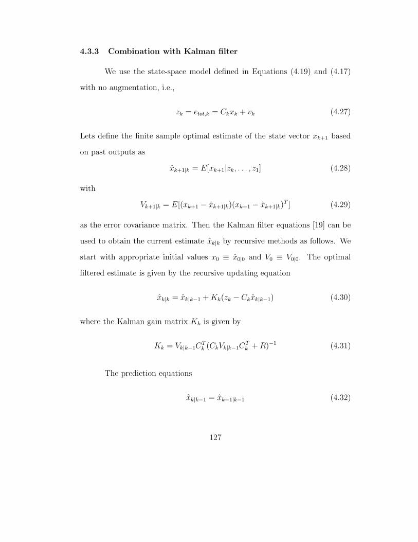
4.3.3 Combination with Kalman filter

We use the state-space model defined in Equations (4.19) and (4.17)

with no augmentation, i.e.,

zk = etot,k = Ckxk + vk (4.27)

Lets define the finite sample optimal estimate of the state vector xk+1 based

on past outputs as

xk+1|k = E[xk+1|zk, . . . , z1] (4.28)

with

Vk+1|k = E[(xk+1 − xk+1|k)(xk+1 − xk+1|k)T ] (4.29)

as the error covariance matrix. Then the Kalman filter equations [19] can be

used to obtain the current estimate xk|k by recursive methods as follows. We

start with appropriate initial values x0 ≡ x0|0 and V0 ≡ V0|0. The optimal

filtered estimate is given by the recursive updating equation

xk|k = xk|k−1 +Kk(zk − Ckxk|k−1) (4.30)

where the Kalman gain matrix Kk is given by

Kk = Vk|k−1CTk (CkVk|k−1C

Tk +R)−1 (4.31)

The prediction equations

xk|k−1 = xk−1|k−1 (4.32)

127

and

Vk|k−1 = Vk−1|k−1 +Q (4.33)

use the updating equation of the error covariance matrix given by

Vk|k = (I −KkCk)Vk|k−1 (4.34)

Now, we can use the estimates provided by the random walk model-

based solution of the moving window data to provide an estimate for the state

disturbance wk as

wk = xk,KF − xk,MN (4.35)

This can be used to update the covariance matrix Q = E[wwT ] for the next

run. Simulations have shown that this estimate is better than using a constant

diagonal Q matrix since this allows the error covariance matrix V to evolve

with time and not reach steady state.

4.4 Results from simulated data

To illustrate the characteristics of the non-threaded state estimation,

we consider the following a number of simple examples with multiple tools,

layers and products. Both step and ramp disturbances are included in the

individual states as they are frequently experienced in semiconductor manu-

facturing processes, and white noise is added to the final measurements. Note

that while the data series for each context remains the same, every time the

we simulate new output data based on context probabilities, a new output

128

series is created. Therefore the total output shown in the following figures

only represent a single simulation. The following processes are considered:

Process 1: The process context consist of three categories (tool, layer,

product), with two tools, two layers and three products. Simulation of the

process is carried out to generate a total of 500 runs as shown in Figure (4.1).

The context realization for each run is randomly selected based on a given

probability of occurrence for the available choices in each of the three categories

of the context. The running probability for each context is indicated in the

figure. A total of twelve threads are possible in this scenario. Of these, 4 are

high running while the rest are low running threads.

Process 2: Now we consider processes whose contexts follow a random

walk model. Consider that the process has two products, two layers and two

tools. Simulation of the process is carried out to generate a total of 500 runs

as shown in Figure (4.2). It also shows the probability of each context state

used. A total of eight threads are possible in this scenario. Of these, 3 are

high running while the rest are low running threads.

Process 3: Consider a very high mix process where the contexts follow

a random walk model as before. Consider that the process has five products,

five layers and five tools. Simulation of the process is carried out to generate

a total of 500 runs as shown in Figure (4.3). Table (4.1) shows the probability

of each context state used. A total of 125 threads are possible in this scenario.

All of these are low running threads.

129

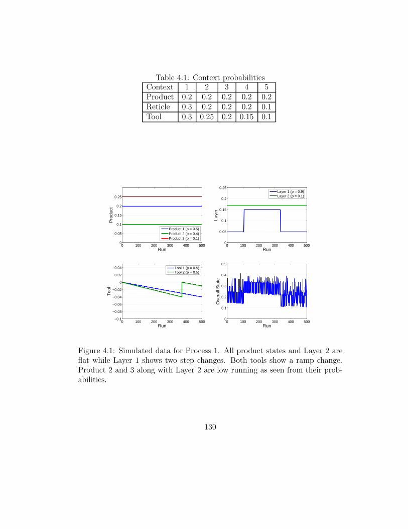
Table 4.1: Context probabilitiesContext 1 2 3 4 5Product 0.2 0.2 0.2 0.2 0.2Reticle 0.3 0.2 0.2 0.2 0.1Tool 0.3 0.25 0.2 0.15 0.1

0 100 200 300 400 5000

0.05

0.1

0.15

0.2

0.25

Run

Pro

duct

0 100 200 300 400 5000

0.05

0.1

0.15

0.2

0.25

Run

Laye

r

0 100 200 300 400 500−0.1

−0.08

−0.06

−0.04

−0.02

0

0.02

0.04

Run

Too

l

0 100 200 300 400 5000

0.1

0.2

0.3

0.4

0.5

Run

Ove

rall

Sta

te

Layer 1 (p = 0.9)Layer 2 (p = 0.1)

Product 1 (p = 0.5)Product 2 (p = 0.4)Product 3 (p = 0.1)

Tool 1 (p = 0.5)Tool 2 (p = 0.5)

Figure 4.1: Simulated data for Process 1. All product states and Layer 2 areflat while Layer 1 shows two step changes. Both tools show a ramp change.Product 2 and 3 along with Layer 2 are low running as seen from their prob-abilities.

130

These three processes are used to compare the estimates provided by

threads, JADE, random walk model and random walk-based Kalman filtering.

These are referred to as EWMA, JADE, RW and KF-RW henceforth.

0 100 200 300 400 500−1

−0.5

0

0.5

1

1.5S

tate

0 100 200 300 400 500−1

−0.5

0

0.5

1

1.5

Sta

te

0 100 200 300 400 500−1

−0.5

0

0.5

1

1.5

Run

Sta

te

0 100 200 300 400 500−1

−0.5

0

0.5

1

1.5

2

Run

Sta

te

Tool 1 (p = 0.9)Tool 2 (p = 0.1)

Product 1 (p = 0.2)Product 2 (p = 0.8)

Reticle 1 (p = 0.7)Reticle 2 (p = 0.3)

Figure 4.2: Simulated data for Process 2. Product 2 shows a ramp changewhile Tool 2 is variable. The remaining contexts are relatively flat. Product1, Reticle 2 and Tool 2 are low running.

In each case the data set is simulated ten times based on the probabil-

ities for the contexts. A pre-specified moving window is used to estimate the

next output using each of the five methods. Thus for each moving window

specified, we obtain ten values of the mean squared error. These are then

averaged to get a smoothed value for the mean squared error (MSE). In addi-

tion, each output dataset is normalized to zero mean and unit variance before

analysis but no initial values are provided, i.e., all states start with zero initial

131

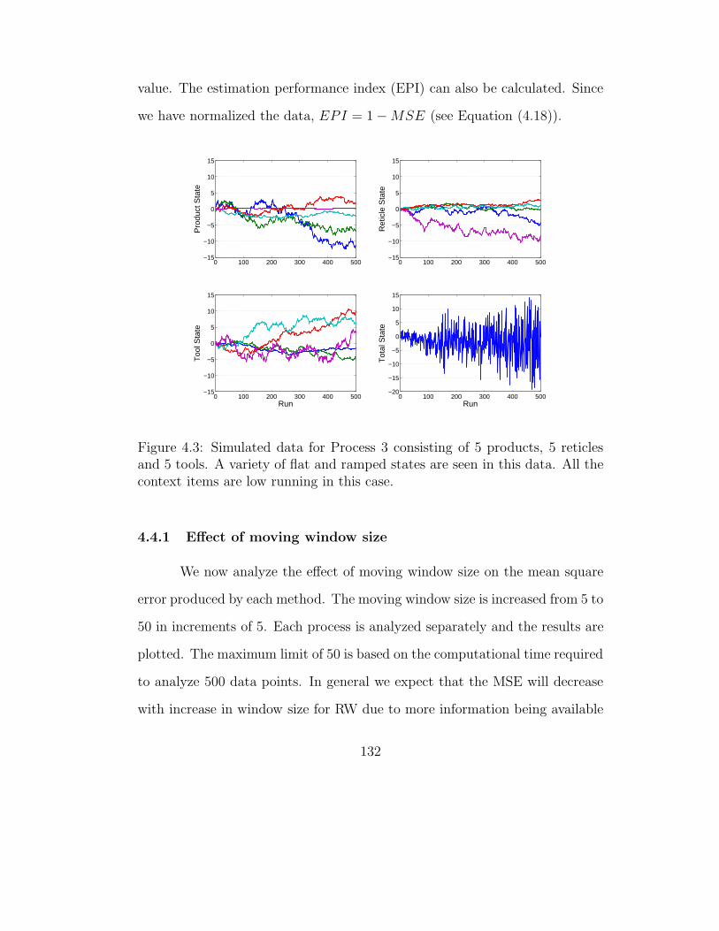
value. The estimation performance index (EPI) can also be calculated. Since

we have normalized the data, EPI = 1 −MSE (see Equation (4.18)).

0 100 200 300 400 500−15

−10

−5

0

5

10

15

Pro

duct

Sta

te

0 100 200 300 400 500−15

−10

−5

0

5

10

15

Ret

icle

Sta

te

0 100 200 300 400 500−15

−10

−5

0

5

10

15

Run

Too

l Sta

te

0 100 200 300 400 500−20

−15

−10

−5

0

5

10

15

Run

Tot

al S

tate

Figure 4.3: Simulated data for Process 3 consisting of 5 products, 5 reticlesand 5 tools. A variety of flat and ramped states are seen in this data. All thecontext items are low running in this case.

4.4.1 Effect of moving window size

We now analyze the effect of moving window size on the mean square

error produced by each method. The moving window size is increased from 5 to

50 in increments of 5. Each process is analyzed separately and the results are

plotted. The maximum limit of 50 is based on the computational time required

to analyze 500 data points. In general we expect that the MSE will decrease

with increase in window size for RW due to more information being available

132

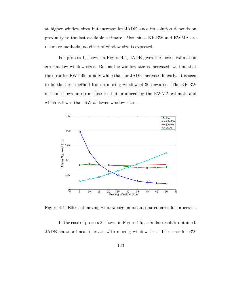
at higher window sizes but increase for JADE since its solution depends on

proximity to the last available estimate. Also, since KF-RW and EWMA are

recursive methods, no effect of window size is expected.

For process 1, shown in Figure 4.4, JADE gives the lowest estimation

error at low window sizes. But as the window size is increased, we find that

the error for RW falls rapidly while that for JADE increases linearly. It is seen

to be the best method from a moving window of 30 onwards. The KF-RW

method shows an error close to that produced by the EWMA estimate and

which is lower than RW at lower window sizes.

0 5 10 15 20 25 30 35 40 45 50 550

0.05

0.1

0.15

0.2

0.25

Moving Window Size

Mea

n S

quar

ed E

rror

RWKF−RWEWMAJADE

Figure 4.4: Effect of moving window size on mean squared error for process 1.

In the case of process 2, shown in Figure 4.5, a similar result is obtained.

JADE shows a linear increase with moving window size. The error for RW

133

falls rapidly with increasing window size and betters the KF-RW, EWMA and

JADE methods after size 20. The KF-RW method again shows a result similar

to the EWMA estimates, indicating that it does not offer much advantage over

EWMA for both process 1 and process 2.

0 5 10 15 20 25 30 35 40 45 50 550

0.05

0.1

0.15

0.2

0.25

Moving Window Size

Mea

n S

quar

ed E

rror

RWKF−RWEWMAJADE


For process 3, shown in Figure 4.6, we see that the EWMA threading

method gives a high value of MSE at all window sizes. This is expected be-

cause as the number of threads increases, in this case to 125, the amount of

information contained in each thread decreases. As a result, the estimation

performance suffers. In the case of KF-RW, it is still better at lower window

sizes; JADE is better at most lower sizes but RW is the best at higher win-

dow size. Also, RW has the advantage that the moving window size may be

134

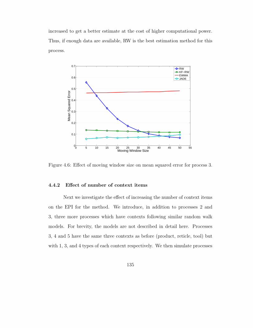
increased to get a better estimate at the cost of higher computational power.

Thus, if enough data are available, RW is the best estimation method for this

process.

0 5 10 15 20 25 30 35 40 45 50 550

0.1

0.2

0.3

0.4

0.5

0.6

0.7

Moving Window Size

Mea

n S

quar

ed E

rror

RWKF−RWEWMAJADE


4.4.2 Effect of number of context items

Next we investigate the effect of increasing the number of context items

on the EPI for the method. We introduce, in addition to processes 2 and

3, three more processes which have contexts following similar random walk

models. For brevity, the models are not described in detail here. Processes

3, 4 and 5 have the same three contexts as before (product, reticle, tool) but

with 1, 3, and 4 types of each context respectively. We then simulate processes

135

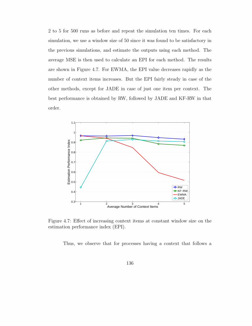
2 to 5 for 500 runs as before and repeat the simulation ten times. For each

simulation, we use a window size of 50 since it was found to be satisfactory in

the previous simulations, and estimate the outputs using each method. The

average MSE is then used to calculate an EPI for each method. The results

are shown in Figure 4.7. For EWMA, the EPI value decreases rapidly as the

number of context items increases. But the EPI fairly steady in case of the

other methods, except for JADE in case of just one item per context. The

best performance is obtained by RW, followed by JADE and KF-RW in that

order.

1 2 3 4 50.3

0.4

0.5

0.6

0.7

0.8

0.9

1

1.1

Average Number of Context Items

Est

imat

ion

Per

form

ance

Inde

x

RWKF−RWEWMAJADE

Figure 4.7: Effect of increasing context items at constant window size on theestimation performance index (EPI).

Thus, we observe that for processes having a context that follows a

136

random walk model, we can always find a window size for the data that gives

the lowest MSE using the RW method. The RW method is also least affected

by increasing context items in case of such processes. JADE is still competitive

in this regard, but suffers form not being able to give better results with more

data. The EWMA method is still good for small number of threads, but

rapidly loses its advantage as the number of context items increase, since the

number of threads increases in geometric proportion. The KF-RW method

does not suffer this drawback and gives a similar range of results irrespective

of the number of context items. But it is still inferior to the RW and JADE

methods.


We now consider high mix data for an exposure process from TI1. There

are two contexts, machine and reticle in this dataset consisting of 1713 points.

However, there are 4 machines and 80 reticles, which in combination produce

166 unique threads. As a result, most of the threads are low running even

though all the potential machine-reticle combinations (320) are not exhausted.

Figure 4.8 shows the number of threads versus number of runs. It is seen

that 90% of threads have fewer than 25 runs. As a result, we do not consider

threading (EWMA) as a method for comparison, there are not enough data per

thread to provide decent estimates without using some kind of initialization.

If the threads are initialized, the EWMA method has an unfair advantage due

1Texas Instruments, Inc.

137

to less than 20 points needing to be estimated in most cases.

4.5.1 Model adjustment based on process knowledge

Until now, we have assumed a random walk model for the process con-

texts in the absence of information to the contrary. But in the case of this

manufacturing data example, it is known that while the reticle states are static,

the machine states use an EWMA parameter λ = 0.4 during processing. This

implies that the machine states follow an integrated moving average model

of first order with parameter θ = 0.6. Recall that the random walk model

is a special case of an IMA model with θ = 0. We now use a random walk

model to describe the reticle state but use an IMA(1,1) model for the machine

state. Using an IMA(1,1) model changes the elements of A described in Equa-

tion (4.22). Consider the evolution of states according to this model analogous

to Equation (4.21)

xi,k+2 = xi,k+1 + wi,k+2 − θwi,k+1 = xi,k + wi,k+1 − θwi,k + wi,k+2 − θwi,k+1

= xi,k + (1 − θ)wi,k+1 + wi,k+2 − θwi,k

(4.36)

By neglecting the last term on the right hand side of Equation (4.36),

an evolving context matrix results consisting of not just ones and zeros as in

the random walk case, but also terms such as (1− θ) appearing in the interior

of the context matrix. Consider consecutive runs of a particular context. The

138

context sub-matrix then is as follows

Ai =

⎡⎢⎢⎢⎢⎢⎢⎢⎣

1 0 0 0 0 01 1 0 0 0 01 (1 − θ) 1 0 0 01 (1 − θ) (1 − θ) 1 0 0...

. . .. . .

...1 (1 − θ) . . . . . . (1 − θ) 1

⎤⎥⎥⎥⎥⎥⎥⎥⎦

(4.37)

0 10 20 30 40 50 60 70 80 90 1000

5

10

15

20

25

30

35

Number of runs

Num

ber

of th

read

s

Figure 4.8: Number of threads with specified number of runs. Most threadsare low-running with 10 high runners (> 35 runs).

Note that by neglecting the last term in Equation (4.36), we have pre-

served the structure of the context matrix, but at the same time an error is

introduced in the estimation. For the first run, there is no error. Then for the

second run, again there is no error, since the additional terms get incorporated

into the white noise estimate (wi,k+1 − θwi,k). But thereafter, we apply the

139

weight (1 − θ) to (wi,k+1 − θwi,k) instead of applying it to only wi,k+1. This

produces an error equivalent to θ2wi,k and in general, a constant error of zero

mean and variance θ4σ2w in the estimation. Because θ is always less than unity

and the white noise variance is considered small for an individual context, this

error is usually negligible.

4.5.2 Addition of context weights

So far we have not weighted the individual context states relative to

each other, since the number of context items is same for all contexts. But in

this manufacturing data case, we have a disproportionate effect of one context

(reticle) relative to the other (machine). As a result, we may need to consider

the fact that reticle states will change more rapidly over a given process window

than the machine states. Thus, more weight needs to be given to the context

sub-matrix corresponding to the reticles. To test this assertion, we now apply

weights to the context matrix A with certain conditions. If qM and qR are the

weights on the machine context and reticle context respectively,

AQ =[qRAR qMAM

](4.38)

where qM + qR = 1, while AM and AR are the sub-matrices corresponding to

the machine and reticle context. We now substitute this AQ in Equation (4.25)

in place of A to estimate the states.

To observe the impact of different weights we change qM from 0.1 to 0.9

and observe the effect on the mean squared error of the estimates. Also, the

140

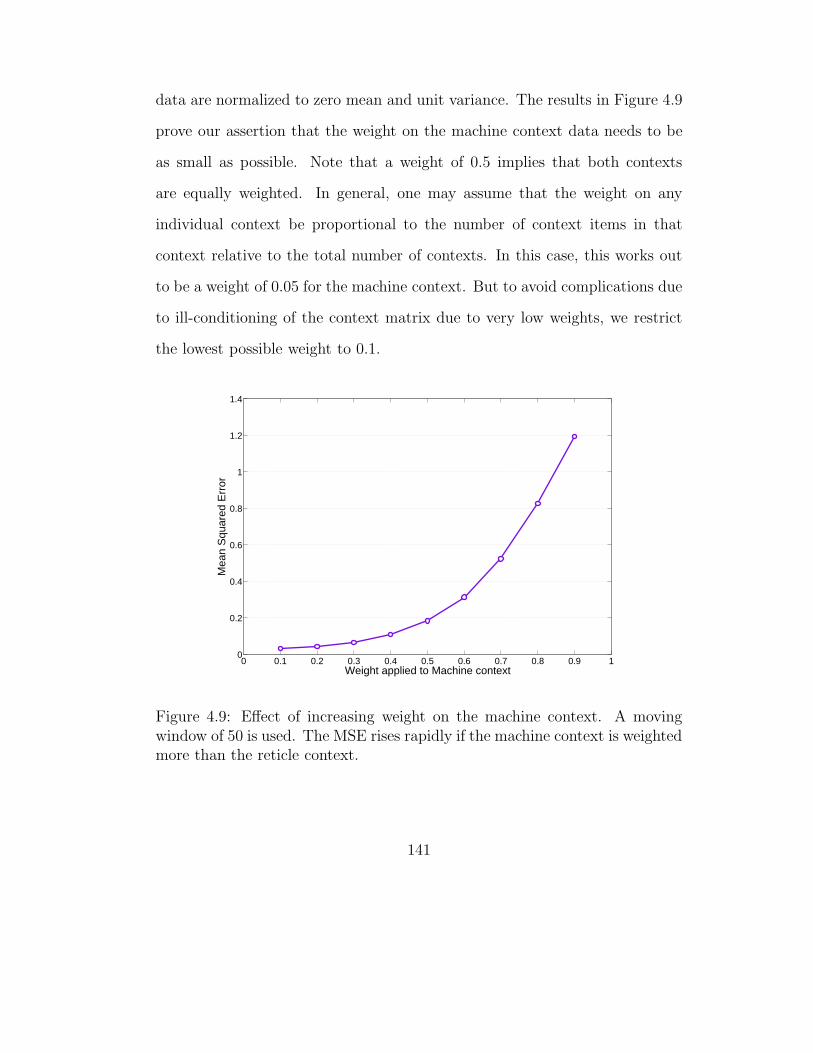
data are normalized to zero mean and unit variance. The results in Figure 4.9

prove our assertion that the weight on the machine context data needs to be

as small as possible. Note that a weight of 0.5 implies that both contexts

are equally weighted. In general, one may assume that the weight on any

individual context be proportional to the number of context items in that

context relative to the total number of contexts. In this case, this works out

to be a weight of 0.05 for the machine context. But to avoid complications due

to ill-conditioning of the context matrix due to very low weights, we restrict

the lowest possible weight to 0.1.

0 0.1 0.2 0.3 0.4 0.5 0.6 0.7 0.8 0.9 10

0.2

0.4

0.6

0.8

1

1.2

1.4

Weight applied to Machine context

Mea

n S

quar

ed E

rror

Figure 4.9: Effect of increasing weight on the machine context. A movingwindow of 50 is used. The MSE rises rapidly if the machine context is weightedmore than the reticle context.

141

4.5.3 Effect of moving window size

As with the simulated data, we consider what effect the moving win-

dow size has on the estimation error produced by the three methods under

consideration. They are henceforth referred to as IMA(RW), KF-IMA(RW)

and JADE. The estimation is carried out for moving window sizes ranging

from 5 to 50, in increments of 5. Also, the data are normalized to zero mean

and unit variance. The optimal weight of 0.1 determined previously for the

machine context is used. In case of JADE, the selection of weights follows the

procedure outlined in [52]. The results are shown in Figure 4.10.

0 5 10 15 20 25 30 35 40 45 50 550

0.01

0.02

0.03

0.04

0.05

0.06

0.07

0.08

0.09

0.1

Moving Window Size

Mea

n S

quar

ed E

rror

IMA(RW)KF−IMA(RW)JADE

Figure 4.10: Effect of moving window size on the estimation error. A weightof 0.1 is used on the machine context. The IMA(1,1) model-based estimationis seen to be the best method at all window sizes. The KF-IMA(RW) methodhas an unusually high MSE at window size 5, and is therefore off the scale.

142

The IMA(RW) method shows the lowest MSE for all window sizes.

Also, it shows a small decrease in MSE with increasing window size, as does

JADE. The KF-IMA(RW) method shows varying MSE with window size, but

on average the MSE is higher for this method than JADE and IMA(RW).

Thus, given the combination of the IMA(1,1) model and the weights applied

to individual contexts, the IMA (RW) method is seen to be the best estimator

for the given data.

We also plot the progression of error variance with each of these three

methods in Figure 4.11 for a window size of 50. As expected, after an initial

period of turbulence, the error variance declines gradually thereafter. But it

is observed that the KF-IMA(RW) method shows much lower error variance

initially than the other two methods (less than half). This continues until

about lot 500. After this, the method shows a slower decline than the other

two in terms of the error variance. Thus, we can claim that the KF-IMA(RW)

method is better in the initial period of data collection compared to JADE

and IMA(RW).


We have proposed a new method for state estimation in high-mix man-

ufacturing based on a random walk model for the context states. Moreover,

a moving window approach allows us to use a large amount of historical data

to produce better estimates for the context states. The results show that with

enough data available, this method produces the lowest estimation error for

143

simulated processes as compared to threading and JADE. We also combined

this random walk approach with the recursive equations of the Kalman filter

to produce estimates, which was found to be useful at lower window sizes.

In case of the individual contexts, it is found that with increasing number of

items per context, the random walk model is the most robust as it produces the

smallest decline in the estimation performance index. The greatest reduction

in performance is seen for the threading method and it is not recommended

for high mix systems.

200 400 600 800 1000 1200 1400 16000

0.1

0.2

0.3

0.4

0.5

0.6

0.7

0.8

0.9

1

Lot Number

Cum

ulat

ive

Err

or V

aria

nce

IMA(RW)JADEKF−IMA(RW)

Figure 4.11: Progression of error variance for all three methods under consid-eration for a moving window of 50. The KF-IMA(RW) method shows verylow error in the initial stages as compared to JADE and IMA(RW).

Thus, depending on the process, one can use either the random walk

model, or the random walk estimate-based Kalman filter method, or JADE.

144

We also applied the method to an industrial exposure process by extending

the random walk model into an integrated moving average model, preserving

the nature of the estimation at the expense of a small but measurable error.

In addition, we used weights to give preference to the context that was more

frequent and therefore more responsible for variations. As a result, we found

that the IMA(1,1) model gave the best estimate for the given data irrespec-

tive of the process window considered. In the future, one could compare this

method to a method based on Bayesian statistics [186], where the Kalman

filter covariance matrix is reset whenever a step disturbance occurs.

145

Chapter 5

Identification and Monitoring of PID

controlled Nonlinear Processes

5.1 Introduction

All processes are nonlinear but are approximated as linear models

through either linearization of the nonlinear terms or by neglecting the non-

linearity as long as the impact is minimal in the region of operation. As a

result, most controllers tend to be optimized only for the linear model under

consideration. This can result in sub-optimal performance if the linearized

operating region is very narrow since in that case, the impact of the nonlin-

ear contribution of the model has to be minimized by the original controller

settings. Even if the controller does not act directly on the nonlinear term,

it may influence it indirectly through the input. This is assuming that any

nonlinearity in the system can be expressed in terms of the input and/or out-

puts. In recent years, there has been a lot of focus on the identification and

control of nonlinear systems, especially with rapid advances in computational

capabilities. In the chemical processing industry, nonlinear behavior of plant

models is typically found for certain reactions such as polymerization and for

pH control. In the semiconductor manufacturing industry, typical examples

include furnaces, chemical mechanical planarization and dose-focus control.

146

5.1.1 Types of nonlinear models

A broad classification of nonlinear processes can be made in terms of

the nature of the nonlinearity, i.e. whether it is present in the manipulated

variable or the controlled variable [169]. When the manipulated variable or the

input is a static nonlinearity preceding a linear dynamical system, the model is

known as a Hammerstein model. An example of such a system is a linear plant

with nonlinear control valve characteristics. When the controlled variable or

output is a static nonlinear function following a linear dynamic plant, the

model is known as a Wiener model. Examples of such models include pH

control and distillation systems. In general, however, it is better to classify

systems according to their structure so that their identification is easier. Haber

and Unbehauen [62] use such a classification for nonlinear system identification

as follows

1. Block-oriented models: These include simple and generalized Wiener and

Hammerstein models as well as combinations of the two. They can be

identified by separation of the output signal to subsystems attributable

to the parallel channels of different degrees of nonlinearity. The sub-

systems are generally characterized in terms of Volterra kernels. The

models can also be identified using frequency methods or from impulse

or step responses.

2. Cascade models: Cascade models have a static nonlinear term between

linear input and output terms. The structure can then be identified

147

using correlation analysis or frequency methods or from impulse or step

responses.

3. Linear models with signal dependent parameters: These models can usu-

ally be linearized for small excitations around all possible working points

and its parameters are functions of any measurable or computable signal.

Polynomial models are typically used to express these functions and the

parameters can be identified from normal operating data or from step

responses of multiple linear regions.

4. Linear-in-parameters models: In this type, the nonlinear model is as-

sumed to be difference equation linear in the parameters. The model

components are usually polynomial functions of the input and output

signals. These are identified using orthogonal least squares techniques

utilizing regression analysis methods such as stepwise regression and for-

ward/backward regression to minimize the model components.

We will deal mainly with the last two types, as these can be parameter-

ized easily in terms of polynomial models. Polynomial models are simple and

also allow for a number of orders and powers to be considered. This ensures

that a large number of possible models is explored during model selection. Two

of the most common methods to deal with nonlinearities have already been

mentioned, viz. block oriented Wiener and Hammerstein models, and poly-

nomial models, most of whom are described using Nonlinear Auto-Regressive

with eXogenous input (NARX) models. Non-parametric methods to deal with

148

such systems include dead-zone estimators, artificial neural networks (mainly

radial basis function networks), piecewise-linear estimators, sigmoid networks,

tree partitions and wavelet networks. The mathematical properties of most of

these non-parametric estimation functions are reviewed by Juditsky et al. [95].

5.1.2 Other methods dealing with nonlinear control

The literature in this field is vast and multi-disciplinary. Therefore, we

will only mention a few significant works related to the approach used in this

chapter. Baumann and Rugh [7] propose a family of linearizations around con-

stant operating points for single input, multi-output systems. The eigenvalues

of the linearized closed-loop system are placed at invariant values for all op-

erating points. Johansen [93] uses Tikhonov regularization (see Appendix D)

for identification of nonlinear models that are ill-posed or ill-conditioned. A

final prediction error (FPE) criterion is used to determine the regularization

parameter γ in this case. Del Castillo and Yeh [39] provide the optimized adap-

tive quality controller (OAQC) for run-to-run MIMO control in semiconductor

manufacturing. A family of possible Hammerstein models is assumed for the

given process and the multivariate recursive least squares algorithm is used

to obtain parameter estimates. This is followed by a nonlinear optimization

using a mixed penalty-barrier method.

Helbig et al. [72] define nonlinearity measures and their lower bounds

to determine stable and unstable operating points for nonlinear systems. The

approach is also useful for nonlinearity tests for model structure validation

149

and controller structure selection, particularly for linearized systems. Hernjak

and Doyle [75] use these nonlinearity measures to compare PID, IMC, DMC

(Dynamic Matrix Control) and NMPC (Nonlinear Model Predictive Control)

for a mildly nonlinear quadruple tank system and a nonlinear bioreactor. The

results indicated that for the tank system, all methods were suitable. PID

controllers were found to be unsuitable for the bioreactor. Performance mea-

sures based on the relative change in the integral square error (ISE) for open

and closed loop were used to compare the different control systems. Aguirre

et al. [3] studied the grey-box identification of NARX models and the map-

ping of static nonlinearities and eigenvalues of the linearized functions into

the model structure. The results are useful in obtaining models with more

physical meaning and with a predefined steady-state characteristic.

Lachman-Shalem et al. [103] use a combination of genetic programming

and NMPC to control the photolithography process in semiconductor manu-

facturing. The critical dimension (CD) and the alignment are controlled using

the exposure, focus, resist thickness, temperature and time. Grimble [61] has

applied generalized minimum variance control to multivariate systems with

known input nonlinearities in conjunction with feedforward control. Mhaskar

et al. [127] tune PID controllers by using the input trajectory prescribed by

a nonlinear controller derived for the process under consideration. The PID

tuning parameters are then optimized by an objective function that minimizes

the difference between the input-output trajectory for both controllers. The

method, however, requires that an additional nonlinear controller be designed

150

for the express purpose of optimizing the PID controller. But no recommen-

dations are given as to the preferred type of such a nonlinear controller.

In this chapter we derive a performance metric and optimal parameters

for PID controllers, when they are used to control nonlinear processes. First,

techniques to identify nonlinearity in a process are introduced, namely, the

high order moments method which checks for nonlinearity and non-gaussianity

of process data. Then we propose polynomial NARX models to represent a

nonlinear process with the added advantage that these can be parameterized.

These NARX models are then considered as linear-in-parameters models and

a performance monitoring technique used for MIMO processes is applied. The

application differs from the original in the final optimization step, due to the

lack of inversion methods available for generalized NARX models. Finally we

apply this performance monitoring and optimization technique to the simu-

lated EWMA control case used in Chapter 2 and a P/PI control case from

literature. This is followed by its application to certain scenarios in semicon-

ductor manufacturing where a nonlinear process is linearized based on operat-

ing region. We derive the optimal parameters for two such cases, one involving

exposure-focus control for lithography, and the other related to a BEOL etch

process.

5.2 Detecting nonlinearity using higher order statistics

Before any design of optimal controllers for a process that is suspected

to be nonlinear, it is important to determine whether the nonlinearity is signif-

151

icant or may be ignored for most operating conditions. Detection of nonlinear-

ity from time-series data of a process has been pursued in literature by Stack

and Doyle [169] and Choudhury et al. [32] using higher order statistical tools.

Classical signal processing tools such as the power spectrum utilize only the

first and second order moments of mean and variance, respectively. In case of

nonlinear signals, the third and fourth order moments and their frequency do-

main counterparts are seen to be useful. In this chapter, we will explore these

higher order moments using the approach followed by Choudhury et al. [32]

and the nonlinearity tests pioneered by Hinich [77] and Rao and Gabr [153].

Let us first define two important higher order statistical concepts needed to

obtain a test for nonlinearity.

5.2.1 Bispectrum and Bicoherence

The autocorrelation function of a stationary process, yt is defined by

Ryy(j) = E[y∗t yt+j ] (5.1)

The power spectrum is the Fourier transform of the autocorrelation sequence

given as

Pyy(f) =

∞∑j=−∞

Ryy(j)e−i2πfj (5.2)

where f denotes the frequency. This equivalent to

Pyy(f) = E[YfY∗f ] (5.3)

where Yf is the Fourier transform of yt

Yf =∞∑

t=−∞yte

−i2πft (5.4)

152

A sufficient condition for the existence of the power spectrum is that the

autocorrelation be absolutely summable. The power spectrum is real valued

and nonnegative, that is, Pyy(f) ≥ 0; if yt is real valued, then the power

spectrum is also symmetric, that is, Pyy(f) = Pyy(−f).

The first order cumulant of a time-series is the mean of the process,

while the second order cumulant is the autocovariance sequence. The third

order cumulant is defined as

C3y(j, k) = E[y∗t yt+jyt+k] (5.5)

These third order cumulants are also symmetric in their arguments, that is

C3y(j, k) = C3y(k, j) = C3y(−j, k − j) (5.6)

for a stationary real-valued process. The bispectrum is then defined as the

Fourier transform of C3y(j, k) as

S3y(f1, f2) =∞∑

j=−∞

∞∑k=−∞

C3y(j, k)e−i2πf1je−i2πf2k (5.7)

The bispectrum is a function of two frequencies and in contrast with the power

spectrum which is real valued and nonnegative, the bispectrum is complex

valued. It is also symmetric for a real valued process as expected, with

S3y(f1, f2) = S3y(f2, f1) = S3y(f1,−f1 − f2)

= S3y(−f1 − f2, f2) = S∗3y(−f1,−f2)

(5.8)

The bicoherence is then defined as a normalized form of the bispectrum

given by

bic3y(f1, f2) =S3y(f1, f2)√

Pyy(f1 + f2)Pyy(f1)Pyy(f2)(5.9)

153

5.2.2 Nonlinearity and non-gaussianity

We use the fact that any nonlinear process produces a non-gaussian

time series as a first condition towards determining nonlinearity of a time-

series. The assumption here is that non-skewness implies Gaussianity and

skewness implies non-gaussianity.

5.2.2.1 Non-gaussianity test

The basic idea for a test of non-gaussianity was developed by Hinich [77]

using the bispectrum. It uses the proof of zero third order cumulants for a

linear process to postulate that if the bispectrum of a process is not zero, then

the process is non-Gaussian. Thus, we have a hypothesis testing problem for

non-gaussianity:

H1 : the bispectrum of yt is nonzero

H0 : the bispectrum of yt is zero(5.10)

Assuming we have good estimates of the power spectrum, the sample

estimate of the squared bicoherence is given by

|bic3y(f1, f2)|2 =|S3y(f1, f2)|2

Pyy(f1 + f2)Pyy(f1)Pyy(f2)(5.11)

It is known that sample estimates of the bispectrum are asymptotically Gaus-

sian. Thus, if S3y is normally distributed, we know that |S3y|2 is centrally

χ2-distributed with two degrees of freedom. We sum this squared bicoherence

over the given number of data points in the time-series, N . The resultant

154

sum is also χ2-distributed with 2p degrees of freedom, where p is the num-

ber of bifrequencies inside the principal domain of the bispectrum. Therefore,

the test simply checks whether the observed sum is consistent with a central

χ2 distribution; this consistency is reported as the probability of false alarm

value, that is, the probability that we will be wrong in assuming that the data

have a nonzero bispectrum. If this probability is large, say 0.95, we accept

the assumption of zero bispectrum, that is, we cannot reject the Gaussianity

assumption.

5.2.2.2 New nonlinearity test

Once a process is known to be non-gaussian, we can test for nonlinear-

ity of the process using the F -test devised by Rao and Gabr [153] based on

the fact that a linear process has a non-zero but constant squared bicoherence.

But this was seen to be vulnerable to outliers by Hinich [77] who proposed the

SIQR (sample interquartile range) test. In this test, we expect the squared

bicoherence to be a constant for all f1 and f2. In practice, the estimated bi-

coherence will not be flat but can be expressed in terms of its mean λ and is

χ2-distributed with two degrees of freedom. The TIQR (theoretical interquar-

tile range) of this distribution can be estimated and compared with the SIQR.

The process is then deemed nonlinear if the SIQR and the TIQR differ greatly.

However, this can be very subjective as well as inaccurate in case the SIQR is

zero in spite of non-constant squared bicoherence [192]. Subsequently, another

test statistic was introduced by Choudhury et al. [32] to check the constancy of

155

the squared bicoherence. They compare the variation of the bicoherence over

all bifrequencies with its average value to test the nonlinearity. A nonlinearity

index is defined as

NLI = |bic2max − (λ+ 2σbic

23y

)| (5.12)

where bic2

max is the maximum squared bicoherence and σ ˆbic23y

is its standard

deviation. This assumes a 95% confidence interval for two standard deviations

away from the mean. But this is not only extremely sensitive to the maximum

value which may be an outlier, but also assumes a normal distribution for the

bicoherence, but it is actually described by a χ2-distribution. Therefore, we

propose a new test for nonlinearity using λ and the χ2-distribution. We know

that the χ2-distribution with two degrees of freedom is equivalent to an expo-

nential distribution with parameter µ = 0.5. The Lilliefors goodness-of-fit test

for exponential distributions [110] can therefore be used to determine whether

the squared bicoherence comes from the exponential family of distributions.

We test this hypothesis at the 95% confidence level. The test statistic is

L = maxy

|SCDF (y)− CDF (y)| (5.13)

where SCDF is the empirical cumulative distribution function from the sample

and CDF is the exponential CDF with parameter from the sample. A table of

critical values was produced by Lilliefors and is used in the MATLAB function

lillietest to test the hypothesis. Figure (5.1) shows the squared bicoherence

plot for a nonlinear process. The values are clearly non-zero and non-constant

for all frequencies under consideration. Also notice that the plot is symmetric

which is expected due to the properties of the bispectrum.

156

5.3 Polynomial NARX/NARMAX models

Polynomial models are one of the more popular methods used to repre-

sent input-output nonlinear system models. Diaz and Desrochers [43] proved

that every continuous input-output map with bounded inputs can be approx-

imated arbitrarily well, over a finite period of time, by a system satisfying a

regression-type polynomial equation, except in the neighborhood of a finite

number of points. These points are the roots of the characteristic polynomial

of the system, if it can be found analytically. NARMAX and more commonly,

NARX models are usually represented in terms of such polynomial models.

Figure 5.1: Squared bicoherence plot for a nonlinear process over a range ofnormalized bifrequencies.

A discrete-time nonlinear stochastic system can be described by the

157

NARMAX model as

yt = f(yt−1, . . . , yt−ny , ut−1, . . . , ut−nu , et−1, . . . , et−ne) + et (5.14)

where yt, ut, et are the system output, input, and noise, respectively; ny, nu,

ne are the maximum lags in each; et is a zero mean independent sequence; and

f(·) is some vector-valued nonlinear function. A special case of the general

NARMAX model in Equation (5.14) is the NARX model

yt = f(yt−1, . . . , yt−ny , ut−1, . . . , ut−nu) + et (5.15)

or more conveniently

yt = f(x1,t, . . . , xny,t, xny+1,t, . . . , xn,t) + et (5.16)

where n = ny + nu.

Even if the disturbance enters the system linearly, the input-output

map is nonlinear in the previous disturbances [73]. Therefore a NARX model

is sufficient to describe most nonlinear processes even if there are nonlinear

disturbances present. If the function f(·) is represented as a polynomial of

degree m, we can use the general form as

yt =θ0 +

n∑i1=1

θi1xi1,t +

n∑i1=1

n∑i2=i1

θi1i2xi1,txi2,t + · · ·n∑

i1=1

· · ·n∑

im=im−1

θi1···imxi1,t · · ·xim,t + et

(5.17)

which includes a total of M parameters where

M =(m+ n)!

m!n!(5.18)

158

The output can then be expressed in terms of the regressors as

yt =

M∑i=1

ϕi,tθi + ξt (5.19)

For N number of such outputs available (M ≤ N), the matrix form is written

as

y = ΦΘ + Ξ (5.20)

The polynomial order, and lags associated with the inputs and outputs define

the family of representations for any given system. The parameters Θ from

Equation (5.20) then need to be determined for a given selection of regressors.

5.3.1 Least Squares solution

The solution to Equation (5.20) is the well-known least squares solution

given by

Θ = arg minΘ

‖y − ΦΘ‖ = (ΦT Φ)−1ΦTy (5.21)

where ΦT Φ is the Fisher information matrix.

There are several problems in this approach, especially if the total num-

ber of possible parameters is very large. This is usually the case due to the

factorial nature of Equation (5.18). The information matrix is very likely to be

ill-conditioned due to high correlation between the regressors. Moreover, the

complete information matrix does not point towards terms that could possibly

be neglected with little expense to the model accuracy.

159

5.3.2 Singular Value Decomposition

In case ΦT Φ is not full rank, the least squares solution does not work.

We may then use the computationally expensive route of singular value de-

composition (SVD). The first step is to factorize Φ as

Φ = USV T (5.22)

where U is an N×M orthogonal matrix, V is anM×M orthogonal matrix and

S is a diagonal matrix with the singular values of Φ as its diagonal elements

in descending order. Then, the parameters may be calculated using

Θ = V S+UT y (5.23)

where the elements of the diagonal matrix S+ are the inverses of the singular

values unless they are zero. Again, this method does not provide indicators

for model parsimony.

5.3.3 Orthogonal Least Squares

Using the above two methods to achieve a model with the minimum

number of terms requires an exhaustive search of all the model possibilities

which is computationally very expensive and unnecessary. Chen et al. [30]

proposed an orthogonal least squares (OLS) method where the net decrease

in the cost function is explicitly formulated as each new term is selected for

inclusion in the model. This reduces the computational burden significantly

as one can stop adding terms when the cost function falls below a pre-defined

threshold.

160

If Φ is full-rank, it can be factorized through QR-decomposition as

Φ = QR (5.24)

where Q is an N ×M orthogonal matrix, i.e., QTQ = I, and R is an M ×M

upper triangular matrix. Then Equation (5.21) becomes

Θ = R−1QTy = R−1z (5.25)

The factorization can be obtained using classical or modified Gram-Schmidt

methods, Householder transformations or by Givens method.

Suppose we determine the matrix Φs which is a subset of Φ with Ms

columns. Then

y = ΦsΘs + Ξ = (QsRs)(R−1s zs) + Ξ = Qszs + Ξ (5.26)

The output variance is expressed as

σ2y =

Ms∑i=1

z2i σ

2qi

+ σ2ξ (5.27)

The error reduction ratio due to qi is thus defined as the proportion of the

output variance explained by qi

ERRi =z2

i σ2qi

σ2y

(5.28)

Thus at each stage i we can select the regressor which gives the maximum

ERRi when orthogonalized into qi. The selection procedure is continued until

the Mrth stage when

1 −Mr∑i=1

ERRi < ρ (5.29)

161

where ρ (0 < ρ ≤ 1) is the desired tolerance. The parameter estimate Θr

can then be obtained using Equation (5.25). The criterion in Equation (5.29)

concerns only the performance of the model and does take into account the

model complexity. For this we use the Akaike information criterion

AIC(ψ) = N log σ2ξ +Msψ (5.30)

where ψ is the critical value of the χ2-distribution with one degree of freedom

(ψ = 4 for 95% significance). When the minimum of AIC(4) is reached the

selection procedure is terminated. This is classified as a forward selection pro-

cedure and can be slow due to decomposition of the regressor matrix needed

at every stage along with increasing size. Recursive approaches have been sug-

gested by Chen and Wigger [31] and Li et al. [107], with the latter being less

complicated and faster. Piroddi and Spinelli [148] report that this forward re-

gression orthogonal estimator (FROE) tends to favor terms in the output with

small lags (since they are always highly correlated with the current output)

which is of less simulation value. In addition, the order in which parameters

are progressively included in the model influences the model selection process.

They introduce the simulation error reduction ratio SRR which measures the

change in mean squares simulation error normalized by the output variance

instead of the mean squared prediction error used by the ERR. This weights

the polynomial terms better than simple FROE but is more computationally

intensive due to the output needing to be simulated after each step. Li et

al. [106] have expanded their previous work to a two step procedure involv-

162

ing both forward and backward selection procedures at the expense of more

analytical complexity.

5.3.4 Model order identification

An important aspect that is often overlooked in NARX model identifi-

cation is the determination of input and output lags, nu and ny, respectively.

Bomberger and Seborg [15] discuss two methods to determine these parame-

ters: Lipschitz numbers and false nearest neighbors (FNN). Both these meth-

ods utilize input-output data to determine the model order irrespective of the

process nonlinearity characteristics.

5.3.4.1 Lipschitz numbers

The Lipschitz quotient is formed from input-output pairs of data as

q(n)i,j =

|yi − yj|‖φi − φj‖ for i �= j and i, j = 1, 2, . . . , N (5.31)

where

φi =[yi−1 . . . yi−ny ui−1 . . . ui−nu

]T(5.32)

For continuous functions the Lipschitz quotient is bounded between

zero and a finite number. The Lipschitz number Qn is a weighted geometric

mean of the largest Lipschitz quotients:

Qn =[√

n

r∏k=1

q(n)k

]1/r

(5.33)

where r ∼ 0.01N , and q(n)k is the kth largest Lipschitz quotient among all q

(n)i,j .

163

The model order n is chosen as the smallest value of n which satisfies

Qn+1

Qn< K (5.34)

Typically K lies between 0.6 and 0.8.

5.3.4.2 False nearest neighbors

In this method, the data space is “unfolded” until the number of false

nearest neighbors - data points which appear too close to one another only

because the dimension of the data space is too low - drops to zero. Then the

nearest neighbor distance is

Ri(n) = ‖φi − φiNN‖ = min

j �=i‖φi − φj‖ for j = 1, 2, . . . , N (5.35)

We also calculate the same distance for φi of length n+ 1, as Ri(n+ 1). Then

φiNNis an FNN if either of the following two conditions are satisfied:[

R2i (n + 1) −R2

i (n)

R2i (n)

]1/2

≥ RT (5.36)

where 10 ≤ RT ≤ 50 typically or if

Ri(n+ 1)

RA

≥ 2 (5.37)

where RA is the RMS value of the observations of any column of Φ. The

fraction of points that are FNN is monitored as a function of n and is expected

to be zero when the total model order is reached. One may then iterate between

different values of ny and nu to find the best lags for the output and input

respectively.

164

5.3.5 Model Stability

The stability of the identified NARX model is necessary for any use of

the model in industry. Hernandez and Arkun [73, 74] have expressed NARX

models in state-space form and derived the conditions for stability invertibility

of the model. The model is divided into linear and nonlinear parts; the latter

is expressed as a time-varying linear part so that stability conditions from

robust control theory can be applied. Dzielinski [45] has derived conditions

for BIBO stability of NARX models based on boundedness of the discrepancy

between the real model and the model used. A difference equation form of the

NARX model was used. Jing et al. [92] have defined bound characteristics for

generalized frequency response functions of NARX models when expressed in

terms of their Volterra kernels.

5.4 PID performance optimization

Once the model is identified using the above techniques, a suitable con-

troller may be employed to keep the process on the desired target. But we have

not considered the controller structure and how its parameters may play a role

in minimizing the output variance. PID controllers are most commonly used

in chemical process industry SISO loops about their linearized equilibrium

points. But with increasing frequency, economics are driving the processes to-

wards more nonlinear regions of operation with the controller structure intact.

It is therefore important to derive performance bounds for PID controllers used

in such a scenario. The method derived is applicable for any PID controller

165

which is used to control a nonlinear process described by the NARX model

in Equation (5.17). It is based on theory developed by Ko and Edgar [100],

which gives minimum variance bounds for multivariable feedback control sys-

tems with finite horizon. The approach differs from Harris and Yu [68], which

tackles the same problem using minimum variance bounds extended to NARX

models, but without finding the optimal parameters for the controller.

5.4.1 Theory development

Consider the NARX model in Equation (5.19) as a multi-input single

output (MISO) process with each input ϕi,t having a simple gain relationship

with the output. Let the disturbance model ξt be equivalent to

ξt = D(q−1)at (5.38)

where at is a white noise sequence with zero mean and finite variance. At the

same time, the inputs ut are calculated using a PID controller of the form

ut+1 = −k1 + k2q−1 + k3q

−2

1 − q−1yt (5.39)

with set-point ysp = 0.

When a single random noise a0 is introduced at t=0, the future N

outputs are related to the NARX inputs in the following way:

y = Gx + da0 (5.40)

166

with

x =

⎡⎢⎢⎢⎣x1

x2...xM

⎤⎥⎥⎥⎦ (5.41)

where xi are the columns of the regressor matrix Φ, each of length N . Thus,

x is a vector of size MN . The matrix G is a block Toeplitz matrix of impulse

response coefficients of the inputs, equivalent to the coefficients θi of the NARX

model. Thus,

G =[diag(θ1) diag(θ2) · · · diag(θM)

](5.42)

and is of size N ×MN . Also, d is the vector of impulse response coefficients

of the disturbance model D(q−1)

d =

⎡⎢⎢⎢⎣d1

d2...dN

⎤⎥⎥⎥⎦ (5.43)

5.4.2 Optimal PID parameters

In the original paper by Ko and Edgar [100] it was possible to obtain

an expression for the N outputs in terms of the previous outputs since all

the inputs could be expressed as linear functions of the outputs. But in case

of NARX polynomial models, that is rarely the case. We will therefore use

Equation (5.40) with a series of white noise disturbances at in order to optimize

the PID controller parameters. The sequence of inputs from the PID controller

is expressed as

u = −(k1 + k2F + k3F2)y (5.44)

167

where F is a forward shift matrix of size N ×N defined as

F =

⎡⎢⎢⎢⎣

0 . . . . . . 0

1 0. . .

......

. . .. . .

...0 . . . 1 0

⎤⎥⎥⎥⎦ (5.45)

We then define the objective function to be minimized as

J = mink1,k2,k3

V ar[y] (5.46)

That is, the controller parameters k1, k2 and k3 are varied using an opti-

mization routine given their stability limits until the set of values minimizing

the output variance from Equation (5.40) are found. A routine such as the

fmincon function in MATLAB is sufficient for this purpose. In order to sim-

plify the programming of such an optimization, we specify the polynomial

terms ϕi,t in Equation (5.19) as

ϕi,t =

ny∏j=1

(q−jyt)αi,j

nu∏j=1

(q−jut)βi,j (5.47)

where the αi,j and βi,j specify the polynomial power of the current term. Then

the vector xi of the ith regressor term is obtained by

xi =

ny∏j=1

(F jy)αi,j

nu∏j=1

(F ju)βi,j (5.48)

This simplifies calculations to a large extent. The disturbance term can be

added to the output once Equation (5.48) is calculated for all M terms at any

optimization step. This implies that the disturbance model must always be

168

known in order for the method to be used. The performance index is then

given by

PI =yTy

yToptyopt

(5.49)

5.5 Results from nonlinear SISO models

Let us first consider SISO models where the nonlinearity is neglected or

incorporated into the parameters for the linearized process. In the following

examples, a white noise sequence is provided to the system at t = 0 and the

system response is plotted for the given settings and the optimized settings

are calculated using the results in the previous section. A horizon of 50 is used

to capture the response of the system and the set-point is zero. Each process

was found to be nonlinear by the nonlinearity test based on the Lilliefors

exponential distribution test developed earlier.

5.5.1 Example from Chapter 2

We will now reconsider the mildly nonlinear process in Chapter 2, Equa-

tion (2.24), which showed different values of the linear performance index de-

pending on the value of the input. The output was given by

yt+1 = 5ut + 0.1u3t + et (5.50)

The process parameters were accurately identified for open-loop data using the

OLS method introduced in the previous section. The input is calculated by

ignoring the nonlinearity, inverting the model and using an EWMA filter with

169

parameter λ = 0.3. This is equivalent to a discrete integral controller with

parameter kI = λ/5 in this case (see Appendix A). We run the optimization

with the constraints for the EWMA filter as

0.01 ≤ λ ≤ 1 (5.51)

The EWMA filter is optimal (see Appendix B) if the disturbance model is

described by the IMA(1,1) model

et =1 − 0.7q−1

1 − q−1at (5.52)

where at is a white noise sequence with mean zero and unit variance. The re-

sults are shown in Figure (5.2). It can be seen that there is very little difference

between the current and optimized outputs. The performance index is 0.9857

with the optimal EWMA parameter λ = 0.1. The simulation was repeated

100 times to observe the variation, if any, in the performance index. But the

results were for an optimal process each time with an average performance

index of 0.997 with the mean optimal EWMA parameter set at λ = 0.42.

5.5.2 P/PI control of a Volterra model

Let us consider the simulation example used in Harris and Yu [68],

which is a second order Volterra series given by

yt =0.2ut−3 + 0.3ut−4 + ut−5 + 0.8u2t−3 + 0.8ut−3ut−4

− 0.7u2t−4 − 0.5u2

t−5 − 0.5ut−3ut−5 +Dt

(5.53)

where the disturbance is

Dt =at

1 − 1.6q−1 + 0.8q−2(5.54)

170

with at being a white noise sequence of zero mean and unit variance. The

process parameters were accurately identified for open-loop data using the

OLS method explained in the previous section.

0 5 10 15 20 25 30 35 40 45 50−1

−0.8

−0.6

−0.4

−0.2

0

0.2

0.4

0.6

0.8

1

Time

Dev

iatio

n fr

om s

et−

poin

t

Optimal OutputActual Output

Figure 5.2: Response plot for a mildly nonlinear process used in Chapter 2.The optimal output is very close to the actual output with a performanceindex of 0.9857.

A proportional controller is first used for the process

ut+1 = −0.2(yt − ysp) (5.55)

The following constraints for the controller parameter kp(= 0.2) are used

0.01 ≤ kp ≤ 2 (5.56)

The system responses for the original and optimized settings are plotted

in Figure (5.3). As seen from the figure, the optimal response is close to the

171

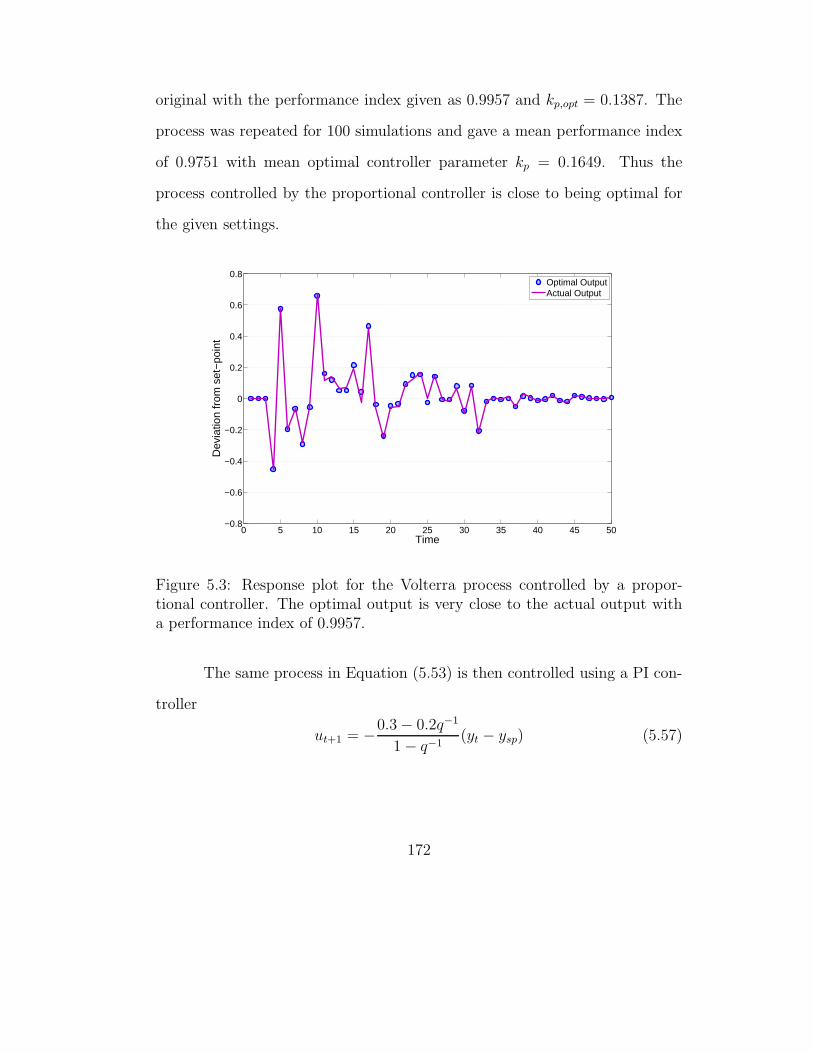
original with the performance index given as 0.9957 and kp,opt = 0.1387. The

process was repeated for 100 simulations and gave a mean performance index

of 0.9751 with mean optimal controller parameter kp = 0.1649. Thus the

process controlled by the proportional controller is close to being optimal for

the given settings.

0 5 10 15 20 25 30 35 40 45 50−0.8

−0.6

−0.4

−0.2

0

0.2

0.4

0.6

0.8

Time

Dev

iatio

n fr

om s

et−

poin

t


Figure 5.3: Response plot for the Volterra process controlled by a propor-tional controller. The optimal output is very close to the actual output witha performance index of 0.9957.

The same process in Equation (5.53) is then controlled using a PI con-

troller

ut+1 = −0.3 − 0.2q−1

1 − q−1(yt − ysp) (5.57)

172

with constraints for k1(= 0.3) and k2(= −0.2) specified as

0.01 ≤ k1 ≤ 3

− 2 ≤ k2 ≤ −0.01(5.58)

The system response for the original and optimized settings are plotted

in Figure (5.4).

0 5 10 15 20 25 30 35 40 45 50−2

−1.5

−1

−0.5

0

0.5

1

1.5

2

Time

Dev

iatio

n fr

om s

et−

poin

t

Actual OutputOptimal Output

Figure 5.4: Response plot for the Volterra process controlled by a PI controller.The optimal output close to the set-point initially but has an offset towardsthe end. The performance index is 0.825.

As seen from the figure, the optimal response is closer to the zero set-

point with the performance index given as 0.825 and [k1, k2] = [0.16,−0.19],

although it shows a small offset. The process was repeated for 100 simulations

and gave a mean performance index of 0.862 with mean optimal controller

173

parameters [k1, k2] = [0.1675,−0.1687]. Thus the process controlled by the

PI controller is suboptimal for the given settings. The results suggest the

controller may be have to be detuned in order to minimize the effect of the

square terms in the process model.

5.6 Results from nonlinear MISO models

We now consider multi-input single-output (MISO) models, which are

linearized so that the effect of the nonlinearity can be ignored or accommo-

dated within the process parameters. The simulation conditions are the same

as before with a white noise sequence is provided to the system at t = 0 and

the system response is plotted for the given settings and the optimized settings

calculated. Each process was found to be nonlinear by the nonlinearity test

based on the Lilliefors exponential distribution test developed earlier.

5.6.1 Lithography dose-focus control

The photolithography process is the most crucial step in semiconductor

manufacturing, where a desired pattern is drawn on the wafer using UV light.

Part of this process is exposure control, where a critical dimension (CD) of

specified length is desired. The CD is dependent mainly on the exposure

dose (expressed in energy per unit area) applied and mildly on the deviation

of the lens focus from the optimal value. The optimal value of the focus is

dependent on the properties of the current substrate layer. A deviation of

zero is ideally desired from the optimum, but usually drifts slowly over a large

174

number of runs. The dependence of CD on the focus and exposure can be

seen in Figure (5.5) (created using ProLith), which shows the CD plotted as

a function of the focus deviation, known as a Bossung curve [17]. Each curve

represents a given exposure dose. It is seen that the process is highly nonlinear

in both the exposure and focus at very high and very low CD values. The CD,

however, shows no dependence on the focus at intermediate CD values. Most

manufacturing tools operate in this region where the process can be considered

as a SISO process with CD depending purely on exposure. But at smaller

CD dimensions the curves have smaller linear sections within which a linear

process model can be used. This demands development of optimal controller

settings for nonlinear process models, since the chip feature size decreases with

advances in manufacturing technology.

The actual CD model is expressed as a function of the inverse depen-

dence on exposure (E) and the focus deviation (F) [120] as

CD =

4∑i=0

3∑j=0

ci,jFi(1 − Es/E)j (5.59)

where Es is a constant representing the minimum exposure dose required for

the process. This constant can be incorporated into the model parameters.

Consider an exposure control process with a target CD of 250 units,

which ignores the focus deviation in the process model

yt = 5700ue,t + et (5.60)

where the output yt is the CD and ue,t is the inverse of exposure dose. The

disturbance et has a white noise input of zero mean and variance 0.1. If uf,t

175

is the focus deviation, the actual model is given by a best-fit regression over

the region of operation as

yt = 6000ue,t − 100uf,t + 1700uf,tue,t − 30u2f,t + et (5.61)

The input ue,t is calculated using Equation (5.60) by inverting the model and

using an EWMA filter with parameter λ = 0.3, assuming a IMA(1,1) distur-

bance model et.

−0.8 −0.6 −0.4 −0.2 0 0.2 0.4 0.650

100

150

200

250

300

350

400

450

500

550

F

CD

1313.51414.51515.51616.51717.51818.51919.52020.521

Window of operation

Figure 5.5: Bossung curves of CD versus focus deviation at different exposurevalues. The dependence of CD is highly nonlinear in both the exposure andfocus, especially at extreme values. The relatively flat regions provide thewindow for process operation.

We use the optimization procedure for this nonlinear process with con-

straints on λ as in Equation (5.51). The focus is varied using a white noise

176

of mean zero and variance 0.01. The results are shown in Figure (5.6). It is

seen that there is an initial jump in the CD which is handled better by the

optimal parameters of λ = 0.87, giving a performance index of 0.625. After

repeating the simulation for 100 white noise sequences for the disturbance, we

get a mean performance index of 0.6193 and λopt = 0.885. Thus, this process

requires higher controller gain for better performance.

0 5 10 15 20 25 30 35 40 45 50240

245

250

255

260

265

270

Time

CD


Figure 5.6: Response plot for the lithography process with only exposure con-trol. The dependence on focus leads to large errors initially, but are correctedquickly by the optimal parameters giving a performance index of 0.625 for theprocess.

177

5.6.2 Back-end-of-line (BEOL) etch

Consider a BEOL etch process which is has two inputs, a tool parameter

ub,t and an etch rate ur,t given by a process model

yt = b0ub,tur,t + et (5.62)

where the output is the etch depth. For a small number of runs, the tool

parameter can be considered as a constant, giving

yt = bur,t + et (5.63)

where b = b0ub,t is considered a constant gain. The input ur,t is calculated

using Equation (5.60) by inverting the model and using an EWMA filter with

parameter λ = 0.3, assuming a IMA(1,1) disturbance model et. The distur-

bance is assumed to have a white noise of zero mean and unit variance as the

input.

We use the optimization procedure for this nonlinear process with con-

straints on λ as in Equation (5.51). The tool parameter is varied using a white

noise of mean zero and variance 0.5. The optimization was found to give op-

timal parameters with biased outputs as in the previous example. Therefore,

the objective function was set to minimize the mean squared error for the

output. The results in Figure (5.7) show a performance index of 0.9511 with

an optimal λ of 0.1545. Repeating the simulation 100 times gives a mean per-

formance index of 0.9113 and λ = 0.1477 as the optimal EWMA parameter.

Thus, the process is slightly sub-optimal for the given settings.

178

It is also observed for both these processes that the magnitude of the

white noise variance plays an important role in determining the optimal pa-

rameters for the EWMA filter.

0 5 10 15 20 25 30 35 40 45 50−3

−2

−1

0

1

2

3

Time

Dev

iatio

n fr

om s

et−

poin

t


Figure 5.7: Response plot for the BEOL etch process with only etch rate undercontrol. The performance index of 0.9511 implies nearly optimal performancefor the process. Note that the MSE was minimized for this example.


In this chapter, we derived a performance metric and optimal param-

eters for PID controllers, when they are used to control nonlinear processes.

Techniques to identify nonlinearity from process data using higher order sta-

tistical methods were first reviewed. A modification was suggested for the non-

linearity test using the Lilliefors test for exponential distributions. This was

179

followed by a review of polynomial NARX model to represent the nonlinearity

in the process and popular techniques for their identification. Methods to find

the best input/output lags and BIBO stability bounds were also reviewed. A

performance monitoring metric was then proposed based on finding optimal

PID parameters that minimize the output variance for a given sequence of

disturbance inputs. This was applied to two SISO processes: an EWMA con-

trolled process from Chapter 2 and a P/PI process from Harris and Yu [68].

The former was found to be optimal for the given settings even though the

linear performance indices in Chapter 2 suggested otherwise. In the latter

example, the process was optimal for the proportional controller settings but

slightly sub-optimal for the PI controller settings. The parameter optimization

was also applied to MISO processes in semiconductor manufacturing where a

nonlinear process is linearized based on operating region. The results showed

that the exposure control process from lithography was sub-optimal while the

BEOL etch process was almost optimal for the given EWMA parameter. In

the future, the methods could be extended to MIMO processes that are non-

linear, such as the chemical mechanical planarization process in semiconductor

manufacturing. In case of very low performance indices for a PID-controlled

nonlinear process, one may consider more complex techniques for process con-

trol such as neural networks. Also, during identification of NARX methods

using OLS techniques, restricted complexity models for control-relevant system

identification [111] could be used.

180

Chapter 6

Conclusions and Future Work

6.1 Key Results

6.1.1 Performance Assessment of Run-to-Run EWMAControllers

In Chapter 2, performance metric was proposed for use in assessing

and monitoring single-loop EWMA control performance using the equivalence

of run-to-run EWMA controllers used in the semiconductor industry with dis-

crete integral controllers used in chemical processing industry (see Prabhu and

Edgar [149]). For this purpose, an iterative solution was derived that gives the

best achievable performance in terms of the closed-loop input-output data and

the process model. An explicit solution was derived as a function of EWMA

parameter λ and the process gain b. A performance index was defined based

on the best achievable performance for use as a realistic performance measure

in the single-loop EWMA control system. It was observed from simulations

that a higher moving window size led to smaller variations in the performance

index value, leading to an optimal window size selection. Gain mismatch was

found to have a larger impact on the performance of the process as compared

to a mismatch in the EWMA filter parameter. Process and metrology delays

were found to have a significant impact on the performance of the EWMA con-

181

troller and therefore need to be accounted for or corrected in order to minimize

their impact on the performance. Bias effects are also prominent as seen from

the simulations with drifting bias and step changes in bias. Nonlinearity on

the process was found to yield different performance metrics depending of the

proximity of the process to the quasi-linear region. As a result the performance

indices were found to vary over a wide range for the same process parameters.

Two etch process and one exposure process from the fab were than studied for

their performance. While each of the three methods was found to be running

close to optimal, the etch process B was seen to be better than the exposure

process and the etch process A. Typical examples of online performance index

charts were provided showing changes in performance over time.

6.1.2 Missing Data Estimation for Run-to-RunEWMA-controlled Processes

In Chapter 3, several methods were developed and compared for es-

timation of missing observations in a time-series from a run-to-run EWMA

controlled process. The minimum norm solution combined with Tikhonov

regularization was compared with simpler alternatives such as the mean of

adjacent observations, using the target value and the last EWMA estimate.

Simulations show that the minimum norm solution performs best in case of

varying sampling rates and gain mismatch. It was better for positive values

of the disturbance model parameter mismatch. A state-space formulation was

developed to reconstruct data affected by missing values using the Kalman

filter. The filter was run in a forward and smoothed fashion to estimate the

182

data. A combination of minimum norm and Kalman filter was proposed as an

improvement over the smoothed Kalman filter, and further simulations were

carried out. The simulations showed the forward Kalman filter with minimum

norm estimates performed better for negative values of the disturbance pa-

rameter mismatch but the minimum norm solution outperformed the Kalman

filter methods for positive values. In case on gain mismatch, the backward

Kalman filter methods were superior only for large mismatch in the gain which

is unlikely in a manufacturing scenario. In case of manufacturing data it was

seen that the minimum norm solution was dominant at low sampling rates,

with other methods better only at very high sampling rates. The method

was successfully applied to manufacturing data with variable delay which is

to be analyzed for performance monitoring purposes. The data reconstruction

based on the minimum norm solution was found to be useful in the case of

some threads, which show an improvement in the performance index trend

over time.

6.1.3 New State Estimation Methods for High-mix SemiconductorManufacturing Processes

In Chapter 4, a new method for state estimation in high-mix manu-

facturing was proposed based on a random walk model for the context states.

Moreover, a moving window approach allows us to use a large amount of histor-

ical data to produce better estimates for the context states. The results show

that with enough data available, this method produces the lowest estimation

error for simulated processes as compared to control threads and JADE. We

183

also combined this random walk approach with the recursive equations of the

Kalman filter to produce estimates, which was found to be useful at lower win-

dow sizes. In case of the individual contexts, it is found that with increasing

number of items per context, the random walk model is the most robust as it

produces the smallest decline in the estimation performance index. The great-

est reduction in performance is seen for the threading method and it is not

recommended for high mix systems. Thus, depending on the process, one can

use either the random walk model, or the random walk estimate-based Kalman

filter method, or JADE. We also applied the method to an industrial exposure

process by extending the random walk model into an integrated moving aver-

age model, preserving the nature of the estimation at the expense of a small

but measurable error. In addition, we used weights to give preference to the

context that was more frequent and therefore more responsible for variations.

As a result, we found that the IMA(1,1) model gave the best estimate for the

given data irrespective of the process window considered.

6.1.4 Identification and Monitoring of PID controlled NonlinearProcesses

In Chapter 5, we derived a performance metric and optimal parameters

for PID controllers, when they are used to control nonlinear processes. Tech-

niques to identify nonlinearity from process data using higher order statistical

methods were first reviewed. A modification was suggested for the nonlinearity

test using the Lilliefors test for exponential distributions. This was followed

by a review of polynomial NARX model to represent the nonlinearity in the

184

process and popular techniques for their identification. Methods to find the

best input/output lags and BIBO stability bounds were also reviewed. A per-

formance monitoring metric was then proposed based on finding optimal PID

parameters that minimize the output variance for a given sequence of distur-

bance inputs. This was applied to two SISO processes: an EWMA controlled

process from Chapter 2 and a P/PI process from Harris and Yu [68]. The

former was found to be optimal for the given settings even though the linear

performance indices in Chapter 2 suggested otherwise. In the latter example,

the process was optimal for the proportional controller settings but slightly

sub-optimal for the PI controller settings. The parameter optimization was

also applied to MISO processes in semiconductor manufacturing where a non-

linear process is linearized based on operating region. The results showed

that the exposure control process from lithography was sub-optimal while the

BEOL etch process was almost optimal for the given EWMA parameter.

6.2 Application in industry

The objective of this work is to provide a framework for the semicon-

ductor industry to implement performance monitoring techniques. We have

analyzed the most commonly used control system, run-to-run control, and the

most common controller used for this purpose, the single parameter EWMA

filter. Implementation of the performance monitoring techniques developed

in Chapter 2 requires that the process be threaded rather than non-threaded.

During implementation, it is necessary to include a data acquisition and for-

185

matting routine to the methodology. Once the data for a particular thread is

acquired, it needs to be standardized in the input-output model format and

arranged in time order. Usually, the data has both process and metrology

timestamp data. This can be utilized to implement the methods developed

in Chapter 3, if the process shows missing data due to reduced sampling or

metrology delays. Once the data is reconstructed, the performance index and

optimal parameters for the given dataset can be calculated. This is summa-

rized in Figure (6.1).

In addition to being a part of the run-to-run performance monitoring

framework, the methods developed for missing value estimation in Chapter 3

may be used in real-time to produce forecasts for incoming batches in a run-

to-run scenario. Since the methods have been shown to be reliable for most

sampling rates, the measurement of outputs in any process (or metrology) can

be reduced to a large extent. This not only reduces the processing time but

also saves the cost of running the metrology tool. We can also use them to

filter measurements if the metrology tool is noisy.

If the process control system in place in the semiconductor manufac-

turing facility is non-threaded, meaning data is not segregated by context, the

methods developed in Chapter 4 may be tested for the given system. It is

seen that model-based approaches are better for a large number of contexts.

Therefore, the random walk model or its modified version based on the IMA

(1,1) model is recommended for the disturbance estimation. In case a recursive

solution is sought, the Kalman filter-based formulation of these methods may

186

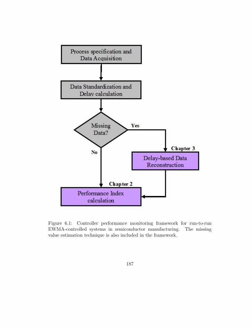
Figure 6.1: Controller performance monitoring framework for run-to-runEWMA-controlled systems in semiconductor manufacturing. The missingvalue estimation technique is also included in the framework.

187

be used at expense to the accuracy of estimation.

In case the process is suspected to be nonlinear and is controlled by

a PID-type controller, the linear process-based performance index becomes

unreliable and therefore we need the techniques developed in Chapter 5 to

analyze such a system. We first need to run tests to confirm the nonlinearity

in the process data using higher order statistical techniques. If the process is

found to be linear, the performance monitoring technique from Chapter 2 is

sufficient. If the process is found to be nonlinear, we classify the nonlinear

process as identifiable using a NARX polynomial model. The identification

can then proceed using orthogonal least squares (OLS) techniques available

in literature with input from the physical model of the system. The modified

performance monitoring technique of Ko and Edgar [100] is now applied with

constraints on the controller parameters to give the nonlinear performance

index. Figure (6.2) provides a summary of such a framework.

6.3 Recommendations for future work

1. The controller performance monitoring techniques for the EWMA con-

troller need to be extended to double-EWMA (or dEWMA) controllers

that are gaining acceptance in the semiconductor industry. This type of

controller is used when the process is known to be subject to large drifts

that cannot be controlled by a single parameter EWMA controller. An

additional parameter which accounts for the drift in the process is used,

but stability regions are now defined in terms of both adjustable param-

188

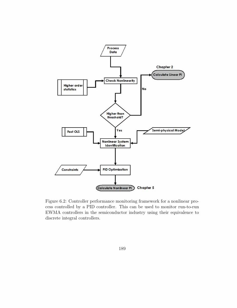
Figure 6.2: Controller performance monitoring framework for a nonlinear pro-cess controlled by a PID controller. This can be used to monitor run-to-runEWMA controllers in the semiconductor industry using their equivalence todiscrete integral controllers.

189

eters, increasing the complexity. Methods also need to be developed for

processes which may exhibit higher order ARIMA disturbance models.

2. Missing data estimation methods incorporating a Bayesian estimation

algorithm can improve the disturbance estimates, because an IMA (1,1)

disturbance sequence can be assumed to behave like a Markov chain

under some conditions. Bayesian inference methods can be used for

state estimation [168] using the Gibbs Sampler [25]. This can possibly

be extended to missing data estimation in combination with adaptive

Monte Carlo integration techniques [24]. These methods are computa-

tionally intensive and can have slow convergence. But they can be used

when analytical solutions using least squares estimation are not possible

for generalized ARIMA (p,d,q) disturbance models that may be present

for some processes. The smoothed Kalman filter solution may also be

applied to wireless communications networks where loss of data occurs

frequently [113, 164].

3. Non-threaded control methods could be compared to a method based on

Bayesian statistics [186], where the Kalman filter covariance matrix is

reset whenever a step disturbance occurs. In case of these methods, we

have neglected the possibility of interactions between context items such

as the tool and the layer. Inclusion of these interaction terms may lead

to nonlinear process models for these disturbances. Therefore, methods

need to be developed for estimation of these complex disturbances. A

190

neural network or decision tree-based approach may be needed in such a

case. Also, a rigorous approach needs to be developed to determine when

production should be switched from threaded to non-threaded control

and vice-versa, according to the product mix.

4. The methods for nonlinear PID controller performance monitoring should

be extended to MIMO processes that are nonlinear, such as the chem-

ical mechanical planarization process in semiconductor manufacturing.

In case of very low performance indices for a PID-controlled nonlinear

process, one may consider more complex techniques for process control

such as neural networks. Also, during identification of NARX methods

using OLS techniques, restricted complexity models for control-relevant

system identification [111] could be used. This greatly eases the opti-

mization of controller parameters.

191

Appendices

192

Appendix A

EWMA and integral feedback control

Consider a pure gain process controlled by a discrete integral feedback

controller with the set-point (ysp) normalized to zero. The controller relates

the current output of the process to the calculated input as

uk+1 = −K(q−1)yk = − kI

1 − q−1yk (A.1)

In case of EWMA forecast-based control [18], we use the input to pro-

vide an adjustment to the actual disturbance ek so that the deviation from

target would be the error εk in the forecast ek instead of the disturbance itself.

Then

yk+1 = buk + ek+1 (A.2)

where b is the gain of the process when an input is applied.

The EWMA forecast is used to predict the next disturbance value based

on the current prediction error as

ek+1 = ek + λ(ek − ek) = ek + λεk (A.3)

with 0 ≤ λ ≤ 1.

193

The input is calculated using this forecast and the apparent gain of the

process

uk = − ek+1

b(A.4)

To prove the equivalence of the two systems as stated in Chapter 2,

consider the difference between successive values of the input and its relation

to the prediction error

uk+1 − uk = − ek+2 − ek+1

b(A.5)

Using Equation (A.3) we get

(1 − q−1)uk+1 = −λbεk (A.6)

Now if the apparent gain b is close to the equivalent gain of the process,

Equation (A.4) substituted in Equation (A.2) leads to

yk = ek − ek = εk (A.7)

Then Equation (A.6) becomes

uk+1 = − λ/b

1 − q−1yk (A.8)

Comparing Equations (A.1) and (A.8), we infer that the EWMA forecast-

based control is equivalent to integral feedback control if the following relation

holds

kI =λ

b(A.9)

subject to accurate determination of the process gain. Note that λ is an

adjustable parameter, so in effect we can tune the integral controller via λ.

194

Appendix B

EWMA control and IMA(1,1) model

The exponentially weighted moving average (EWMA) forecast arises

from a model of expectations adapting to changing conditions. Let et represent

the measured disturbance arising out of the process. Let et represent the

forecast or expectation of et on the basis of information available at time

t− 1. The forecast is changed proportional to the latest observed error in the

disturbance as

ek = ek−1 + λ(ek−1 − ek−1) (B.1)

where 0 ≤ λ ≤ 1. The solution of the above difference equation gives the

formula for the EWMA forecast

ek = λ∞∑i=1

(1 − λ)i−1ek−i (B.2)

Since the weights attached to prior values of et add up to unity, the

forecasting scheme does not in this respect introduce any systematic bias.

Now consider the same disturbance et being written as a linear function of

independent random shocks as follows [132]

ek = ak +∞∑i=1

wiak−i (B.3)

195

the shocks at being i.i.d with mean zero and finite variance. If the distur-

bance follows an integrated moving average (IMA) model of order one, Equa-

tion (B.3) above can be re-written as

ek = ek−1 + ak − θak−1 = ak + (1 − θ)

∞∑i=1

ak−i (B.4)

In order to forecast disturbances based on the IMA model, we need

to find the expectation of ek given ak−1, ak−2, . . .. We also replace ak by its

expected value, which is zero. Thus

ek = (1 − θ)

∞∑i=1

ak−i (B.5)

To relate Equations (B.2) and (B.5) as stated in Chapter 3, we need to

express the forecast in terms of the observed disturbances (ek−1, ek−2, . . .) and

compare the coefficients of the following function

ek =

∞∑j=1

vjek−j (B.6)

Substituting Equation (B.4) we obtain

ek =

∞∑j=1

vj

(ak−j + (1 − θ)

∞∑i=1

ak−i−j

)

= v1ak−1 +

∞∑i=2

(vi + (1 − θ)

i−1∑j=1

vj

)ak−i

(B.7)

Comparing Equations (B.5) and (B.7), we get

v1 = 1 − θ

vi = (1 − θ)(1 −

i−1∑j=1

vj

), i = 2, 3, . . .

(B.8)

196

The first few vi’s then are as follows: v2 = θ(1 − θ), v3 = θ2(1 − θ), . . .

so that

vi = (1 − θ)θi−1, i = 1, 2, . . . (B.9)

Thus we have from Equations (B.6) and (B.9)

ek = (1 − θ)∞∑i=1

θi−1ek−i (B.10)

Comparing Equations (B.2) and (B.10), we get the relationship between

the EWMA forecast and the IMA(1,1) model as

λ = 1 − θ (B.11)

197

Appendix C

Minimum norm solution

In order to derive the solution of the under-determined set of equations

in Chapters 3 and 4, consider a vector-matrix equation

Ax = b (C.1)

where A is an n ×m matrix having rank n, x is an m-vector, and b is an n-

vector. We assume that n < m, i.e., the number of equations is less than the

number of unknown variables, and that Equation (C.1) has an infinite number

of solutions. Then, the solution that minimizes the norm ‖x‖ is given by

xo = ARMb (C.2)

where ARM = AT (AAT )−1. The inverse exists since A is of rank n.

This can be proved as follows [136]. First, note that the norm ‖x‖ can

be written as follows:

‖x‖ = ‖x− xo + xo‖ = ‖xo‖ + ‖x− xo‖ + 2(xo)T (x− xo) (C.3)

198

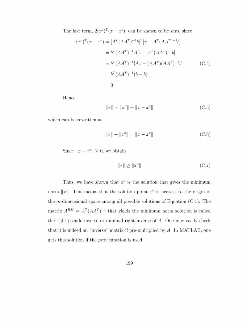
The last term, 2(xo)T (x− xo), can be shown to be zero, since

(xo)T (x− xo) = [AT (AAT )−1b]T [x− AT (AAT )−1b]

= bT (AAT )−1A[x−AT (AAT )−1b]

= bT (AAT )−1[Ax− (AAT )(AAT )−1b]

= bT (AAT )−1(b− b)

= 0

(C.4)

Hence

‖x‖ = ‖xo‖ + ‖x− xo‖ (C.5)

which can be rewritten as

‖x‖ − ‖xo‖ = ‖x− xo‖ (C.6)

Since ‖x− xo‖ ≥ 0, we obtain

‖x‖ ≥ ‖xo‖ (C.7)

Thus, we have shown that xo is the solution that gives the minimum

norm ‖x‖. This means that the solution point xo is nearest to the origin of

the m-dimensional space among all possible solutions of Equation (C.1). The

matrix ARM = AT (AAT )−1 that yields the minimum norm solution is called

the right pseudo-inverse or minimal right inverse of A. One may easily check

that it is indeed an “inverse” matrix if pre-multiplied by A. In MATLAB, one

gets this solution if the pinv function is used.

199

Appendix D

Tikhonov regularization

Consider a vector-matrix equation

Ax = b (D.1)

where A is an n ×m matrix having rank n, x is an m-vector, and b is an n-

vector. We assume that n < m, i.e., the number of equations is less than the

number of unknown variables, and that Equation (D.1) has an infinite number

of solutions. Then, the solution that minimizes the norm ‖x‖ is given by

xo = ARMb (D.2)

where ARM = AT (AAT )−1. The inverse exists since A is of rank n.

The idea of Tikhonov regularization [8] used in Chapter 3 is solving the

following optimization problem

min fγ2(x) (D.3)

where the function

fγ2(x) = ‖Ax− b‖2 + γ2‖x‖2 (D.4)

depends on a positive real parameter γ2. To calculate the minimizer xγ2 of

fγ2 , we reformulate Equation (D.4) as[AγI

]xγ2 =

[b0

](D.5)

200

so that xγ2 minimizes Equation (D.4) only if it is the least squares solution of

Equation (D.5). Multiplying by the transpose we get

[AT γI

] [AγI

]xγ2 =

[AT γI

] [b0

]= AT b (D.6)

The least squares solution is then given by

xγ2 = (ATA + γ2I)−1AT b = Rγb (D.7)

Now consider the singular value decomposition of A = USV T , where U

and V are unitary. S is a diagonal matrix of singular values of A in decreasing

order. The inverse of A is then defined as

A−1 = V S−1UT = V diag(s−1i )UT (D.8)

where s−1i = 0 if si = 0 and i = 1, 2, . . . , n. Then

Rγ = (ATA+ γ2I)−1AT

= (V STUTUSV T + γ2V V T )−1V STUT

=[V (STS + γ2I)V T

]−1V STUT

= V (STS + γ2I)−1STUT

= V diag( si

s2i + γ2

)UT

(D.9)

Thus, as γ → 0 the function fγ2 → A−1b. In addition, we observe that

the norm ‖xγ2‖ is a monotone decreasing function of γ2. It may seem that

the limit γ → 0 is desirable. However, the minimization with positive γ2 is

preferable in case of the constrained least squares problem

minimize ‖Ax− b‖ subject to var(x) = σ2 (D.10)

201

The value of γ can now be adjusted to solve this constrained problem.

The monotone decreasing property of Rγ is used to provide the search direction

in this case.

202

Appendix E

Proof of full rank context matrix

For the random walk model with moving windows in Chapter 4, the

context matrix is of size N ×mN , where N is the moving window size and m

is the number of contexts. Irrespective of the number of items in each context,

the random walk model can be used to extend the columns of each context

according to the moving window size. Thus the context matrix A is given by

A =[A1 A2 . . . Am

](E.1)

where each Ai corresponds to the ith context and is of size N ×N . Since the

maximum rank of a matrix is defined by the minimum of the number of rows

and columns, a full rank A matrix has rank N . Thus in order to prove that A

is always full rank, it is sufficient to prove that each of the sub-matrices Ai is

full rank.

Now consider any such sub-matrix Ai with pi items (∑m

i pi = p, the

number of contexts). Since each row of the matrix is unique as a result of

the random walk model, the contexts are not confounded with each other

as in JADE. Also each item is represented by nj rows in the matrix, where∑pi

j nj = N . Each row contains only zeros and ones, with the number of ones

203

given by the run number of the corresponding context item. For example,

consider the matrix A in Equation (4.23). This context matrix can be divided

into two sub-matrices A1 and A2 by context. Then A1 is given by

A1 =

⎡⎢⎢⎢⎢⎢⎢⎣

1 0 0 0 0 01 1 0 0 0 00 0 0 1 0 00 0 0 1 1 01 1 1 0 0 00 0 0 1 1 1

⎤⎥⎥⎥⎥⎥⎥⎦

(E.2)

The above matrix can be transformed by elementary row operations in-

volving interchange of rows to obtain a block diagonal matrix. Notice that the

matrix can be further subdivided into matrices corresponding to each context

item. In general, any such matrix can be transformed by row interchanges

so that all rows corresponding to a context item are adjacent to each other.

For example, in Equation (E.2), we may use the operations Row3 ↔ Row5

followed by Row4 ↔ Row5 to get

Ar11 =

⎡⎢⎢⎢⎢⎢⎢⎣

1 0 0 0 0 01 1 0 0 0 01 1 1 0 0 00 0 0 1 0 00 0 0 1 1 00 0 0 1 1 1

⎤⎥⎥⎥⎥⎥⎥⎦

(E.3)

where r1 is the number of row interchanges. This matrix is now a block

diagonal matrix with two blocks of size 3×3. Thus, in general we may need ri

row interchanges producing a block diagonal matrix with pi blocks, each block

204

being a square matrix of corresponding size nj . The sub-matrix Ai may now

be represented as

Arii = B1 ⊕B2 ⊕ . . .⊕ Bpi

(E.4)

where ri indicates the number of row interchanges. Now each matrix Bk is a

block lower triangular square matrix of ones. Hence the determinant of each

Bk matrix is 1. Being a block diagonal matrix, the determinant of sub-matrix

Ai is therefore defined by

detAi = (−1)ri

pi∏k

detBk (E.5)

since each row interchanges implies multiplying the determinant of the matrix

by -1. Thus

detAi = (−1)ri (E.6)

Each sub-matrix Ai can be similarly shown to have determinant 1 or -1, and

therefore full rank. Thus the complete context matrix A is also full rank. Then

AAT is always invertible and can be used in Equation (4.25).

205

Bibliography

[1] B. Abraham. Missing observations in time series. Communications in

Statistics - Theory and Methods, 10(16):1643–1653, 1981.

[2] S. Adivikolanu and E. Zafiriou. Extensions and performance/robustness

tradeoffs of the ewma run-to-run controller by using the internal model

control structure. IEEE Transactions on Electronics Packaging Manu-

facturing, 23(1):56–68, 2000.

[3] L. A. Aguirre, M. V. Correa, and C. C. S. Cassini. Nonlinearities in narx

polynomial models: representation and estimation. IEE Proceedings -

Control Theory Applications, 149(4):343–348, 2002.

[4] B. D. A. Anderson and J. B. Moore. Optimal Filtering. Prentice-Hall,

Engelwood Cliffs, N. J., 1st edition, 1979.

[5] C. F. Ansley and R. Kohn. Exact likelihood of vector autoregressive-

moving average process with missing or aggregated data. Biometrika,

70(1):275–278, 1983.

[6] T. A. Badgwell, T. Breedijk, S. G. Bushman, S. W. Butler, S. Chat-

terjee, T. F. Edgar, A. J. Toprac, and I. Trachtenberg. Modeling and

control of microelectronics materials processing. Computers and Chem-

ical Engineering, 19(1):1–41, 1995.

206

[7] W. T. Baumann and W. J. Rugh. Feedback control of nonlinear systems

by extended linearization. IEEE Transactions on Automatic Control,

31(1):40–46, 1986.

[8] A. Ben-Israel and T. N. E. Greville. Generalized Inverses: Theory and

Applications. Springer-Verlag, New York, 2nd edition, 2003.

[9] S. Beveridge. Least squares estimation of missing values in time series.

Communications in Statistics - Theory and Methods, 21(12):3479–3496,

1992.

[10] S. Bezergianni and C. Georgakis. Controller performance assessment

based on minimum and open-loop output variance. Control Engineering

Practice, 8:791–797, 2000.

[11] S. Bezergianni and C. Georgakis. Evaluation of controller performance

use of models derived by subspace identification. International Journal

of Adaptive Control and Signal Processing, 17:527–552, 2003.

[12] C. A. Bode. Run-to-run Control of Overlay and Linewidth in Semicon-

ductor Manufacturing. Phd thesis, The University of Texas at Austin,

2001.

[13] C. A. Bode, B.-S. Ko, and T. F. Edgar. Run-to-run control and perfor-

mance monitoring of overlay in semiconductor manufacturing. Control

Engineering Practice, 12(7):893–900, 2004.

207

[14] C. A. Bode, J. Wang, Q. P. He, and T. F. Edgar. Run-to-run control

and state estimation in high-mix semiconductor manufacturing. Annual

Reviews in Control, 31(2):241–253, 2007.

[15] J. D. Bomberger and D. E. Seborg. Determination of model order

for narx models directly from input-output data. Journal of Process

Control, 8(5):459–468, 1998.

[16] D. S. Boning, W. P. Moyne, T. H. Smith, J. Moyne, R. Telfeyan, A. Hur-

witz, S. Shellman, and J. Taylor. Run by run control of chemical me-

chanical polishing. IEEE Transactions on Semiconductor Manufactur-

ing, 19(4):307–314, 1996.

[17] J. W. Bossung. Projection printing characterization. Proceedings of the

SPIE, 100:80–84, 1977.

[18] G. E. P. Box. Process adjustment and quality control. Total Quality

Management, 4(2):215–228, 1993.

[19] G. E. P. Box and G. M. Jenkins. Time Series Analysis, Forecasting and

Control. Holden-Day, San Francisco, 3rd edition, 1994.

[20] M. W. Braun, S. T. Jenkins, and N. S. Patel. A comparison of supervi-

sory control algorithms for tool/process disturbance tracking. Proceed-

ings of the American Control Conference, pages 2626–2631, 2003.

[21] S. W. Butler. Process control in semiconductor manufacturing. Journal

of Vacuum Science and Technology B, 13(4):1917–1923, 1995.

208

[22] S. W. Butler and J. A. Stefani. Supervisory run-to-run control of a

polysilicon gate etch using in situ ellipsometry. IEEE Transactions on

Semiconductor Manufacturing, 7(2):193–201, 1994.

[23] J. W. Campbell, S. K. Firth, A. J. Toprac, and T. F. Edgar. A com-

parison of run-to-run control algorithms. Proceedings of the American

Control Conference, 3:2150–2155, 2002.

[24] B. P. Carlin, N. G. Polson, and D. S. Stoffer. A monte carlo approach to

nonnormal and nonlinear state-space modeling. Journal of the American

Statistical Association, 87(418):493–500, 1992.

[25] G. Casella and E. I. George. Explaining the gibbs sampler. The Amer-

ican Statistician, 46(3):167–174, 1992.

[26] C. E. Chemali, J. Freudenberg, M. Hankinson, and J. J. Bendik. Run-

to-run critical dimension and sidewall angle lithography control using

the prolith simulator. IEEE Transactions on Semiconductor Manufac-

turing, 17(3):388–401, 2004.

[27] A. Chen and R.-S. Guo. Age-based double ewma controller and its

application to cmp processes. IEEE Transactions on Semiconductor

Manufacturing, 14(1):11–19, 2001.

[28] J. H. Chen, T. W. Kuo, and A. C. Lee. Run-by-run process control of

metal sputter deposition: Combining time series and extended kalman

209

filter. IEEE Transactions on Semiconductor Manufacturing, 20(3):278–

285, 2007.

[29] J. H. Chen and F. Wang. Pls based dewma run-to-run controller for

mimo non-squared semiconductor processes. Journal of Process Control,

17(4):309–319, 2007.

[30] S. Chen, S. A. Billings, and W. Luo. Orthogonal least squares methods

and their application to nonlinear system identification. IEEE Trans-

actions on Automatic Control, 50(5):1873–1896, 1989.

[31] S. Chen and J. Wigger. Fast orthogonal least squares algorithm for effi-

cient subset model selection. IEEE Transactions on Signal Processing,

43(7):1713–1715, 1995.

[32] M. A. A. Choudhury, S. L. Shah, and N. F. Thornhill. Diagnosis of

poor control-loop performance using higher-order statistics. Automat-

ica, 40:1719–1728, 2004.

[33] T. Chowdhury, M. Freeland, O. Krogh, G. Narasimhan, and G. Raghaven-

dra. Propagation of apc models across product boundaries. Proceedings

of the SPIE Conference, 5378:74–80, 2004.

[34] T. Cipra and R. Romera. Kalman filter with outliers and missing ob-

servations. Test, 6(2):379–395, 1997.

210

[35] T. Conway, A. Carlson, and D. Crow. Improving overlay control through

proper use of multi-level query apc. Proceedings of the SPIE Conference,

5044:24–31, 2003.

[36] E. del Castillo. A multivariate self-tuning controller for run-to-run

process control under shift and trend disturbances. IIE Transactions,

28(12):1011–1021, 1996.

[37] E. del Castillo and A. Hurwitz. Run-to-run process control: Literature

review and extensions. Journal of Quality Technology, 29(2):184–196,

1997.

[38] E. del Castillo and R. Rajagopal. A multivariate double ewma process

adjustment scheme for drifting processes. IIE Transactions, 34(12):1055–

1068, 2002.

[39] E. del Castillo and J.-Y. Yeh. An adaptive run-to-run optimizing con-

troller for linear and nonlinear semiconductor processes. IEEE Trans-

actions on Semiconductor Manufacturing, 11(2):285–295, 1998.

[40] A. P. Dempster, N. M. Laird, and D. B. Rubin. Maximum likelihood

from incomplete data via the em algorithm. Journal of the Royal Sta-

tistical Society B, 39(1):1–38, 1977.

[41] L. Desborough and T. J. Harris. Performance assessment measures for

univariate feedback control. Canadian Journal of Chemical Engineering,

70(6):1186–1197, 1992.

211

[42] L. Desborough and T. J. Harris. Performance assessment measures for

univariate feedforward/feedback control. Canadian Journal of Chemical

Engineering, 71(4):605–616, 1993.

[43] H. Diaz and A. Desrochers. Modelling of nonlinear discrete-time systems

for input/output data. Automatica, 24(5):629–641, 1988.

[44] R. Doering and Y. Nishi. Handbook of Semiconductor Manufacturing

Technology. CRC Press, Boca Raton, 2nd edition, 2008.

[45] A. Dzielinski. Bibo stability of narx models. Proceedings of the 7th

Mediterranean Conference on Control and Automation (MED99), pages

1198–1206, 1999.

[46] T. F. Edgar, S. W. Butler, W. J. Campbell, C. Pfeiffer, C. Bode, S. B.

Hwang, K. S. Balakrishnan, and J. Hahn. Automatic control in micro-

electronics manufacturing: Practices, challenges and possibilities. Au-

tomatica, 36(11):1567–1603, 2000.

[47] K. Edwards, J. Zou, and T. Mullins. Handling missing and out-of-order

measurements in run-to-run control applications. Proceedings of the

AEC/APC Symposium XII, 2001.

[48] P.-G. Eriksson and A. J. Isaksson. Some aspects of control loop per-

formance monitoring. Proceedings of the IEEE Conference on Control

Applications, 2:1029–1034, 1994.

212

[49] S.-K. S. Fan. Multiple-input single-output (miso) ridge-optimizing qual-

ity controller for semiconductor manufacturing processes. International

Journal of Production Research, 43(22):4745–4770, 2005.

[50] S.-K. S. Fan, B. C. Jiang, C.-H. Jen, and C.-C. Wang. Siso run-to-

run feedback controller using triple ewma smoothing for semiconductor

manufacturing processes. International Journal of Production Research,

40(13):3093–3120, 2002.

[51] S.-K. S. Fan and C. Y. Wang. On-line tuning system of multivari-

ate dewma control based on a neural network approach. International

Journal of Production Research, 46(13):3459–3484, 2008.

[52] S. K. Firth, W. J. Campbell, A. Toprac, and T. F. Edgar. Just-in-time

adaptive disturbance estimation for run-to-run control of semiconduc-

tor processes. IEEE Transactions on Semiconductor Manufacturing,

19(3):298–315, 2006.

[53] E. J. Godolphin and S. E. Johnson. Decomposition of time series dy-

namic linear models. Journal of Time Series Analysis, 24(5):513–528,

2003.

[54] E. J. Godolphin and K. Triantafyllopoulos. Decomposition of time

series models in state-space form. Computational Statistics and Data

Analysis, 50:2232–2246, 2006.

213

[55] V. Gomez and A. Maravall. Estimation, prediction, and interpolation

for nonstationary series with the kalman filter. Journal of the American

Statistical Association, 89(426):611–624, 1994.

[56] V. Gomez, A. Maravall, and D. Pena. Missing observations in arima

models: Skipping approach versus additive outlier approach. Journal of

Econometrics, 88:341–363, 1999.

[57] R. Good and U. Schulze. Thread state initialization: thread reconstruc-

tion. Proceedings of the AEC/APC Conference, 2006.

[58] R. P. Good. The Stability and Performance of the EWMA and Double-

EWMA Run-to-Run Controllers with Metrology Delay. Phd thesis, The

University of Texas at Austin, 2004.

[59] G. C. Goodwin and A. Feuer. Estimation with missing data. Math-

ematical and Computer Modelling of Dynamical Systems, 5(3):220–244,

1998.

[60] M. J. Grimble. Controller performance benchmarking and tuning using

generalised minimum variance control. Automatica, 38:2111–2119, 2002.

[61] M. J. Grimble. Non-linear generalized minimum variance feedback,

feedforward and tracking control. Automatica, 41:957–969, 2005.

[62] R. Haber and H. Unbehauen. Structure identification of nonlinear dy-

namic systems - a survey on input/output approaches. Automatica,

26(4):651–677, 1990.

214

[63] C. K. Hanish. Run-to-run state estimation in systems with unobservable

states. Proceedings of the AEC/APC Symposium, 2005.

[64] M. Hankinson, T. Vincent, K. B. Irani, and P. P. Khargonekar. Inte-

grated real-time and run-to-run control of etch depth in reactive ion etch-

ing. IEEE Transactions on Semiconductor Manufacturing, 10(1):121–

130, 1997.

[65] T. J. Harris. Assessment of control loop performance. Canadian Jour-

nal of Chemical Engineering, 67(5):856–861, 1989.

[66] T. J. Harris, F. Boudreau, and J. F. MacGregor. Performance assess-

ment of multivariable feedback controllers. Automatica, 32(11):1505–

1518, 1996.

[67] T. J. Harris, C. T. Seppala, and L. D. Desborough. A review of perfor-

mance monitoring and assessment techniques for univariate and multi-

variate control systems. Journal of Process Control, 9(1):1–17, 1999.

[68] T. J. Harris and W. Yu. Controller assessment for a class of non-linear

systems. Journal of Process Control, 17:607–619, 2007.

[69] S. A. Harrison, M. W. Braun, and T. F. Edgar. An evaluation of

the effects of product mix and metrology delay on the performance of

segregated versus threaded ewma control. Proceedings of the AEC/APC

Conference, 2003.

215

[70] A. C. Harvey and R. G. Pierse. Estimating missing observations in

economic time series. Journal of the American Statistical Association,

79:125–131, 1984.

[71] D. F. Heitjan and S. Basu. Distinguishing ’missing at random’ and

’missing completely at random’. The American Statistician, 50(3):207–

213, 1996.

[72] A. Helbig, W. Marquardt, and F. Allgower. Nonlinearity measures:

denition, computation and applications. Journal of Process Control,

10:113–123, 2000.

[73] E. Hernandez and Y. Arkun. Control of nonlinear systems using poly-

nomial arma models. AIChE Journal, 39(3):446–460, 1993.

[74] E. Hernandez and Y. Arkun. Stability of nonlinear polynomial arma

models and their inverse. IBM Journal of Research and Development,

44(5):725–747, 2000.

[75] N. Hernjak and F. J. D. III. Correlation of process nonlinearity with

closed-loop disturbance rejection. Industrial and Engineering Chemistry

Research, 42:4611–4619, 2003.

[76] S. C. Hillmer and G. C. Tiao. An arima-model-based approach to

seasonal adjustment. Journal of the American Statistical Association,

77(377):63–70, 1982.

216

[77] M. J. Hinich. Testing for gaussianity and linearity of a stationary time

series. Journal of Time Series Analysis, 3(3):169–176, 1982.

[78] A. Horch and A. J. Isaksson. A modified index for control performance

assessment. Journal of Process Control, 9:475–483, 1999.

[79] C.-C. Hsu and C.-T. Su. A neural network-based adaptive algorithm

on the single ewma controller. International Journal of Advanced Man-

ufacturing Technology, 23:586–593, 2004.

[80] B. Huang. A pragmatic approach towards assessment of control loop

performance. International Journal of Adaptive Control and Signal Pro-

cessing, 17:589–608, 2003.

[81] B. Huang and S. L. Shah. Performance Assessment of Control Loops:

Theory and Applications. Springer, 1999.

[82] B. Huang, S. L. Shah, and E. K. Kwok. Online control performance

monitoring of mimo processes. Proceedings of the American Control

Conference, 2:1250–1254, 1995.

[83] B. Huang, S. L. Shah, and E. K. Kwok. Good, bad or optimal? perfor-

mance assessment of multivariable processes. Automatica, 33(6):1175–

1183, 1997.

[84] B. Huang, S. L. Shah, and R. Miller. Feedforward plus feedback con-

troller performance assessment of mimo systems. IEEE Transactions

on Control Systems Technology, 8(3):580–587, 2000.

217

[85] H.-P. Huang and J.-C. Jeng. Monitoring and assessment of control per-

formance for single loop systems. Industrial and Engineering Chemistry

Research, 41:1297–1309, 2002.

[86] J. G. Ibrahim, M.-H. Chen, S. R. Lipsitz, and A. H. Herring. Missing-

data methods for generalized linear models: A comparative review. Jour-

nal of the American Statistical Association, 100(469):332–346, 2005.

[87] S. A. Imtiaz. The Treatment of Missing Data in Process Monitoring

and Identification. Phd thesis, University of Alberta, 2007.

[88] A. Ingolfsson and E. Sachs. Stability and sensitivity of an ewma con-

troller. Journal of Quality Technology, 25(4):271–287, 1993.

[89] A. J. Isaksson. Identification of arx-models subject to missing data.

IEEE Transactions on Automatic Control, 38(5):813–819, 1993.

[90] M. Jelali. An overview of control performance assessment technology

and industrial applications. Control Engineering Practice, 14:441–466,

2006.

[91] C.-H. Jen, B. C. Jiang, and S.-K. S.Fan. General run-to-run (r2r)

control framework using self-tuning control for multiple-input multiple-

output (mimo) processes. International Journal of Production Research,

42(20):4249–4270, 2004.

218

[92] X. J. Jing, Z. Q. Lang, and S. A. Billings. New bound characteristics of

narx model in the frequency domain. International Journal of Control,

80(1):140–149, 2007.

[93] T. A. Johansen. On tikhonov reguhrization, bias and variance in non-

linear system identification. Automatica, 33(3):441–446, 1997.

[94] R. H. Jones. Maximum likelihood fitting of arma models to time series

with missing observations. Technometrics, 22:389–395, 1980.

[95] A. Juditsky, H. Hjalmarsson, A. Benveniste, B. Delyon, L. Ljung, J. Sjoberg,

and Q. Zhang. Nonlinear black-box models in system identification:

Mathematical foundations. Automatica, 31(22):1725–1750, 1995.

[96] S. J. Kendra and A. Cinar. Controller performance assessment by fre-

quency domain techniques. Journal of Process Control, 7:181–194, 1997.

[97] B.-S. Ko and T. F. Edgar. Assessment of achievable pi control perfor-

mance for linear processes with dead time. Proceedings of the American

Control Conference, 3:1548–1552, 1998.

[98] B.-S. Ko and T. F. Edgar. Performance assessment of cascade control

loops. AIChE Journal, 46(2):281–291, 2000.

[99] B.-S. Ko and T. F. Edgar. Performance assessment of multivariable

feedback control systems. Proceedings of the American Control Confer-

ence, 6:4373–4377, 2000.

219

[100] B.-S. Ko and T. F. Edgar. Performance assessment of multivariable

feedback control systems. Automatica, 37:899–905, 2001.

[101] B.-S. Ko and T. F. Edgar. Pid control performance assessment: The

single-loop case. AIChE Journal, 50(6):1211–1218, 2004.

[102] R. Kohn and C. F. Ansley. Estimation, prediction, and interpolation

for arima models with missing data. Journal of the American Statistical

Association, 81:751–761, 1986.

[103] S. Lachman-Shalem, B. Grosman, and D. R. Lewin. Nonlinear modeling

and multivariable control of photolithography. IEEE Transactions on


[104] S. P. Lee, R. J. Chou, and S. T. Tseng. Stability and performance of a

double mewma controller for drifted mimo systems. IIE Transactions,

40(7):690–705, 2008.

[105] T. Levin, I. Geier, A. Zhivotovsky, N. Aframiam, and H. Friedlander-

Klar. Automated process control optimization to control low volume

products based on high volume products data. Proceedings of the SPIE

Conference, 5755:145–156, 2005.

[106] K. Li, J.-X. Peng, and E.-W. Bai. A two-stage algorithm for identifica-

tion of nonlinear dynamic systems. Automatica, 42:1189–1197, 2006.

220

[107] K. Li, J.-X. Peng, and G. W. Irwin. A fast nonlinear model identification

method. IEEE Transactions on Automatic Control, 50(8):1211–1216,

2005.

[108] Q. Li, J. R. Whiteley, and R. R. Rhinehart. A relative performance

monitor for process controllers. International Journal of Adaptive Con-

trol and Signal Processing, 17:685–708, 2003.

[109] Q. Li, J. R. Whiteley, and R. R. Rhinehart. An automated performance

monitor for process controllers. Control Engineering Practice, 12:537–

553, 2004.

[110] H. W. Lilliefors. On the kolmogorov-smirnov test for the exponential

distribution with mean unknown. Journal of the American Statistical

Association, 64:387–389, 1969.

[111] W.-M. Ling and D. E. Rivera. A methodology for control-relevant non-

linear system identification using restricted complexity models. Journal

of Process Control, 11:209–222, 2001.

[112] R. J. A. Little. Regression with missing x’s: A review. Journal of the

American Statistical Association, 87(420):1227–1237, 1992.

[113] X. Liu and A. Goldsmith. Kalman filtering with partial observation

losses. Proceedings of the IEEE Conference on Decision and Control,

pages 4180–4186, 2004.

221

[114] G. M. Ljung. A note on the estimation of missing values in time series.

Communications in Statistics - Simulation and Computation, 18(2):459–

465, 1989.

[115] L. Ljung. System Identification: Theory for the User. Prentice-Hall,

Upper Saddle River, N. J., 2nd edition, 1999.

[116] Z. Lu and Y. V. Hui. L1 linear interpolator for missing values in time

series. Annals of the Institute of Statistical Mathematics, 55(1):197–216,

2003.

[117] A. Luceno. Estimation of missing values in possibly partially nonsta-

tionary vector time series. Biometrika, 84(2):495–499, 1997.

[118] C. B. Lynch and G. A. Dumont. Control loop performance monitoring.

Proceedings of the IEEE Conference on Control Applications, pages 835–

840, 1993.

[119] M.-D. Ma and X.-J. Zhu. Control loop performance monitoring. Indus-

trial and Engineering Chemistry Research, 44:3538–3546, 2005.

[120] C. A. Mack and J. D. Byers. Improved model for focus-exposure data

analysis. Proceedings of the SPIE, 5038:396–405, 2003.

[121] V. M. Martinez. Run-by-run control of sti cmp in a high-mix manufac-

turing environment. Proceedings of the AEC/APC Symposium, 2004.

222

[122] V. M. Martinez and T. F. Edgar. Model-based run-to-run controllers for

improved yields. IEEE Control Systems Magazine, pages 46–55, 2006.

[123] P. B. McGiffin and D. N. Murthy. Parameter estimation for auto-

regressive systems with missing observations. International Journal of

Systems Science, 11(9):1021–1034, 1980.

[124] P. B. McGiffin and D. N. Murthy. Parameter estimation for auto-

regressive systems with missing observations - part ii. International

Journal of Systems Science, 12(6):657–663, 1981.

[125] X.-L. Meng and D. B. Rubin. Maximum likelihood estimation via the

ecm algorithm: A general framework. Biometrika, 80(2):267–278, 1993.

[126] X.-L. Meng and D. van Dyk. The em algorithm–an old folk-song sung

to a fast new tune. Journal of the Royal Statistical Society. Series B

(Methodological), 59(3):511–567, 1997.

[127] P. Mhaskar, N. H. El-Farra, and P. D. Christofides. A method for pid

controller tuning using nonlinear control techniques. AIChE Journal,

51(12):3292–3299, 2005.

[128] M. L. Miller. Impact of multi-product and -process manufacturing on

run-to-run control. Proceedings of the SPIE Conference, 3213:138–146,

1997.

223

[129] M. L. Miller, W. J. Campbell, S. K. Firth, and T. F. Edgar. Defining

benchmarks for run-to-run controllers. Proceedings of the AEC/APC

Symposium, 2001.

[130] T. K. Moon. The expectation maximization algorithm. IEEE Signal

Processing Magazine, 13(6):47–60, 1996.

[131] J. Moyne, E. del Castillo, and A. M. Hurwitz. Run-to-Run Control in

Semiconductor Manufacturing. CRC Press, Boca Raton, 2001.

[132] F. Muth. Optimal properties of exponentially weighted forecasts of

time series with permanent and transitory components. Journal of the

American Statistical Association, 55(290):299–306, 1960.

[133] M. Neel, V. M. Martinez, and K. S. Balakrishnan. Run-by-run control

of sti etch in a high-mix manufacturing environment. Proceedings of the

AEC/APC Symposium XVII, 2005.

[134] F. H. Nieto. A note on interpolation of arima processes. Communica-

tions in Statistics - Theory and Methods, 26(10):2381–2392, 1997.

[135] F. H. Nieto and J. Martinez. A recursive approach for estimating miss-

ing observations in an univariate time series. Communications in Statis-

tics - Theory and Methods, 25(9):2101–2116, 1996.

[136] K. Ogata. Modern Control Engineering. Prentice-Hall, Upper Saddle

River, N. J., 3rd edition, 1997.

224

[137] F. Olaleye, B. Huang, and E. Tamayo. Performance assessment of con-

trol loops with time-variant disturbance dynamics. Journal of Process

Control, 14:867–877, 2004.

[138] E. Palmer, W. Ren, C. J. Spanos, and K. Poolla. Control of photore-

sist properties:a kalman filter-based approach. IEEE Transactions on


[139] S.-J. Park, M.-S. Lee, S.-Y. Shin, K.-H. Cho, J.-T. Lim, B.-S. Cho, Y.-H.

Jei, M.-K. Kim, and C.-H. Park. Run-to-run overlay control of steppers

in semiconductor manufacturing systems based on history data analysis

and neural network modeling. IEEE Transactions on Semiconductor

Manufacturing, 18(4):605–613, 2005.

[140] A. J. Pasadyn and T. F. Edgar. Observability and state estimation

for multiple product control in semiconductor manufacturing. IEEE

Transactions on Semiconductor Manufacturing, 18(4):592–604, 2005.

[141] N. Patel and S. T. Jenkins. Adaptive optimization of run-to-run con-

trollers: The ewma example. IEEE Transactions on Semiconductor

Manufacturing, 13(1):97–107, 2000.

[142] N. S. Patel and C. K. Hanish. Effect of out of order measurements in

process control. Proceedings of the AEC/APC Symposium, 2003.

[143] R. S. Patwardhan and S. L. Shah. Issues in performance diagnostics of

model-based controllers. Journal of Process Control, 12:413–427, 2002.

225

[144] D. Pena and G. C. Tiao. A note on likelihood estimation of missing

values in time series. The American Statistician, 45(3):212–213, 1991.

[145] J. Penzer and B. Shea. The exact likelihood of an autoregressive-moving

average model with incomplete data. Biometrika, 84(4):919–928, 1997.

[146] J. Penzer and B. Shea. Finite sample prediction and interpolation for

arima models with missing data. Journal of Forecasting, 18:411–419,

1999.

[147] C. Pfeiffer, C. Stager, C. Dang, B. Freeborn, and J. C. Arnold. Run by

run control of oxide cmp tools in a high-mix environment. Proceedings

of the AEC/APC Symposium, 2001.

[148] L. Piroddi and W. Spinelli. An identification algorithm for polyno-

mial narx models based on simulation error minimization. International

Journal of Control, 76(17):1767–1781, 2003.

[149] A. V. Prabhu and T. F. Edgar. Performance assessment of run-to-run

ewma controllers. IEEE Transactions on Semiconductor Manufactur-

ing, 20(4):381–385, 2007.

[150] T. Proietti. Missing data in time series: A note on the equivalence of the

dummy variable and the skipping approaches. Statistics and Probability

Letters, 78:257–264, 2008.

[151] S. J. Qin. Controller performance monitoring a review and assessment.

Computers and Chemical Engineering, 23(2):173–186, 1998.

226

[152] S. J. Qin, G. Cherry, R. Good, J. Wang, and C. A. Harrison. Semi-

conductor manufacturing process control and monitoring: A fab-wide

framework. Journal of Process Control, 16(3):179–191, 2006.

[153] T. S. Rao and M. M. Gabr. A test for linearity and stationarity of time

series. Journal of Time Series Analysis, 1(1):145–158, 1980.

[154] D. B. Rubin. Inference and missing data. Biometrika, 63:581–592,

1976.

[155] D. B. Rubin. Multiple imputation after 18+ years. Journal of the

American Statistical Association, 91:473–489, 1996.

[156] E. Sachs, R.-S. Guo, S. Ha, and A. Hu. Process control system for

vlsi fabrication. IEEE Transactions on Semiconductor Manufacturing,

4(2):134–144, 1991.

[157] E. Sachs, A. Hu, and A. Ingolfsson. Run by run process control: Com-

bining spc and feedback control. IEEE Transactions on Semiconductor

Manufacturing, 8(1):26–43, 1995.

[158] T. I. Salsbury. A practical method for assessing the performance of con-

trol loops subject to random load changes. Journal of Process Control,

15(4):393–405, 2005.

[159] J. D. Sargan and E. G. Drettakis. Missing data in an autoregressive

model. International Economic Review, 15(1):39–58, 1974.

227

[160] J. L. Schafer and J. W. Graham. Missing data: Our view of the state

of the art. Psychological Methods, 7(2):147–177, 2002.

[161] D. E. Seborg, T. F. Edgar, and D. A. Mellichamp. Process Dynamics

and Control. Wiley, New York, 2nd edition, 2004.

[162] S. T. Seo, K. S. Lee, and D. R. Yang. Run-to-run control of induc-

tively coupled c2f6 plasma etching of sio2: Multivariable controller de-

sign and numerical application. Korean Journal of Chemical Engineer-

ing, 23(2):199–202, 2006.

[163] E. I. Silva and M. E. Salgado. Performance bounds for feedback control

of non-minimum phase mimo systems with arbitrary delay structure.

IEE Proceedings in Control Theory Applications, 152(2):211–219, 2005.

[164] B. Sinopoli, L. Schenato, M. Franceschetti, K. Poolla, M. I. Jordan, and

S. S. Sastry. Kalman filtering with intermittent observations. IEEE

Transactions on Automatic Control, 49(9):1453–1464, 2004.

[165] T. H. Smith and D. S. Boning. Artificial neural network exponentially

weighted moving average controller for semiconductor processes. Jour-

nal of Vacuum Science and Technology A - Vacuum Surfaces and Films,

15(3):1377–1384, 1997.

[166] T. H. Smith and D. S. Boning. A self-tuning ewma controller utiliz-

ing artificial neural network function approximation techniques. IEEE

228

Transactions on Components Packaging Manufacturing Technology, 20(2):121–

132, 1997.

[167] T. H. Smith, D. S. Boning, J. Stefani, and S. W. Butler. Run by run ad-

vanced process control of metal sputter deposition. IEEE Transactions

on Semiconductor Manufacturing, 11(2):276–284, 1998.

[168] J. C. Spall. Estimation via markov chain monte carlo. IEEE Control

Systems Magazine, pages 34–45, 2003.

[169] A. J. Stack and F. J. Doyle. The optimal control structure: an ap-

proach to measuring control-law nonlinearity. Computers and Chemical

Engineering, 21(9):1009–1019, 1997.

[170] N. Stanfelj, T. E. Marlin, and J. F. MacGregor. Monitoring and di-

agnosing process control performance: The single-loop case. Industrial

and Engineering Chemistry Research, 32(2):301–314, 1993.

[171] P. Stoica, L. Xu, and J. Li. A new type of parameter estimation al-

gorithm for missing data problems. Statistics and Probability Letters,

75:219–229, 2005.

[172] A. J. Su, C. C. Yu, and B. A. Ogunnaike. On the interaction between

measurement strategy and control performance in semiconductor man-

ufacturing. Journal of Process Control, 18(3-4):266–276, 2008.

229

[173] A. P. Swanda and D. E. Seborg. Controller performance assessment

based on setpoint response data. Proceedings of the American Control

Conference, pages 3863–3867, 1999.

[174] T. A. Tanzer, R. J. Chong, and M. A. Purdy. Standardized method

for controller performance monitoring. Proceedings of the AEC/APC

Symposium XVI, 2004.

[175] T. Thyagarajan, C.-C. Yu, and H.-P. Huang. Assessment of controller

performance: a relay feedback approach. Chemical Engineering Science,

58:497–512, 2003.

[176] A. Toprac and Y. Wang. Solving the high-mix control problem. Pro-

ceedings of the AEC/APC Symposium, 2004.

[177] S. T. Tseng, W. M. Song, and Y. C. Chang. An initial intercept it-

eratively adjusted (iiia) controller: An enhanced double ewma feedback

control scheme. IEEE Transactions on Semiconductor Manufacturing,

18(3):448–457, 2005.

[178] S. T. Tseng, F. Tsung, and P. Y. Liu. Variable ewma run-to-run con-

troller for drifted processes. IIE Transactions, 39(3):291–301, 2007.

[179] S. T. Tseng, A. B. Yeh, F. Tsung, and Y.-Y. Chan. A study of variable

ewma controller. IEEE Transactions on Semiconductor Manufacturing,

16(4):633–643, 2003.

230

[180] M. L. Tyler and M. Morari. Performance monitoring of control systems

using likelihood ratio methods. Proceedings of the American Control

Conference, pages 1245–1249, 1995.

[181] O. A. Vanli, N. S. Patel, M. Janakiram, and E. del Castillo. Model

context selection for run-to-run control. IEEE Transactions on Semi-

conductor Manufacturing, 20(4):506–516, 2007.

[182] W. F. Velicer and S. M. Colby. A comparison of missing data pro-

cedures for arima time-series analysis. Educational and Psychological

Measurement, 65(4):596–615, 2005.

[183] S. Wan and B. Huang. Robust performance assessment of feedback

control systems. Automatica, pages 33–46, 2002.

[184] X. Wan, A. Zhou, F. Zhang, J. Li, X. Gu, E. Mos, A. Kisteman, V. Wang,

and R. Schuurhuis. Overlay advanced process control for foundry appli-

cation. Proceedings of the SPIE Conference, 5375:735–743, 2004.

[185] G. J. Wang and C. H. Yu. Developing a neural network-based run-to-run

process controller for chemical-mechanical planarization. International

Journal of Advanced Manufacturing Technology, 28(9):899–908, 2006.

[186] J. Wang, Q. P. He, and T. F. Edgar. On state estimation in high-

mix semiconductor manufacturing using a singular gauss-markov model.

Journal of Process Control, to be published, 2008.

231

[187] J. Wang, Q. P. He, S. J. Qin, C. A. Bode, and M. A. Purdy. Recursive

least squares estimation for run-to-run control with metrology delay and

its application to sti etch process. IEEE Transactions on Semiconductor

Manufacturing, 18(2):309–319, 2005.

[188] M. West. Time series decomposition. Biometrika, 84(2):489–494, 1997.

[189] G. N. Wilkinson. Estimation of missing values for the analysis of in-

complete data. Biometrics, 14(2):257–286, 1958.

[190] H. Xia, P. Majecki, A. Ordys, and M. Grimble. Performance assessment

of mimo systems based on i/o delay information. Journal of Process

Control, 16:373–383, 2006.

[191] F. Xu and B. Huang. Performance monitoring of siso control loops sub-

ject to ltv disturbance dynamics: An improved lti benchmark. Journal


[192] J. Yuan. Testing linearity for stationary time series using the sample

interquartile range. Journal of Time Series Analysis, 21(6):713–722,

1999.

[193] H. Yue, J. Stuber, J. Lohse, and D. Hui. Run-to-run exposure controller

and fault detection in a high-mix development and manufacturing envi-

ronment. Proceedings of the AEC/APC Symposium, 2005.

232

[194] Y. Zheng, Q.-H. Lin, D. S.-H. Wang, S.-S. Jang, and K. Hui. Stability

and performance analysis of mixed product run-to-run control. Journal


233

Vita

Amogh Vishwanath Prabhu was born in Mumbai (formerly Bombay),

Maharashtra, India on the 10th of March, 1983. He received his Secondary

School Certificate (SSC) from St. Xavier’s High School in Mumbai, Maharash-

tra in March, 1998 and his Higher Secondary Certificate (HSC) from Sathaye

College in Mumbai, Maharashtra in February, 2000, both from the Maharash-

tra State Board of Secondary and Higher Secondary Education Exams. He

entered the Mumbai University Institute of Chemical Technology (MUICT) in

September, 2000 and received his Bachelor of Chemical Engineering degree in

May, 2004. Mr. Prabhu entered graduate school at the University of Texas at

Austin in August, 2004 and worked as a graduate research assistant. During

his study at the University of Texas at Austin, he also served as a Teaching

Assistant in the fall of 2005 and a graduate level co-op at Advanced Micro

Devices, Inc. during the spring and the summer of 2006, and the spring of

2007.

Permanent address: 4539 Guadalupe StAustin, Texas 78751

This dissertation was typeset with LATEX† by the author.

†LATEX is a document preparation system developed by Leslie Lamport as a specialversion of Donald Knuth’s TEX Program.

234

Date post:	21-Mar-2022
Category:	Documents
Upload:	others
View:	1 times
Download:	0 times

Copyright by Amogh V. Prabhu 2008

Documents