48
Course eval results • More applications • Last question – Luging: 0.5 – Curling: 1.5 – Figure skating: 2 – Ice fishing: 6.5 – Foosball: 0.5
| Date post: | 22-Dec-2015 |
| Category: |
Documents |
| View: | 217 times |
| Download: | 2 times |

Course eval results
• More applications
• Last question– Luging: 0.5– Curling: 1.5– Figure skating: 2– Ice fishing: 6.5– Foosball: 0.5

Nelson-Oppen review
• f(x – 1) – 1 = x + 1 Æ f(y) + 1 = y – 1 Æ y + 1 =x
`² Q
EDI
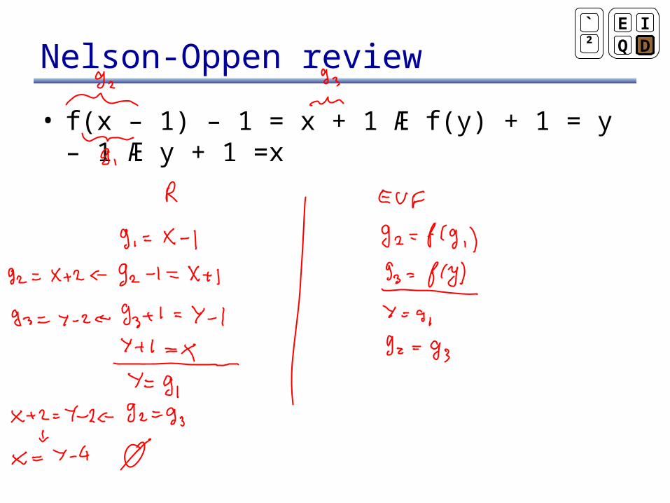
Nelson-Oppen review
• f(x – 1) – 1 = x + 1 Æ f(y) + 1 = y – 1 Æ y + 1 =x
`² Q
EDI

Drawback of Nelson-Oppen`² Q
EDI

Drawback of Nelson-Oppen
• Theory must be convex, otherwise must backtrack
• Some large overheads:– Each decision procedure must maintain its own
equalities– There are a quadratic number of equalities that can
be propagated
`² Q
EDI
Shostak’s approach
• Alternate approach to combining theories that addresses some of the performance drawbacks of Nelson-Oppen
• Published in 1984 in JACM, but the original formulation was later found to be flawed in several ways
• Long line of work to correct these mistakes
• Several papers cite an Unpublished manuscript by Crocker from 1988 showing that Shostak is 10 times faster than Nelson-Oppen
• Recent paper by Barrett, Dill and Stump in 2002 shows that Shostak can be seen as a special case of Nelson-Oppen
`² Q
EDI

Shostak’s approach
• Shostak is used in a variety of theorem provers, including PVS and SVC
• We will cover the intuition behind Shostak’s approach, but we won’t see the details
`² Q
EDI
The key idea in Shostak
• Keep one congruence closure data-structure S for all theories
• Each individual decision procedure finds new equalities based on the ones that are already in S
• As individual decision procedures find equalities, add them to S
`² Q
EDI
Adding equalities to S
• Straightforward to encode equalities over uninterpreted function symbols in S– Since S is a congruence-closure data structure, since
congruence closure was originally intended for exactly these kinds of equalities
• Interpreted functions symbols require more care– For example, an equality y + 1 = x +2 cannot be
processed by simply putting y + 1 and x + 2 in the same equivalence class, since the original equality in fact entails a multitude of equalities, such as y = x + 1, y – 1 = x, y -2 = x -1, etc.
`² Q
EDI

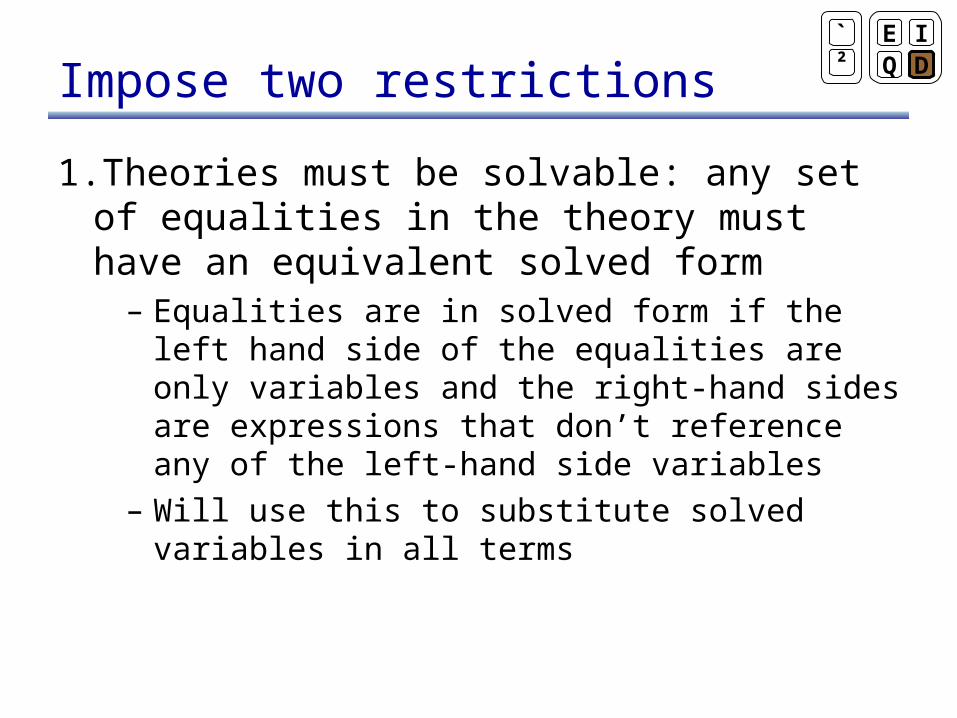
Impose two restrictions
1.Theories must be solvable: any set of equalities in the theory must have an equivalent solved form
– Equalities are in solved form if the left hand side of the equalities are only variables and the right-hand sides are expressions that don’t reference any of the left-hand side variables
x + y = z + 3
x – y = 3z + 1
`² Q
EDI
Impose two restrictions
1.Theories must be solvable: any set of equalities in the theory must have an equivalent solved form
– Equalities are in solved form if the left hand side of the equalities are only variables and the right-hand sides are expressions that don’t reference any of the left-hand side variables
– Will use this to substitute solved variables in all terms
`² Q
EDI

Impose two restrictions
2.Theory must be canonizable– There is a canonizer function such that if a = b, then
(a) is syntactically equal to (b)– Canonizer for linear arithmetic: transform terms into
ordered monomials– (a + 3c + 4b + 3 + 2a + 4) = 3a + 4b + 3c + 7– The intuition is that by canonizing all terms, we can
then use syntactic equality to determine semantic equality
`² Q
EDI
Putting it all together
• f(x – 1) – 1 = x + 1 Æ f(y) + 1 = y – 1 Æ y + 1 =x
`² Q
EDI
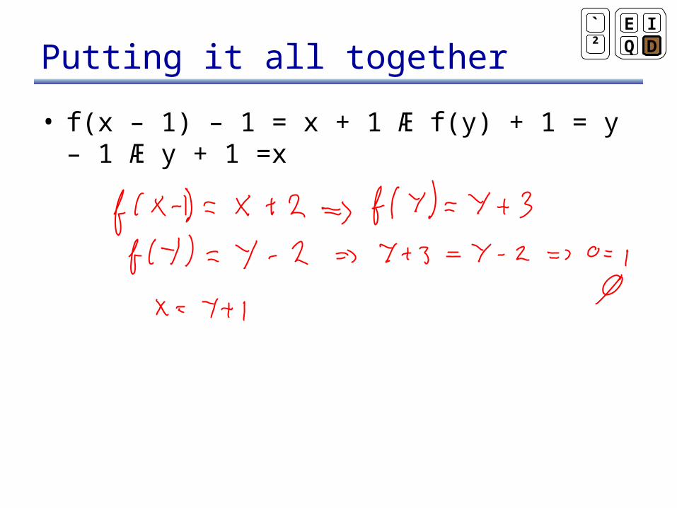
Putting it all together
• f(x – 1) – 1 = x + 1 Æ f(y) + 1 = y – 1 Æ y + 1 =x
`² Q
EDI
ACL2 paper
• ACL2 architecture– Given a goal, ACL2 has a set of strategies it can
apply– For example: rewriting, simplification, induction– Applying a strategy produces sub-goals from the
given goal– Each sub-goal needs to be proven recursively
`² Q
EDI
Adding linear arithmetic
• First attempt was to just use the decision procedures directly as a strategy
• Not found to be useful, because it was rarely the case that the goal would reduce to TRUE using linear arithmetic
• Rather, they found they needed to add linear arithmetic in the rewrite system
• A rewrite rule: A ) T1 = T2
– To trigger, need to establish A– They often needed linear arithmetic to establish A
`² Q
EDI
Keep a linear arith DB
• A rewrite rule: A ) T1 = T2
• To establish A, add : A to the current database of linear equalities and inequalities
• If an inconsistency is reached, we know A holds
• We can perform the rewrite
• Remove : A from the database, and add A
`² Q
EDI
Instantiating axioms
• This was an improvement, but they then found that interpreted function symbols were not handled properly:– L · min(A) Æ 0 < K ) L < max(A) + K
• The problem is that min and max are uninterpreted– We need to know that min(A) · max(A)
• This boils down to finding the right instantiations of the Lemma 8 X . min(X) · max(X)
`² Q
EDI
Instantiating quantifiers
• They use a form of matching
• Key multiplicands in the database of linear arithmetic are used to instantiate Lemmas
• Have heuristics to avoid infinite expansion
`² Q
EDI

So far
Proof-system search ( ` )
Interpretation search ( ² ) Quantifiers
Equality
Decisionprocedures
Induction
Cross-cutting aspectsMain search strategy
E-graph Communication between decision procedures and between prover and decision procedures
•DPLL•Backtracking•Incremental
SAT
Matching
Next
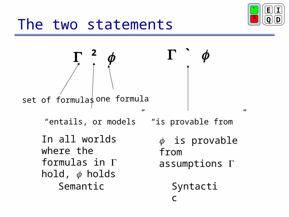
The two statements
` ²
set of formulas one formula
“entails, or models” “is provable from ”
In all worlds where the formulas in hold, holds
is provable from assumptions
Semantic Syntactic
`² Q
EDI
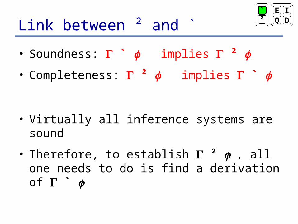
Link between ² and `
• Soundness: ` implies ²
• Completeness: ² implies `
• Virtually all inference systems are sound
• Therefore, to establish ² , all one needs to do is find a derivation of `
`² Q
EDI
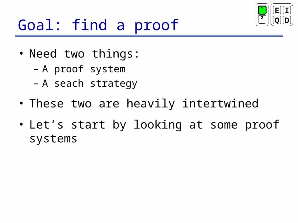
Goal: find a proof
• Need two things:– A proof system– A seach strategy
• These two are heavily intertwined
• Let’s start by looking at some proof systems
`² Q
EDI
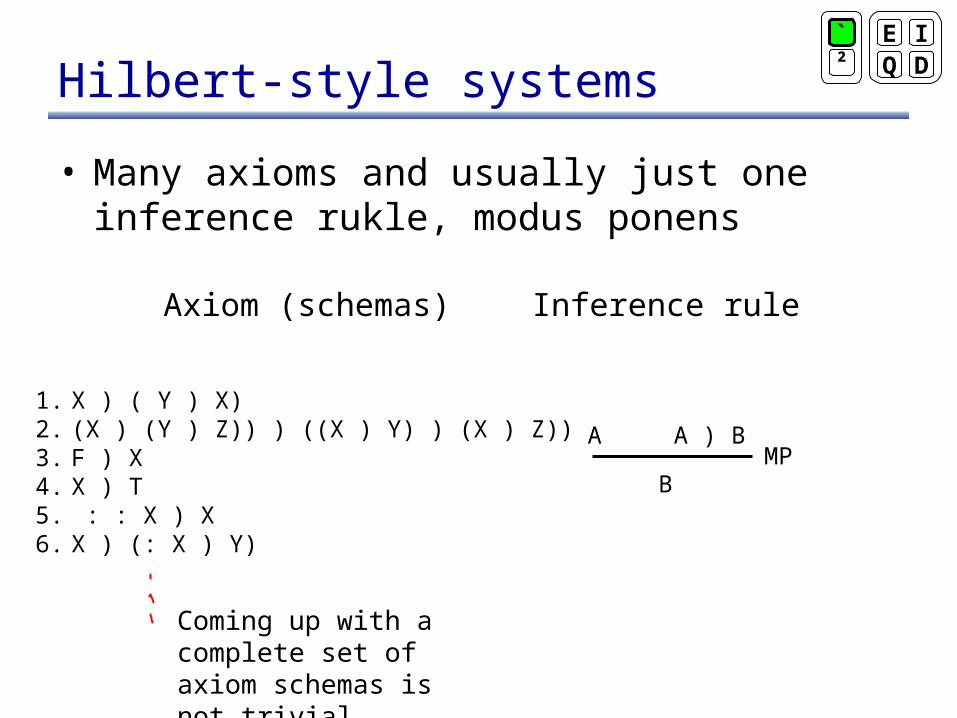
Hilbert-style systems
• Many axioms and usually just one inference rukle, modus ponens
1. X ) ( Y ) X)2. (X ) (Y ) Z)) ) ((X ) Y) ) (X ) Z))3. F ) X4. X ) T5. : : X ) X6. X ) (: X ) Y)
Axiom (schemas)
A A ) B
B MP
Inference rule
Coming up with a complete set of axiom schemas is not trivial
`² Q
EDI
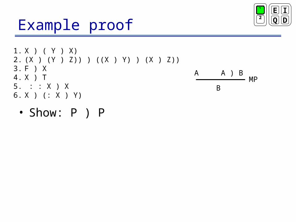
Example proof
• Show: P ) P
1. X ) ( Y ) X)2. (X ) (Y ) Z)) ) ((X ) Y) ) (X ) Z))3. F ) X4. X ) T5. : : X ) X6. X ) (: X ) Y)
A A ) B
B MP
`² Q
EDI
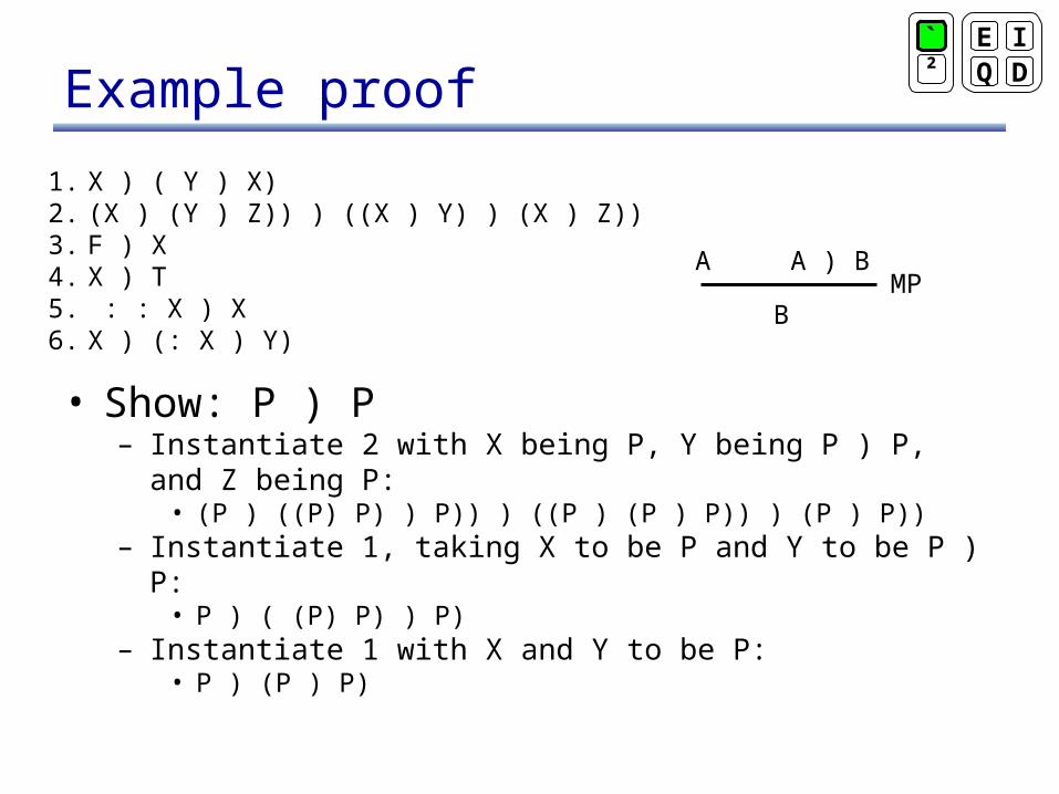
Example proof
• Show: P ) P– Instantiate 2 with X being P, Y being P ) P, and Z being P:
• (P ) ((P) P) ) P)) ) ((P ) (P ) P)) ) (P ) P))– Instantiate 1, taking X to be P and Y to be P ) P:
• P ) ( (P) P) ) P)– Instantiate 1 with X and Y to be P:
• P ) (P ) P)
1. X ) ( Y ) X)2. (X ) (Y ) Z)) ) ((X ) Y) ) (X ) Z))3. F ) X4. X ) T5. : : X ) X6. X ) (: X ) Y)
A A ) B
B MP
`² Q
EDI

Example proof
• Show: P ) P– Instantiate 2 with X being P, Y being P ) P, and Z being P:
• (P ) ((P) P) ) P)) ) ((P ) (P ) P)) ) (P ) P)) *– Instantiate 1, taking X to be P and Y to be P ) P:
• P ) ( (P) P) ) P) **– Instantiate 1 with X and Y to be P:
• P ) (P ) P) ***– Apply MP on * and **:
• (P ) (P ) P)) ) (P ) P) ****– Apply MP on *** and ****:
• P ) P
1. X ) ( Y ) X)2. (X ) (Y ) Z)) ) ((X ) Y) ) (X ) Z))3. F ) X4. X ) T5. : : X ) X6. X ) (: X ) Y)
A A ) B
B MP
`² Q
EDI
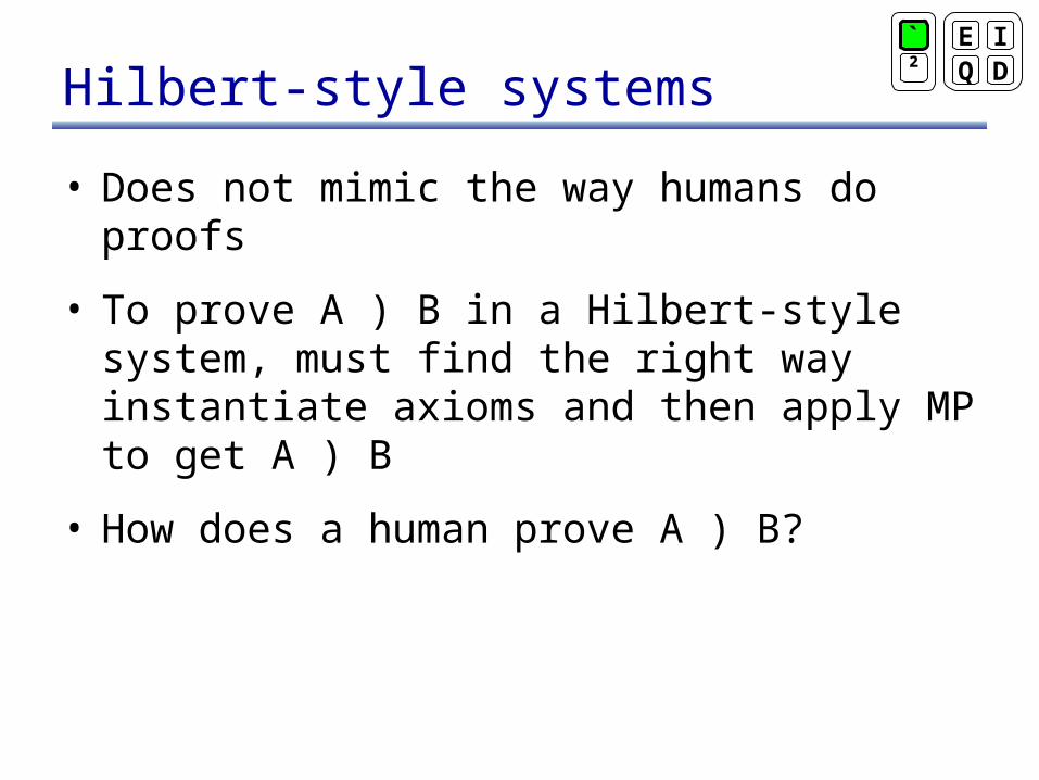
Hilbert-style systems
• Does not mimic the way humans do proofs
• To prove A ) B in a Hilbert-style system, must find the right way instantiate axioms and then apply MP to get A ) B
• How does a human prove A ) B?
`² Q
EDI

Hilbert-style systems
• Does not mimic the way humans do proofs
• To prove A ) B in a Hilbert-style system, must find the right way instantiate axioms and then apply MP to get A ) B
• How does a human prove A ) B?
• Assume A, and show B
• In this context, showing P ) P is very easy
`² Q
EDI
Natural deduction
• The system of natural deduction was developed by Gentzen in 1935 out of dissatisfaction with Hilbert-style axiomatic systems, which did not closely mirror the way humans usually perform proofs
• Gentzen wanted to create a system that mimics the “natural” way in which humans think
`² Q
EDI
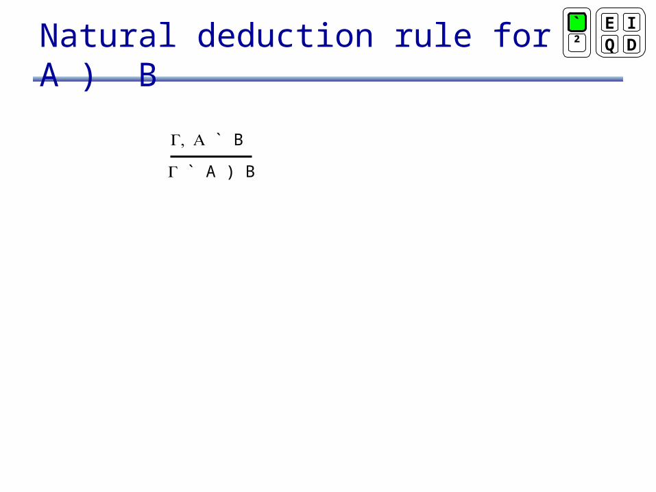
Natural deduction rule for A ) B
` B
` A ) B
`² Q
EDI
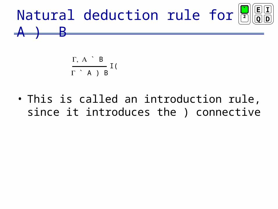
Natural deduction rule for A ) B
• This is called an introduction rule, since it introduces the ) connective
` B
` A ) B (I
`² Q
EDI
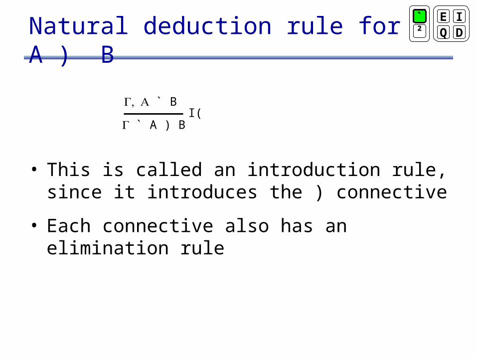
Natural deduction rule for A ) B
• This is called an introduction rule, since it introduces the ) connective
• Each connective also has an elimination rule
` B
` A ) B (I
`² Q
EDI

Natural deduction rule for A ) B
• This is called an introduction rule, since it introduces the ) connective
• Each connective also has an elimination rule
` B
` A ) B (I
` A ` A ) B
` B )E
`² Q
EDI
Natural deduction
` A Æ B
` A Æ BÆI ÆE
` A Ç B ÇI
` A Ç BÇE
`² Q
EDI

Natural deduction
` : A :I
` : A :E
` F FI
` F FE
` T TI
` T TE
`² Q
EDI
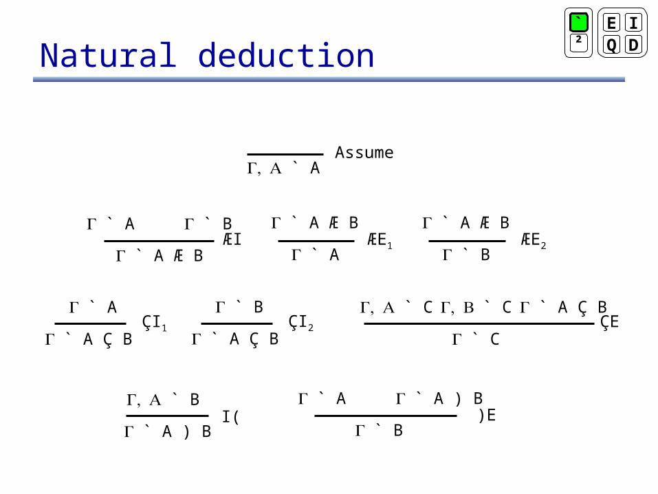
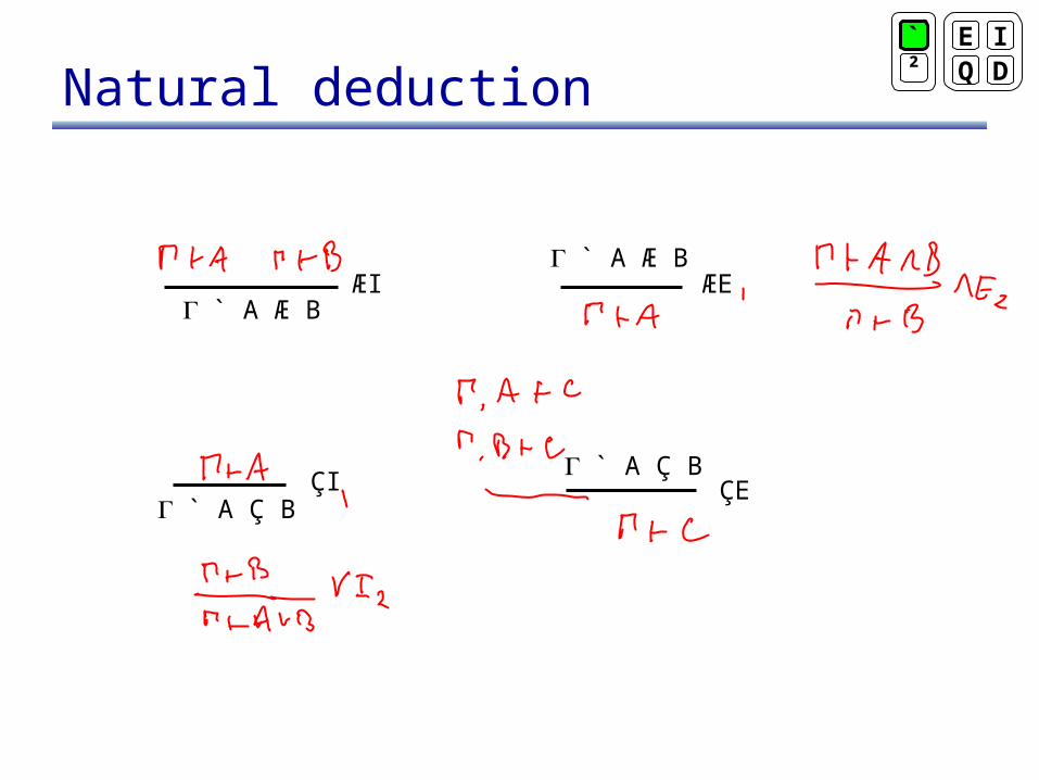
Natural deduction
` A ` B
` A Æ B
` A Æ B
` A
` A Æ B
` B
` B
` A ) B
` A ` A ) B
` B
` A
ÆI ÆE1 ÆE2
Assume
(I )E
` A
` A Ç B ÇI1
` B
` A Ç B ÇI2
` A Ç B
` C ÇE
` C ` C
`² Q
EDI
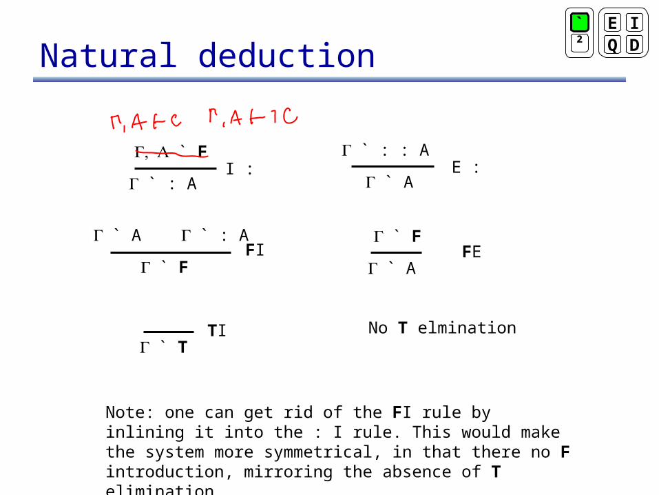
Natural deduction
` F
` : A :I
` : : A
` A :E
` A ` : A
` F FI
` F
` A FE
` T TI No T elmination
Note: one can get rid of the FI rule by inlining it into the : I rule. This would make the system more symmetrical, in that there no F introduction, mirroring the absence of T elimination
`² Q
EDI

Once we have a proof system
• Once we have a proof system, the goal is to devise a search algorithm to find a proof
• Search algorithm sound: proofs that it finds are correct
• Search algorithm complete: if there is a proof, the algorithm will find it
• These soundness and completeness properties relate the search algorithm to the proof system, and should not be confused with soundness and completeness of the proof system
`² Q
EDI

Two main strategies
• Given a formula to prove:– One can start from axioms and apply inference rules
forward, until a derivation of the given formula is found
– One can start from the formula to prove (the goal) and apply inference rules backward to find sub-goals until all sub-goals are axioms
• The forward version is sometimes called forward chaining, the backward version backward chaining
`² Q
EDI
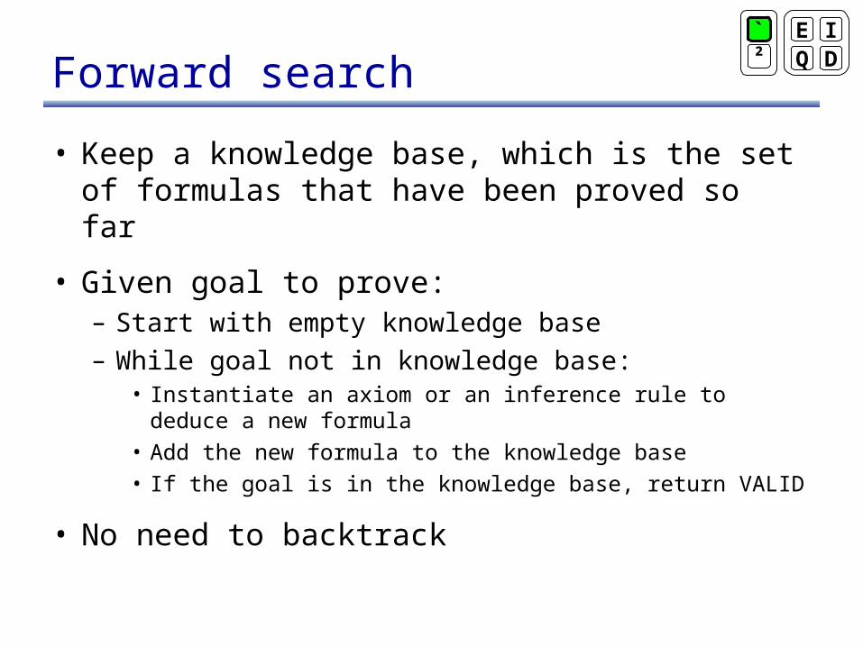
Forward search
• Keep a knowledge base, which is the set of formulas that have been proved so far
• Given goal to prove:– Start with empty knowledge base– While goal not in knowledge base:
• Instantiate an axiom or an inference rule to deduce a new formula
• Add the new formula to the knowledge base• If the goal is in the knowledge base, return VALID
• No need to backtrack
`² Q
EDI
Forward search -- refutation
• Start with knowledge base being the negation of the goal
• While enlarging the knowledge base, if F becomes part of the knowledge, then return VALID
`² Q
EDI
Backward search
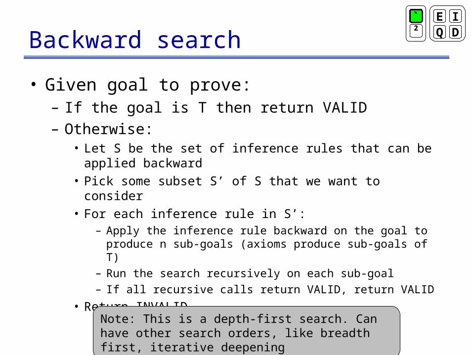
• Given goal to prove:– If the goal is T then return VALID– Otherwise:
• Let S be the set of inference rules that can be applied backward
• Pick some subset S’ of S that we want to consider• For each inference rule in S’:
– Apply the inference rule backward on the goal to produce n sub-goals (axioms produce sub-goals of T)
– Run the search recursively on each sub-goal
– If all recursive calls return VALID, return VALID
• Return INVALID
`² Q
EDI
Note: This is a depth-first search. Can have other search orders, like breadth first, iterative deepening
Proofs
• One can easily adapt these algorithms to keep track of the proof tree, so that a proof can be produced if the goal is valid
• Contrast this with our backtracking search in the semantic domain, where generating a proof was not as simple
`² Q
EDI
Non-determinism
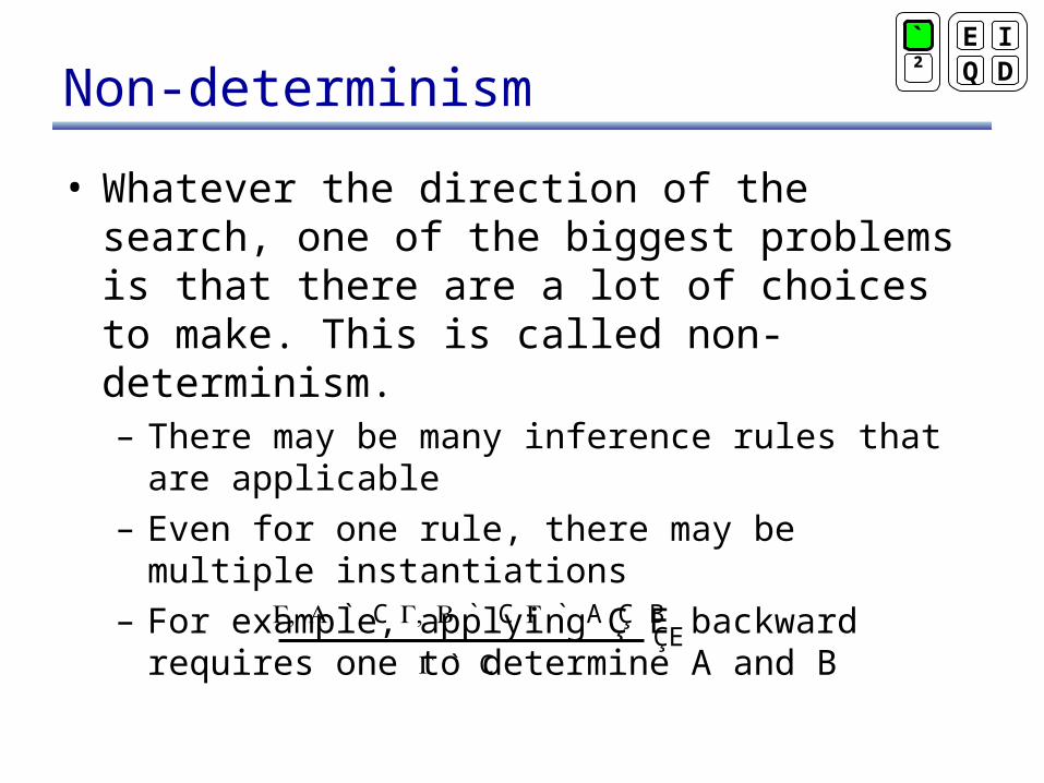
• Whatever the direction of the search, one of the biggest problems is that there are a lot of choices to make. This is called non-determinism.– There may be many inference rules that are
applicable– Even for one rule, there may be multiple instantiations– For example, applying Ç E backward requires one to
determine A and B
`² Q
EDI
` A Ç B
` C ÇE
` C ` C
Two kinds of non-determinism
• Don’t care non-determinism (also called conjunctive non-determinism)– All choices will lead to a successful search, so we
“don’t care” which one we take– Only consideration for making the choice is efficiency
• Don’t know non-determinism (also called disjunctive non-determinism)– Some of the choices will lead to a successful search,
but we “don’t know” which one a priori– In order to deal with this kind of non-determinism, try
all choices using some traversal order (depth-first, breadth-first, iterative deepening
`² Q
EDI

Next lecture
• We’ll see how to reduce non-determinism
• We’ll learn about tactics and tacticals, one of the important techniques used in proof system searches
• We’ll learn about some proof systems that are more suited for automated reasoning, like the sequent calculus and resolution


