Depth to basement with terrestrial gravity for basin-fill aquifer geometry

Case study of Bridgeport Valley, CA

M.S. Thesis Proposal (Hydrogeology)

Elijah T. Mlawsky

elijahmlawsky@gmail.com

Committee:

John N. Louie, Ph.D. – Professor, Primary Adviser, Committee Chair

Greg M. Pohll, Ph.D. – Research Professor, Secondary Adviser (DRI Supervisor)

Alexandra D. Lutz, Ph.D. – Associate Research Professor, Graduate School Representative

November 1, 2015

Abstract:

Basin-fill aquifer characterization is possible with hydrological methods alone, but can

benefit from geophysical depth models. Gravimetric basin depth estimates provide valuable

information on alluvium-buried structure, particularly in regards to boundary fault conditions. By

mapping depth to the basin-bedrock interface, we can infer important geometry constraints on

deep aquifers and boundary controls on principle principal aquifers. Furthermore, basin-scale

terrestrial gravimetry allows flexibility in data point placement; this is meaningful in the study

site of Bridgeport, CA, where a majority of land is privately owned and access to well records

and surface waters is limited. We explore gravity models of the Bridgeport valley, and develop

data point densification strategies to improve model resolution. We propose preliminary depth

estimates of approximately 1275 m at the basin axis center, and suggest further work in the scope

of seismic data correlation, open-source gravity modeling solutions, and in researching the

effects of soil moisture density changes due to seasonal infiltration on gravity findings.

Project Objectives:

Understanding the potential availability of groundwater resources in Eastern California

aquifers is of critical importance to making water management policy decisions and determining

best-use practices for California, as well as for downstream use in Nevada. Hydrologic data can

provide valuable information on aquifer thickness, but is often proprietarily inaccessible or

economically unfeasible to obtain in sufficient quantity. In the case of basin-fill aquifers, it is

possible to make estimates of aquifer geometry from gravity data, constrained by additional

geophysical and geological observations; Lennox and Carlson (1967) long ago demonstrated the

use of gravimetry to map buried valleys and potential aquifers. We design this research to assess

basin thickness about Bridgeport, CA using gravity as the primary metric. In doing so, we

Mlawsky, Elijah 2

circumvent challenges that are associated with hydrologic methods of aquifer characterization,

and demonstrate the utility of a geophysical approach. Ultimately, we look to define basin and

potential aquifer geometry for an area that is not well established in the current knowledge base.

We also test the hypothesis that gravimetric basin studies can provide meaningful insights to

groundwater hydrology with economic feasibility and environmental community benefits over

other characterization methods.

Current hydrological methods involve tomographic pumping tests with well stimulation

and observation of groundwater response at one or more nearby monitoring wells. Saturated

aquifer thickness can be estimated in this manner by way of fitting multiple pump test data with

the unconfined Neuman solution (Maréchal et al. 2010), or alternatively with inverted baseflow

data taken from recession hydrographs (Dewandel et al. 2003). Typically, hydrological methods

for assessing aquifer thickness are the more cost-effective; however, such methods present

challenges when applied to large-scale basin studies. Pumping and streamflow tests often

provide information proximal to wells and channels only, resulting in data of insufficient

resolution for basin depth and range front boundary mapping. Furthermore, tests require access

to said wells, channels, and corresponding records – a particular challenge in the study area of

Bridgeport, CACalifornia, where a majority of land is privately owned and access is proprietary.

Moreover, excavation of new wells for data collection is an invasive procedure and can be

prohibitively expensive.

Geophysical methods are generally less restrictive of basin-scale applications. As shown

by Lennox and Carlson (1967), gravimetry can reveal thickness of permeable deposits of known

density (1967). Additional surveys of electrical resistivity and seismic imaging are used here and

in other common practice to evaluate depth to the basin-bedrock density contrast. As with

Mlawsky, Elijah 3

hydrological methods, geophysical surveys can benefit from unrestricted land access; however,

ease of data point densification along public roads, coupled with 2-dimensional interpolation

provides means of a workaround for potential land access-permission barriers. Survey

deployment and data processing requires minimal training by the methods we delineate below,

thus we estimate low costs of operation beyond the initial equipment purchase. Additionally,

gravimetry and any supporting seismic or potential-field exploration is non-invasive when

compared to methods that involve landscape alteration, noise, or pollutants.

Intellectual Merit:

The existing knowledge base of terrestrial gravity readings for the Eastern Sierras

consists of the Saltus and Jachens dataset compiled for the USGS (1995) and the expanded NSF-

supported dataset at University of Texas, El Paso’s (UTEP) Pan American Center for Earth and

Environmental Studies (PACES; 2015)) (2015). Previously rendered Saltus and Jachens data

results provides a depth model for basins near the California-Nevada border (figure 1) ; (Louie

et al. 2014). While providing a good foundation for this work, the regional scale and data density

prove insufficient for mapping aquifers; we note low resolution of important range-front and

depth features at the single- basin scale about the Bridgeport Valley. Abbot and Louie (2000) and

Widmer et al. (2007) demonstrate the potential for spatial correction by data point densification

on the Reno/Verdi, NV location (figure 2). Here, several hundred new gravity points were

added, resulting in greatly improved definition. Thus, a similar densification effort about

Bridgeport, CA is credible. The PACES dataset is particularly scarce sparse for the Bridgeport

site; there are approximately 800 points within the extent of interest, with poor spatial

distribution – most base dataset points exist outside of the basin, located in the range foothills

and exposed bedrock. We have already improved upon this set by collecting approximately 200

Mlawsky, Elijah 4

new observations in previously scarce sparse areas, and may revisit the field if warranted.

Densification is further motivated by separate Bridgeport basin characterization projects ongoing

by Greg Pohll et al. (2015) and John Louie et al. (2014).

Figure 1: Rendered base dataset of Saltus and Jachens (1995) showing basin thickness. Bridgeport, CA (A) lacks

definition due to data scarcity. Colored traces are Quaternary fault scarps as documented by the USGS (2006).

Figure 2: Densification effects on basin edges and bedrock interface topography for Reno/Verdi, NV. Map (a)

depicts the base dataset, (b) reflects approximately 200 new observations added by Abbot and Louie (2000), and (c)

Mlawsky, Elijah 5

reflects an additional ~200 points from Widmer et al. (2007). Arrows point to important structural information

gained from each addition of data.

The scope of proposed work includes teaching, fieldwork, modeling, and programing

components. These are delineated in the attached timeline. Here, it is important to note that the

proposed methods are both feasible and appropriate for a master’s degree thesis project; i.e., the

task at hand is neither trivial nor impossible to complete in the two years of program study.

Currently, teaching and fieldwork components are complete pending future project direction;

modeling and programming are underway, each with preliminary products available. The

remainder of degree time (approx. one semester) will be spent finalizing deliverables, exploring

product applications, and working on the expanded research goals listed in the future work

section of this proposal.

This project holds additional merit as an interdisciplinary study: geophysical methods

traditionally apply to the fields of seismology and tectonics; though, recent literature depicts a

more prevalent use of geophysics in neighboring fields, such as watershed-scale hydrology

(Robinson et al., 2008). By applying these methods here, we aim to demonstrate the utility and

promote use of geophysics in environmental sciences across many disciplines. We pursue new

outreach opportunities by presenting parts of this research at the 2015 American Geophysical

Union (AGU) conference in San Francisco, as well as actively disseminating research efforts

among peers in the interdisciplinary Graduate Program of Hydrologic Sciences (GPHS). The

methods herein allow for cost and time-efficient estimation of depth to basement and basin-

bedrock interface geometry. By exploring this approach, we hope to draw new insights in a

timeframe that is appropriate for graduate research. We also look for ways of further improving

efficiency of data analysis to promote accessible reproducibility of gravimetric basin depth

methods.

Mlawsky, Elijah 6

Broader Impacts:

The primary motivation for a study of this site stems from work with the Desert Research

Institute (DRI) and its respective client: the National Fish and Wildlife Foundation (NFWF). The

encompassing project is a comprehensive assessment of surface and groundwater reservoirs in

tributary basins for use in conservation planning of the Walker Lake biome. Walker Lake levels

have been in steady decline since 1920, and more information is needed to develop water

management strategies (Pohll 2015). Moreover, there is a need to re-evaluate available

groundwater for California basins, as demonstrated by InSAR data showing significant aquifer

compaction throughout the Antelope Valley (Galloway et al., 1998). Bridgeport remains as an

unknown factor in the extensive water-systems model, largely due to aforementioned land access

issues. A complete basin depth model will benefit the overall study by providing aquifer

boundary information, and may be used by DRI and USGS hydrologists on future ventures.

Deliverables will also lend application to NSF-funded basin study efforts of the Nevada

Seismological Lab and Center for Neotectonic Studies. We collaborate with these groups to

determine formation patterns in Eastern Sierra basins – specifically, geometry at depth. Results

here will benefit Bridgeport and surrounding communities by providing information on seismic

hazards and subsurface structure. These efforts also present educational opportunities: we have

led instruction of geophysical methods on site, teaching survey design and deployment to

University of Nevada, Reno (UNR) undergraduates during a seven-day field course. Students

participated in data acquisition under supervision, and gained direct experience with

contributions to the basin research.

Mlawsky, Elijah 7

Background:

Survey area –

Bridgeport, CA is a tectonic basin located in the northern extent of the Eastern Sierra

Nevada range, 10 miles northwest of Mono Lake. The basin surface encloses approximately 150

km2 of land. The map extent of this study is expanded to approximately 1600 km2, to include

observations of surrounding exposed bedrock. The basin is bounded by distributed normal range-

front faults of the West Walker River fault zone to the northwest, and a series of normal East

Walker River faults to the east (USGS 2006). Glacial ridges close the southern extent of the

basin, and a lateral moraine extends 5 km into the basin past the southern range front at the

ground surface. The East Walker River is the main surface water confluence through the valley,

running north-northwest and exiting though the Bridgeport Reservoir – ultimately terminating at

Walker Lake. Little information is available for the geologic composition for this basin; though,

reports predict shallow Pleistocene glaciations and late Quaternary alluvium fill with region-

typical density of 1.9 – 2.4 g/cm3 (Sharp 1972) (Manger 1963). Saturation favors higher

estimates of fill density; for preliminary models, we use a basin-bedrock density contrast of 0.3

g/cm3 (with bedrock density of 2.67 g/cm3). Ultimately, density uncertainty will affect basin

depth modeling, and should be accounted for by creating a range of outputs corresponding to

various mean fill densities. The Saltus and Jachens data suggests basin depth of roughly 1 – 2 km

in neighboring basins, using the above density contrast.

Mlawsky, Elijah 8

Theory and case studies –

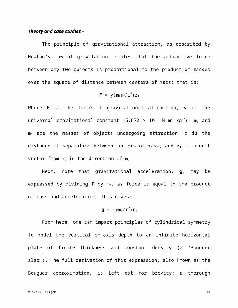
The principle of gravitational attraction, as described by Newton’s law of gravitation,

states that the attractive force between any two objects is proportional to the product of masses

over the square of distance between centers of mass; that is:

F = γ(m1m2/r2)r1

Where F is the force of gravitational attraction, γ is the universal gravitational constant (6.672 ×

10-11 N m2 kg-2), m1 and m2 are the masses of objects undergoing attraction, r is the distance of

separation between centers of mass, and r1 is a unit vector from m2 in the direction of m1.

Next, note that gravitational acceleration, g, may be expressed by dividing F by m2, as

force is equal to the product of mass and acceleration. This gives:

g = (γm1/r2)r1

From here, one can impart principles of cylindrical symmetry to model the vertical on-

axis depth to an infinite horizontal plate of finite thickness and constant density (a “Bouguer

slab”). The full derivation of this expression, also known as the Bouguer approximation, is left

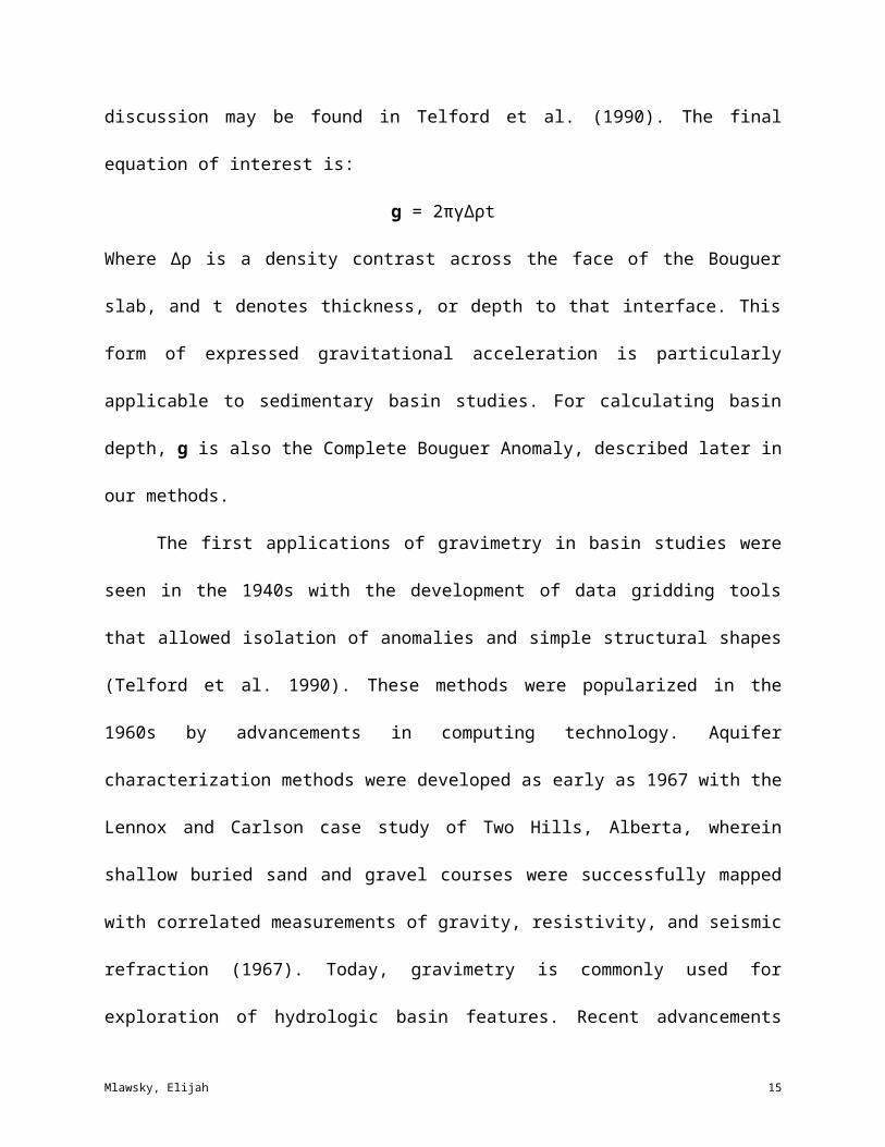
out for brevity; a thorough discussion may be found in Telford et al. (1990). The final equation

of interest is:

g = 2πγ∆ρt

Where ∆ρ is a density contrast across the face of the Bouguer slab, and t denotes thickness, or

depth to that interface. This form of expressed gravitational acceleration is particularly

applicable to sedimentary basin studies. For calculating basin depth, g is also the Complete

Bouguer Anomaly, described later in our methods.

The first applications of gravimetry in basin studies were seen in the 1940s with the

development of data gridding tools that allowed isolation of anomalies and simple structural

Mlawsky, Elijah 9

shapes (Telford et al. 1990). These methods were popularized in the 1960s by advancements in

computing technology. Aquifer characterization methods were developed as early as 1967 with

the Lennox and Carlson case study of Two Hills, Alberta, wherein shallow buried sand and

gravel courses were successfully mapped with correlated measurements of gravity, resistivity,

and seismic refraction (1967). Today, gravimetry is commonly used for exploration of

hydrologic basin features. Recent advancements have been made in the area of gridding and

isolation: Jachens and Moring improved on basin thickness determination methods by

developing the procedure of classifying data points by basin or bedrock surface composition and

assigning class densities (1990). This allows separate gridding of anomaly trends for different

compositions (basin and bedrock) and grid subtraction for a detailed residual map of isolated

basin-fill gravity. Furthermore, work by Abbott and Louie demonstrates successful

implementation of these residual gridding methods in other basins about the Eastern Sierras

(2000).

Geophysical survey methods are often categorized as either integral or derivative.

Integral methods, also referred to as natural-source or potential field methods, are those that

provide structural information over an area by fitting a non-unique solution to the data. That is to

say, an infinite number of modeled density distributions may fit a gravity model, and it is up to

the modeler to make logical interpretations. Integral methods include gravimetry, magnetometry,

and some electrical surveys among others. These are apt for large-scale model applications

where it is necessary to interpolate a potential surface across measured points. Derivative

methods provide numerical models that are forward in time and space, and by contrast are better

suited for creating detailed structural profiles along a survey transect. Derivative methods are

largely considered more accurate, though less cost and time-efficient (Telford et al. 1990).

Mlawsky, Elijah 10

Gravimetry has the benefits of rapid deployment, large coverage, and low operational costs;

however, lacks accuracy when compared to a derivative method, such as seismic imaging.

Ideally, gravity models are constrained by supplemental data – be that from a correlated

derivative survey or additional integral survey.

Cross-correlation of derivative or additional integral methods with gravimetry is an

effective means of reducing uncertainties; gravimetry is a proven tool for estimating basin-scale

geometry, but can present challenges when used as the sole interpretation basis for detailed

structure (e.g. specific geometry of seismic networks). Such is the case in Kostoglodv et al.

where regional fault slopes are determined by assessing the trend in Bouguer anomalies, and

abrupt changes in dip angles became apparent under seismic investigation (1996). Comparison of

the methods showed strong correlation of the inferred location of faults and subducted slabs,

reaffirming interpretations. Correlative surveys are potentially important to the Bridgeport study,

as faults can act as barriers to groundwater flow, and may therefore interest other modelers

working on the Walker Lake system model. If time and resources allow, deploying a passive

seismic micro-tremor survey across prominent fault scarps may help to establish a more detailed

interpretation of underlying structure. This item should be considered after addressing the

immediate project goals discussed under results and future work.

Methods:

Data acquisition –

Three sources of gravity data constitute model inputs: fully processed CBA data made

publically available by PACES, UTEP; raw gravity data collected about the Bodie Hills, CA and

shared with permission by Dr. Richard Blakely and Chad Carlson (John et al. 2012); and newly

collected data throughout the Bridgeport Valley. The placement of new observation points is

Mlawsky, Elijah 11

influenced by several factors, primarily land access (public v. private), existing data point

density, and location of potential boundary faults listed in the USGS Qfaults database (2006).

We collect new data in lines containing 5-10 observation points each, with observation nodes

spaced at roughly 200 m. In-line collection allows forward modeling of profiles to resolve sub-

basin scale features, such as fault form at depth, which are vital to defining lateral boundaries of

the basin. Below, figure 3 depicts all current gravity observation points, or “base stations,”

color-grouped by source.

{FIGURE 3 PLACEHOLDER}

In constructing the basin model, we incorporate many gravity observations: 818 are

extracted from the PACES database, 67 from Blakely and Carlson, and 134 are original

observations. We regard these collectively as a bulk dataset, as the data therein are compiled

from multiple sources. Inconsistencies among source instrumentation and processing can result

in “static offsets,” or artificial bull’s-eye contours within the gravity gradient. Amending suspect

offsets is a time-consuming process when modeling large-scale basin features. To maintain

efficient workflow, we developed a MATLAB script for interpolating the CBA contour across

the basin using sparse observation points, and leveling offsets to the datum with user-defined

sensitivity. The script is also capable of plotting gravity profiles between any two points on the

map extent – a useful feature for end-user deliverables. The resulting anomaly map provides an

efficient means of locating and removing static offsets in the data, while also providing a fast

visual representation of the bulk dataset. Further development could end in a more accessible

alternative to the proprietary modeling tools used in the modeling process; however, the use of

MATLAB for more than the removal of offsets is beyond the immediate scope of these methods.

Mlawsky, Elijah 12

We revisit applications of non-proprietary modeling platforms in our forthcoming AGU abstract

and in the future work section of this proposal.

The goal of data point densification is to increase the number of nodes that an

interpolation surface can fit, thereby increasing the accuracy of interpolated data between

measured points. Past work by Saltus and Jachens, Abbott and Louie, and Widmer et al. (1995;

2000; 2007) demonstrates the effectiveness of densification on the base dataset. Boundary

densification in Bridgeport means accessing points in remote areas, often over challenging

terrain. Collecting new data there requires only proper safety and determination, whereas data

acquisition on privately owned lands often presents the greater barrier. Land ownership is an

item of consideration in Bridgeport, as estimates indicate upwards of 75% of basin land is

designated as privately owned. Throughout this study, we continue to work with Mono County

officials and local stakeholders to promote awareness of research objectives and to establish

rapport with private landowners. Efforts thus far have resulted in generous access to survey

private land within the Hunewill Ranch – a 26,000-acre parcel at the southwest of the valley,

yielding approximately one-third of the new observations. Despite continued efforts, many other

valley stakeholders remain hesitant to allow survey access. We can resolve data gaps over

private land by initializing survey lines at property bounds, and extending them over public land

outward toward the range fronts. This results in a survey line on which interpolation can best

project gravity gradients into the valley center, or other off-limit areas. This solution is less ideal

than having real data on ranch lands, but does provide a workable substitute.

We record new observations with a Lacoste and Romberg (L&R) G-509 gravimeter

(accurate to 0.1 mGal), with relative elevation control (accurate to 0.3 m) obtained through a

Trimble R10 RTX geodetic GPS unit. Vertical GPS precision lends to increased accuracy in

Mlawsky, Elijah 13

processing terrain corrections. We measure gravity at an established control point at the

beginning and end of each workday for use in calculating mechanical instrument drift. Similarly,

we establish “loop closure” by re-recording the first observation point of a line every two hours.

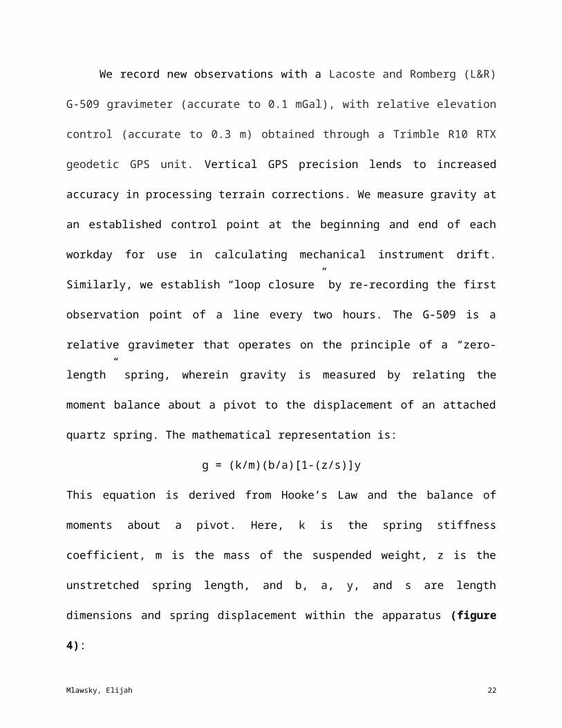
The G-509 is a relative gravimeter that operates on the principle of a “zero-length” spring,

wherein gravity is measured by relating the moment balance about a pivot to the displacement of

an attached quartz spring. The mathematical representation is:

g = (k/m)(b/a)[1-(z/s)]y

This equation is derived from Hooke’s Law and the balance of moments about a pivot. Here, k is

the spring stiffness coefficient, m is the mass of the suspended weight, z is the unstretched spring

length, and b, a, y, and s are length dimensions and spring displacement within the apparatus

(figure 4):

Figure 4: Schematic of a zero-length spring apparatus, used in the L&R relative gravimeter (University of

Oklahoma 2015).

Most terrestrial gravimeters provide relative measurements; that is, measurements do not

reflect the actual gravitational acceleration at the observation point. Absolute gravity is

Mlawsky, Elijah 14

determined with an optical laser interferometer, which measures the free-fall acceleration of a

retroreflector in a vacuum. Conversion of relative measurements to absolute gravity is necessary

for calculations and is accomplished by recording a relative measurement at a location with

known absolute gravity and obtaining a scale factor.

Data processing –

Raw data are transcribed to .csv files, separated by date and line for processing. We

correct for instrument drift, tidal effects, and terrain contributions using QCTool software.

Terrain corrections use the Global 30 Arc-Second (GTOPO30) digital elevation model (DEM)

available from the US Geological Survey. We discern local from regional terrain effects by the

Hammer method (1939), with an inner-ring (local terrain) radius of 1000 m and outer-ring

(regional terrain) calculated to the recommended Bullard B limit of 166 km or 1.5° (Nowell

1999). After applying corrections to the raw observation, we find absolute gravity at each base

station using a scale factor determined by comparing relative measurements to an established

absolute measurement located on the UNR campus (Jablonksi 1974). Then, we calculate latitude

effects, Free Air (0.308596 mGal/m), and Bouguer components in accordance with the North

American standards (Hinze et al. 2005). The Complete Bouguer Anomaly (CBA) is the resulting

difference of corrected absolute gravity, latitudinal, Free Air, and Bouguer components, added

with terrain corrections.

Once processed, CBA data is added to the existing gravity framework and then gridded to

50 m cell spacing. The resulting CBA grid is sparse, in that it contains data only near known

observation points. We resolve unknowns with a minimum-curvature, or least-squares-fit,

interpolation algorithm in Oasis montaj, across a map extent that encompasses the basin and

contributing local terrain. We then remove bedrock gravity to isolate basin gravity anomalies: for

Mlawsky, Elijah 15

preliminary results, the data inversion was accomplished with a simplified linear trend removal

of bedrock gravity; finalized products will use the Jachens and Moring method of point

classification and grid subtraction.

The obtained residual grid of isolated basin gravity allows conversion to basement depth

by the infinite Bouguer slab approximation. Aquifer-geometry estimates draw upon this newly

defined basin-floor topography and the existing knowledge base of local tectonics, i.e. basin-

bounding faults. Results could benefit by constraining aquifer models with additional

geophysical and geological observations. We predict that the porosity of basin-fill materials

decreases with depth due to compaction in the manner described by Athy (1930). Thereupon,

lateral boundary definition, or basement convergence, is of particular importance in defining the

storage capacity of the aquifer.

Preliminary Results and Future Work:

Figure 5 shows the basin depth, reflecting data as of August 2015. Approximately 30

additional observations have been collected along the northeastern side of the basin since the

drafting of this figure. The map scale is redacted due to software error; this is easily amendable

once modeling software is back online. The depth scale and relative spatial distribution,

however, are accurate. A full discussion and interpretation of results is reserved for the final end

products. Here, we note a preliminary basin depth of 1275 m. This is in reasonable agreement

with proximal Eastern Sierra basins (figure 1, above). Immediate next steps will focus on

implementing a Jachens and Moring-style residual grid for all data to date, generating a control

map of the PACES base dataset, and creating forward models of important boundary structure

and basin profiles.

Mlawsky, Elijah 16

Figure 5: Preliminary depth to the basin-bedrock interface for Bridgeport, CA, with a minimum curvature fitting

algorithm, density contrast of 0.3 g/cm3, and grid cell spacing of 50 m. Map scale redacted due to coordinate

conversion error; depth scale is accurateas intended.

Therefore, the end products of research will include: a full depth to basement map of the

Bridgeport basin, geospatial files for client visualization (ArcGIS or Google Earth maps with

overlays for topology, geology, land-use, etc.), forward-modeled profiles of interest, and a

control model of PACES-only data for measuring the effects of densification. Efforts will also be

Mlawsky, Elijah 17

made to quantify the costs of densification. Model evaluation remains a difficult step in the

overall process – with limited geological information for the Bridgeport area, we will test

validity by comparing end results to known depths for proximal basins of similar age and origin.

In addition to thoughts on incorporating correlative methods (above), we address ideas

for potential future work here:

Soil moisture simulations –

Further interdisciplinary research efforts can also benefit result accuracy: while post-

processing of gravity data accounts for variables such as tide, instrument drift, and terrain, the

corrections do not capture the effects of a dynamic water system. By modeling simulations of

precipitation and evapotranspiration, we can gauge the density added to vadose soils by water

infiltration. Thus, we can gain a new gravity correction for rainfall events as a function of event

size, vegetation coverage, and elapsed time. The infiltration amount with residence time is first

calculated using the unsaturated flow model, HYDRUS; we can then extract a basin density

change and convert to gravity with the Bouguer slab approximation. We then apply this

correction to observations collected during or shortly after precipitation, if determined to be a

significant control. In doing so, we reduce uncertainties in the basin density and thereby depth,

and are better able to assimilate data collected under various weather conditions.

Open-source modeling platforms –

The majority of post-processing for this work has implemented proprietary gravimetry

modeling packages, namely Oasis montaj and QC Tool. While both platforms provide excellent

gravity modeling capabilities, licensing restrictions can limit the reproducibility of these

methods. Moreover, limited access to proprietary software resources has slowed workflow on

this project. There is a clear need for an open-source solution to simple gravity corrections and

Mlawsky, Elijah 18

mapping. If pursuing this goal, we will draw upon the MATLAB mapping and profiling script

(discussed above), converting existing visualization functionality to the Python language. We

would then need to program means of corrections and residual grid formation. The resulting

program would be simple in design, and may have additional utility in gravity modeling

education.

Timeline:

We list important project milestones by semester with a two-year anticipated timeframe.

The funding source is noted, as project efforts can accommodate the interests of each sponsor

while maintaining an overall focus on answering the primary research question. Completed tasks

are preceded by a checked box symbol, . Boldfaced items are those copied directly from the

GPHS student handbook, M.S. degree checklist (2014).

First semester - Fall 2014, funding: TA (UNR, Ecohydrology)

Upon arriving at the University schedule an appointment with the Program Director

for an entrance interview. At this meeting you will be asked to complete a Student

Information Form and an Initial Advisement Worksheet.

Attend the New Graduate Student Orientation that assists graduate students in

familiarizing themselves with the university and its support services. It is a required

program for all new graduate students.

During the first year of study you should develop a research proposal in concert with

your advisor.

Second semester - Spring 2015, funding: GRA (DRI/NFWF; Pohll)

Mlawsky, Elijah 19

In consultation with your advisor establish an academic committee. The committee

must contain at least three members, including your advisor, and at least one committee

member who is from outside of your home department.

Draft methods proposal for DRI/NFWF.

Begin fieldwork; lead one-week field instruction in Bridgeport, CA and demonstrate applied

geophysical methods in gravity, geodetic GPS, and magnetics to undergraduate class.

Become familiar with modeling software packages: Oasis montaj, QC Tool, and MATLAB.

Post-process gravity data and begin background research.

Summer semester - Fall 2015, funding: GRA (DRI/NFWF; Pohll)

Attend two-week modeling course in Boise, ID. Develop understanding of modeling

practices, applications, and ethics.

Continue to gather and post-process new gravity data about Bridgeport, CA.

Model preliminary results and discuss with DRI supervisor, Greg Pohll.

Third semester - Fall 2015, funding: GRA (DRI/NFWF; Pohll)

Prior to the first committee meeting, complete the Program of Study Document (see

http://www.unr.edu/grad/forms). Bring this document to the Program Director for

review. Please review the Graduate Program of Hydrologic Sciences Planning Guide

and the Graduate School Catalog to ensure that your coursework fulfills both the

Program and Graduate School requirements.

☐ Once your advisor approves the research proposal, distribute it to your committee two

weeks prior to the first committee meeting. It is the student’s responsibility to schedule

the committee meeting.

Mlawsky, Elijah 20

☐ Make an oral presentation of your research proposal to the academic committee and

gain committee approval to proceed. Your committee should review, approve and sign

your Program of Study Document. If all committee signatures are in place, the

Program Director will sign the document and deliver it to the Graduate School.

Program of Study deadline: third week of NOVEMBER for MAY graduation.

☐ Attend AGU from December 14-18, 2015. Present non-traditional gravity modeling methods

using MATLAB for hydrologic basin studies. Receive professional feedback on project-to-

date.

Fourth semester - Spring 2016, funding: GRA (UNR/NSF; Louie, Wesnousky, Faulds)

☐ Consult with Center for Neotectonic Studies; use results to interpret formation processes.

Gather additional gravity data at boundary faults if needed.

☐ Explore soil moisture models and test significance of infiltrated waters on density following

precipitation events.

☐ Perform additional assessments (Economic analysis, error assessments, etc.).

☐ Complete your Application for Graduation document and obtain your advisor’s

signature. Deliver the application to the Program Director for his/her signature and

delivery to the Graduate School. The application is available online at:

http://www.unr.edu/grad/forms. Graduation application deadline: MARCH 1 for MAY

graduation.

☐ Prepare a draft of your thesis or professional paper and obtain advisor approval.

Distribute the approved and complete document to your committee at least two weeks

prior to the defense date. It is the responsibility of the student to schedule the defense

date and location. Send the Program Director (hydro@unr.edu) an announcement of

Mlawsky, Elijah 21

the defense with the date, time, location, and thesis title at least one week prior to the

defense date. If the defense is not announced at least one week prior to the defense date,

the Program Director will not sign your Notification of Completion Document and you

will have to reschedule.

☐ Make an oral presentation (Defense) of your thesis or professional paper to the

academic committee and gain committee approval to graduate. (MAY 2016)

☐ Make final corrections to your thesis or professional paper and then complete your

Notification of Completion Document (see http://www.unr.edu/grad/forms) and obtain

committee signatures. Obtain the Program Director’s signature, and then deliver to the

Graduate School. Follow the instructions on the Thesis/Dissertation guidelines and

submission requirements (see http://www.unr.edu/grad/forms/thesis-filing- guidelines)

to file your thesis. The signed copy of your Notice of Completion must be submitted to

the Graduate School approximately two weeks before the official end of the semester

(see http://www.unr.edu/grad/graduation-and- deadlines for the actual dates).

Mlawsky, Elijah 22

Works Cited

Abbott, Robert E, and John N Louie. 2000. “Depth to Bedrock Using Gravimetry in the Reno and Carson City, Nevada, Area Basins.” Geophysics 65 (2): 340–50.

Athy, L. F. 1930. “Density, Porosity, and Compaction of Sedimentary Rocks.” AAPG Bulletin 14 (1): 1–24.

Dewandel, B, P Lachassagne, M Bakalowicz, Ph Weng, and A Al-Malki. 2003. “Evaluation of Aquifer Thickness by Analysing Recession Hydrographs. Application to the Oman Ophiolite Hard-Rock Aquifer.” Journal of Hydrology 274 (1–4): 248–69. doi:10.1016/S0022-1694(02)00418-3.

Galloway, D. L., K. W. Hudnut, S. E. Ingebritsen, S. P. Phillips, G. Peltzer, F. Rogez, and P. A. Rosen. 1998. “Detection of Aquifer System Compaction and Land Subsidence Using Interferometric Synthetic Aperture Radar, Antelope Valley, Mojave Desert, California.” Water Resources Research 34 (10): 2573–85. doi:10.1029/98WR01285.

“Graduate Program of Hydrologic Sciences Student Handbook.” 2014. University of Nevada, Reno. http://www.cabnr.unr.edu/saito/gphs_handbook.htm.

“Gravity Database of the US.” 2015. Univeristy of Texas, El Paso Pan American Center for Earth and Environmental Studies.

Hammer, S. 1939. “Terrain Corrections for Gravimeter Stations.” GEOPHYSICS 4 (3): 184–94. doi:10.1190/1.1440495.

Hinze, William J., Carlos Aiken, John Brozena, Bernard Coakley, David Dater, Guy Flanagan, René Forsberg, et al. 2005. “New Standards for Reducing Gravity Data: The North American Gravity Database.” Geophysics 70 (4): J25–32. doi:10.1190/1.1988183.

Jablonksi, H. M. 1974. “World Relative Gravity Reference Network North America, Parts 1 and 2: U.S. Defense Mapping Agency Aerospace Center Reference.”

Jachens, R.C., and B.C. Moring. 1990. “Maps of the Thickness of Cenozoic Deposits and the Isostatic Residual Gravity over Basement for Nevada.” USGS Numbered Series 90-404. Open-File Report. U.S. Dept. of the Interior, Geological Survey,. http://pubs.er.usgs.gov/publication/ofr90404.

John, David A., Edward A. du Bray, Richard J. Blakely, Robert J. Fleck, Peter G. Vikre, Stephen E. Box, and Barry C. Moring. 2012. “Miocene Magmatism in the Bodie Hills Volcanic Field, California and Nevada: A Long-Lived Eruptive Center in the Southern Segment of the Ancestral Cascades Arc.” Geosphere 8 (1): 44–97. doi:10.1130/GES00674.1.

Kostoglodov, V., W. Bandy, J. Domínguez, and M. Mena. 1996. “Gravity and Seismicity over the Guerrero Seismic Gap, Mexico.” Geophysical Research Letters 23 (23): 3385–88. doi:10.1029/96GL03159.

Lennox, DH, and V Carlson. 1967. “Geophysical Exploration for Buried Valleys in an Area North of Two Hills, Alberta.” Geophysics 32 (2): 331–62.

Louie, John, Steven Wesnousky, and James Faulds. 2014. “Proposal for Walker Lane Shear Zone Invesitgation.”

Manger, Edward. 1963. “Porosity and Bulk Density of Sedimentary Rocks.” US Geological Survey.

Maréchal, Jean-Christophe, Jean-Michel Vouillamoz, M. S. Mohan Kumar, and Benoit Dewandel. 2010. “Estimating Aquifer Thickness Using Multiple Pumping Tests.” Hydrogeology Journal 18 (8): 1787–96. doi:10.1007/s10040-010-0664-3.

Mlawsky, Elijah 23

“Measuring Gravity: Relative Measurements.” 2015. Accessed November 4. http://principles.ou.edu/grav_ex/relative.htm.

Nowell, D. A. G. 1999. “Gravity Terrain Corrections — an Overview.” Journal of Applied Geophysics 42 (2): 117–34. doi:10.1016/S0926-9851(99)00028-2.

Pohll, Greg. 2015. “Hydrologic Modeling Tools for the Upper Walker River Basin.” presented at the Graduate Program of Hydrologic Sciences Colloquium, University of Nevada, Reno, March.

“Quaternary Fault and Fold Database for the United States.” 2006. .kmz. US Geological Survey. http://earthquake.usgs.gov/hazards/qfaults/.

Robinson, D. A., A. Binley, N. Crook, F. D. Day-Lewis, T. P. A. Ferre, V. J. S. Grauch, R. Knight, et al. 2008. “Advancing Process-Based Watershed Hydrological Research Using near-Surface Geophysics: A Vision For, and Review Of, Electrical and Magnetic Geophysical Methods.” Hydrological Processes 22 (18): 3604–35. doi:10.1002/hyp.6963.

Saltus, Richard W, and Robert C Jachens. 1995. Gravity and Basin-Depth Maps of the Basin and Range Province, Western United States. US Geological Survey.

Sharp, Robert P. 1972. “Pleistocene Glaciation, Bridgeport Basin, California.” Geological Society of America Bulletin 83 (8): 2233–60. doi:10.1130/0016-7606(1972)83[2233:PGBBC]2.0.CO;2.

Telford, William Murray, W. M. Telford, L. P. Geldart, and Robert E. Sheriff. 1990. Applied Geophysics. Cambridge University Press.

Widmer, M.C., P.H. Cashman, F.C. Benedict, and J.H. Trexler. 2007. “Neogene Through Quaternary Stratigraphy And Structure In A Portion Of The Truckee Meadows Basin: A Record Of Recent Tectonic History.” In . https://gsa.confex.com/gsa/2007CD/finalprogram/abstract_121055.htm.

Mlawsky, Elijah 24