3 Crisis Management in Capital Markets: The Impact of Argentine Policy during the Tequila Effect Eduardo J. J. Ganapolsky and Sergio L. Schmukler Abstract The Mexican financial crisis of 1994–95 had strong spillover effects on Argen- tina. The Argentine government successfully announced a series of policies to mitigate the contagion effects. This article studies how capital markets reacted to each policy announcement and news reports. Capital markets welcomed announcements that demonstrated a firm commitment to the currency board. The agreement with the International Monetary Fund (IMF), the dollarization of reserve deposits in the central bank, and changes in reserve requirements had a strong positive impact on market returns. After a period of higher vola- tility, the appointment of a new finance minister significantly decreased the variance of stock and bond returns, while lower reserve requirements increased the volatility of interest rates. The financial crises that began in Mexico (1994) and in Thailand (1997) had strong spillover effects on other countries. The Mexican crisis af- fected, among others, Argentina and Brazil, as well as Malaysia, the Philippines, and Thailand. The forced flotation of the Thai baht prompted devaluations in Indonesia, Malaysia, the Philippines, and the Republic of Korea, while it provoked a much wider direct or indirect turbulence in both developed and emerging markets around the world. The global extent of recent crises and the potential damaging conse- quences of being affected by contagion continue to attract attention among economists and policymakers. Most of the research concentrates
Transcript
3
Crisis Management in Capital Markets:The Impact of Argentine Policy
during the Tequila Effect
Eduardo J. J. Ganapolsky and Sergio L. Schmukler
Abstract
The Mexican financial crisis of 1994–95 had strong spillover effects on Argen-tina. The Argentine government successfully announced a series of policies tomitigate the contagion effects. This article studies how capital markets reactedto each policy announcement and news reports. Capital markets welcomedannouncements that demonstrated a firm commitment to the currency board.The agreement with the International Monetary Fund (IMF), the dollarizationof reserve deposits in the central bank, and changes in reserve requirementshad a strong positive impact on market returns. After a period of higher vola-tility, the appointment of a new finance minister significantly decreased thevariance of stock and bond returns, while lower reserve requirements increasedthe volatility of interest rates.
The financial crises that began in Mexico (1994) and in Thailand (1997)had strong spillover effects on other countries. The Mexican crisis af-fected, among others, Argentina and Brazil, as well as Malaysia, thePhilippines, and Thailand. The forced flotation of the Thai bahtprompted devaluations in Indonesia, Malaysia, the Philippines, and theRepublic of Korea, while it provoked a much wider direct or indirectturbulence in both developed and emerging markets around the world.
The global extent of recent crises and the potential damaging conse-quences of being affected by contagion continue to attract attentionamong economists and policymakers. Most of the research concentrates
4 Eduardo J. J. Ganapolsky and Sergio L. Schmukler
on understanding the causes and consequences of financial crises. Inthis article, we focus on another aspect of financial crises: how crisismanagement might change the dynamics of contagion or spillover ef-fects. Once a country has been affected by the spillover effects of anexternal crisis, what policies help resolve a crisis? On the other hand,what kinds of announcements and news events negatively impact capi-tal markets?1
During the recent Mexican and Asian crises, several approaches weretried to avert the spillover effects. For instance, in the case of the Mexi-can crisis, Argentina’s former finance minister wanted to change themarkets’ expectations by showing a strong commitment to defendingthe exchange rate peg. On March 11, 1995, The Economist reported thefollowing:
Mr. Cavallo has said that he would rather “dollarize” theeconomy entirely than devalue the peso.
While Argentina tried to reinforce the free convertibility of its currencyduring the Mexican crisis, Malaysia attempted to insulate its financialmarkets from speculative pressure during the Asian crisis. Accusingforeign speculators of orchestrating Malaysia’s economic crisis, Malay-sian Prime Minister Mahathir Mohamad (New York Times, September21, 1997) said the following:
Currency trading is unnecessary, unproductive and totallyimmoral. It should be made illegal.
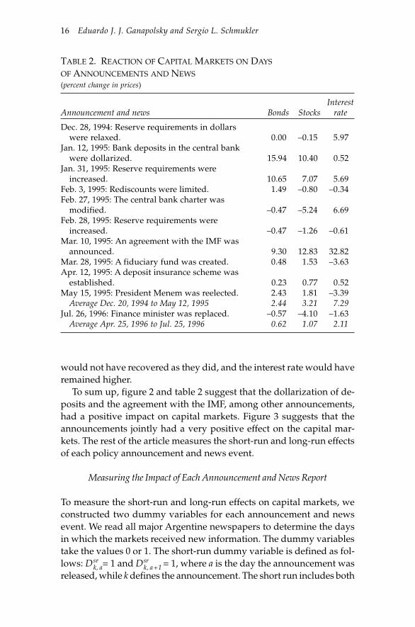
In this article we analyze the experience of Argentina during thespillover of the Mexican crisis, dubbed the “tequila effect.” Argentinapresented an excellent opportunity to study crisis management. First,Argentina was arguably the country most affected by the Mexican pesodevaluation on December 20, 1994, besides Mexico itself. Argentina’speg to the dollar and overall financial stability were reexamined duringthe tequila effect. On December 28 the central bank sold $353 million ofreserves (the largest amount since the currency board was established).In the three months following the Mexican peso devaluation, the cen-tral bank sold more than one-third of its foreign exchange reserves.
1. In this article, “announcements” refer to policy measures undertaken bythe government, like signing an agreement with the international financial com-munity. “News” events refer to meaningful economic or political episodes—like a presidential election or the appointment of a new finance minister.
CRISIS MANAGEMENT IN CAPITAL MARKETS 5
Argentina’s stock market index plummeted 50 percent between Decem-ber 19, 1994, and March 8, 1995. Argentine bond prices fell 36 percent,and the peso interest rate jumped from 11 percent to 19 percent duringthe same period. By March 11, 1995, there was great uncertainty aboutArgentina’s fortunes, and The Economist reported:
The big question to the [Latin American] region is whetherrecession will force the Argentines to . . . devalue.
Second, Argentina is under a currency board system, which constrainsits monetary policy. At least 80 percent of the monetary base had to bebacked by U.S. dollar reserves or other internationally liquid assets (notissued by the Argentine government).2 Dollar-denominated bonds issuedby the Argentine government can back the rest of the monetary base.Therefore, Argentina’s policymakers needed to use alternative instru-ments, other than monetary policy, to revert the negative external shock.
Third, Argentina’s policymakers took an active role in preventing afinancial crash and a devaluation of the peso. Finally, Argentina wassuccessful in controlling the negative transmission. During the Asianand Russian crises, Argentina’s expertise in dealing with crises had al-ready been internationally acknowledged. The financial press reportssome examples:
Argentines have an excellent experience in crisis manage-ment . . . Thailand should talk to them.
William Rhodes, vice president of Citibank,La Nación (newspaper), September 23, 1997
It was kind of strange to come from Latin America [to Asia]and try to give some advice, because for years it was thereverse.
Miguel Kiguel, Argentina’s finance undersecretary,Dow Jones International, September 23, 1997
Cavallo steps in to advise Moscow.
Financial Times, August 31, 1998
2. In 1995 more than 80 percent of the monetary base was backed by inter-national assets. The Convertibility Law allows international reserves to be atleast two-thirds of the monetary base.
6 Eduardo J. J. Ganapolsky and Sergio L. Schmukler
In this article, we study Argentina’s crisis management by analyzinghow different policy announcements and news affected Argentina’sstock market index, Brady bond prices, and peso-deposit interest rates.Among the announcements and news received by the markets, we foundthe following: The central bank lowered reserve requirements—on U.S.dollar deposits and on peso deposits—to assist troubled institutions andto reactivate the economy. Peso deposits in the central bank were auto-matically converted into U.S. dollars to give reassurance to the currencyboard. Rediscounts were limited. The central bank charter was reformedto gain more flexibility to act as a lender of last resort. An agreementwith the IMF was reached. A fiduciary fund for bank capitalization wasissued to support weak institutions, and a deposit insurance was estab-lished. Finally, President Menem was reelected, and the finance minis-ter was replaced.
The remainder of the article is organized as follows. The next sec-tion, “Crisis Management under Contagion,” describes in detail the an-nouncements and news received by the markets. The following section,“Short-Run and Long-Run Impact of Policy Announcements and News,”studies how each announcement and news report affected the short-run and long-run returns of financial variables. The penultimate section,“The Impact of Announcements and News on Volatility,” focuses onhow announcements and news impacted the markets’ volatility. Finally,the last section summarizes the results and concludes the discussion.
Crisis Management under Contagion
Latin American capital markets have become increasingly integratedamong themselves and with the rest of the world. Asset prices fromdifferent countries tend to co-move, so an external shock, such as theMexican one, is transmitted to other countries. The high correlation ofasset prices between Argentina and Mexico makes Argentina particu-larly sensitive to changes in Mexican prices. Many papers have arguedthat markets are prone to “contagion.”3 For instance, Calvo and Reinhart
3. “Contagion” has been defined differently across papers. At one extreme,“contagion” is understood as the spillover of shocks across countries. At theother end, under a more restrictive definition, “contagion” means the trans-mission of shocks unrelated to “market fundamentals.” The evidence broadlysuggests that there was contagion, in the restrictive sense, from Mexico toArgentina in 1994–95.
CRISIS MANAGEMENT IN CAPITAL MARKETS 7
(1996), Valdés (1996), Baig and Goldfajn (1998), Frankel and Schmukler(1998), and Ganapolsky and Schmukler (1998) study the presence of“excess co-movement” between Argentina and Mexico, among othercountries. Using a different approach, Eichengreen, Rose, and Wyplosz(1996) and Kaminsky and Reinhart (2000) study contagion by testingwhether the probability of a crisis increases when there is a crisis some-where else. Given the spillover effects from Mexico to Argentina, thepresent article studies the impact of the Argentine policy response tothe contagion that originated in Mexico.
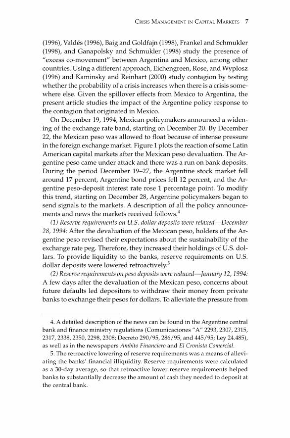
On December 19, 1994, Mexican policymakers announced a widen-ing of the exchange rate band, starting on December 20. By December22, the Mexican peso was allowed to float because of intense pressurein the foreign exchange market. Figure 1 plots the reaction of some LatinAmerican capital markets after the Mexican peso devaluation. The Ar-gentine peso came under attack and there was a run on bank deposits.During the period December 19–27, the Argentine stock market fellaround 17 percent, Argentine bond prices fell 12 percent, and the Ar-gentine peso-deposit interest rate rose 1 percentage point. To modifythis trend, starting on December 28, Argentine policymakers began tosend signals to the markets. A description of all the policy announce-ments and news the markets received follows.4
(1) Reserve requirements on U.S. dollar deposits were relaxed—December28, 1994: After the devaluation of the Mexican peso, holders of the Ar-gentine peso revised their expectations about the sustainability of theexchange rate peg. Therefore, they increased their holdings of U.S. dol-lars. To provide liquidity to the banks, reserve requirements on U.S.dollar deposits were lowered retroactively.5
(2) Reserve requirements on peso deposits were reduced—January 12, 1994:A few days after the devaluation of the Mexican peso, concerns aboutfuture defaults led depositors to withdraw their money from privatebanks to exchange their pesos for dollars. To alleviate the pressure from
4. A detailed description of the news can be found in the Argentine centralbank and finance ministry regulations (Comunicaciones “A” 2293, 2307, 2315,2317, 2338, 2350, 2298, 2308; Decreto 290/95, 286/95, and 445/95; Ley 24.485),as well as in the newspapers Ambito Financiero and El Cronista Comercial.
5. The retroactive lowering of reserve requirements was a means of allevi-ating the banks’ financial illiquidity. Reserve requirements were calculatedas a 30-day average, so that retroactive lower reserve requirements helpedbanks to substantially decrease the amount of cash they needed to deposit atthe central bank.
8 Eduardo J. J. Ganapolsky and Sergio L. Schmukler
FIGURE 1. EVOLUTION OF INTERNATIONAL CAPITAL MARKETS DURING THE MEXICAN CRISIS
(all markets equal 100 on December 20, 1994)
Dollars130120110100
90807060504030Dec. 1,
1994
U.S.
Mexico
Stock markets
Dec. 30,1994
Jan. 30,1995
Feb. 28,1995
Mar. 29,1995
Apr. 27,1995
May 26,1995
Chile
Argentina
Brazil
Dollars120
110
100
90
80
70
60
50
40
U.S.
Mexico
Bond markets
ArgentinaBrazil
390
340
290
240
190
140
90
40
U.S.
Mexico
Interest rates
Argentina
Dec. 1, 1994
Dec. 30,1994
Jan. 31,1995
Mar. 1,1995
Mar. 29,1995
Apr. 27,1995
May 25,1995
Dec. 1, 1994
Dec. 30,1994
Jan. 31,1995
Mar. 1,1995
Mar. 29,1995
Apr. 27,1995
May 25,1995
Dollars
CRISIS MANAGEMENT IN CAPITAL MARKETS 9
banks, reserve requirements on peso deposits were lowered retroactivelyto the same level on foreign currency deposits. Banks were also allowedto maintain their required reserves in either currency.
Table 1 illustrates how dollar and peso reserve requirements weremodified following the Mexican peso devaluation.
(3) Bank deposits in the central bank were dollarized—January 12, 1995:To give additional support to the currency board, the central bank de-cided to dollarize the financial institutions’ peso deposits held by thecentral bank. The purpose of the dollarization was to give confidence tothe markets by decreasing the central bank incentives to reduce its peso-denominated debt through a devaluation of the currency.
(4) A public safety net was established—January 12, 1995: The centralbank constituted a fund to help institutions by purchasing theirnonperforming loans. All banks gave 2 percent of their deposits to es-tablish the $700 million fund (administered by Banco Nación). The fundprovided a safety net to the system. By mid-1997, the nonperformingloans were paid back to Banco Nación, and the shareholders (the bank-ing sector) recovered their initial capital.
(5) The use of rediscounts was limited—February 3, 1995: Before the con-vertibility plan, rediscounts were frequently used to alleviate illiquid-ity problems faced by financial institutions. However, they could havebeen channeled to speculation during financial stress. Moreover, redis-counts could have been used to take advantage of the differential be-tween the rediscount rate and the interbank rates. This differentialusually increases during crises. To avoid an undesired use of rediscounts,the central bank established some limits on how financial institutionscould take advantage of them. Banks were forbidden to use rediscounts
10 Eduardo J. J. Ganapolsky and Sergio L. Schmukler
to buy back their debt, and they were only allowed to use rediscountsto return deposits.
(6) Modification of the central bank charter—February 27, 1995: The cen-tral bank acquired more flexibility to assist troubled financial institu-tions. First, the time limit for financial assistance was extended from 30to 120 days. Second, financial assistance could exceed the net worth offinancial institutions. Finally, the central bank could decide how to usethe assets acquired from troubled institutions.
(7) Relaxation of reserve requirements—March 10, 1995: As another in-strument to lower reserve requirements, the Argentine central bank al-lowed private banks to use 50 percent of their cash as reserverequirements. Through this mechanism, minimum reserve requirementsdid not need to be modified, but actual reserve requirements changed.After May 31, 1995, this 50 percent returned gradually to zero. An in-crease in this measure implies lower reserve requirements.
(8) Announcement of an agreement with the IMF (to be signed four dayslater)—March 10, 1995: The Argentine government signed an agreementwith the IMF. Under this agreement Argentina accepted to be moni-tored by the IMF. At the same time, the Argentine government gainedaccess to international credit for roughly $7 billion.
(9) Creation of a fiduciary fund for bank capitalization—March 28, 1995:A fund was established to help troubled financial institutions, by giv-ing them additional credit. The fund was also meant to restructure thefragile financial system by purchasing nonperforming loans, which weregoing to be sold later on. The fund was established by issuing a bond,with the help of $500 million committed by the World Bank. Bondhold-ers, the finance ministry, and the central bank managed the fund.
(10) Establishment of deposit insurance—April 4, 1995: To give confi-dence to the financial sector, a deposit insurance system was established.The insurance is administered by a private institution (SEDESA). Thecentral bank, the finance minister, and commercial banks participate inSEDESA’s board. The financial institutions absorb the cost of the fund.Each bank pays between 0.03 and 0.06 percent of its deposits, accordingto its risks. The insurance covers up to $10,000 for each person whoholds money in a checking account, savings account, or time deposit upto 90 days. Furthermore, the insurance covers up to an additional $10,000per person for deposits of at least 90 days. The deposit insurance doesnot cover deposits that receive an interest rate of 2 percentage pointshigher than the interest rate published by the central bank. Any depos-its that receive extra incentives beyond the interest rate are also exemptedfrom the insurance.
CRISIS MANAGEMENT IN CAPITAL MARKETS 11
(11) President Menem was reelected—May 15, 1995: Even though theeconomy was in a deep recession, President Menem was reelected. Hispolitical campaign was based on the need to maintain price stabilityand to continue with the economic reforms.
(12) Finance minister Domingo Cavallo was replaced by central bank presi-dent Roque Fernández —July 26, 1997: After several weeks of politicalturmoil between the finance minister and other political sectors, Presi-dent Menem decided to change his finance minister. He appointed cen-tral bank president Roque Fernández as the new finance minister.
Short-Run and Long-Run Impactof Policy Announcements and News
This section studies the impact of the announcements and news (de-scribed above) on the return of Argentina’s financial variables. Severalpapers have looked at the effect of announcements and news on capitalmarkets. Some of these papers used the event study methodology tomeasure the impact of announcements—like earning announcements—on equity prices. This methodology investigates whether returns areabnormally high across firms after certain announcements. A descrip-tion of the event study methodology can be found in Campbell, Lo, andMacKinlay (1997).
Another set of papers focused on the effect of macroeconomic an-nouncements on capital markets. These papers studied how the releaseof information is transmitted to the markets and what types of newsaffect the markets. For example, Hardouvelis (1988) found that exchangerates and interest rates respond primarily to monetary news. Harveyand Huang (1991) studied foreign exchange markets and attributed theincreased volatility to macroeconomic news announcements. Elmendorf,Hirschfeld, and Weil (1992) showed, from another perspective, thatmajor historic news affects bond price movements, but they explainedonly a small fraction of those movements. Berry and Howe (1994) founda significant relationship between public information and trading vol-ume on the New York Stock Exchange. Mitchell and Mulherin (1994)found that the number of announcements by Dow Jones and the stockmarket activity are directly related—even though the relationship isweak (as found in other studies). Edison (1996) found that dollar ex-change rates systematically react to news about real economic activity,but exchange rates do not tend to react systematically to news on infla-tion. Edison also found that U.S. interest rates respond to both types ofnews, although the response is very small.
12 Eduardo J. J. Ganapolsky and Sergio L. Schmukler
Melvin and Yin (1998) studied the effect of public information ar-rival on the volatility of the mark-to-dollar and yen-to-dollar exchangerates. They found mixed evidence on the role of public information onthe evolution of foreign exchange markets. Jones, Lamont, andLumsdaine (1996) found that conditional volatility and excess returnson daily bond prices are higher on (predetermined) announcement days.This might be because of trading or the information-gathering process.Ederington and Lee (1993) found similar results.
In this article, we investigate the role of announcements and news inmodifying the negative dynamics triggered by the Mexican peso de-valuation. We were not able to follow the same methodology used inprevious papers. There were not enough experiences to evaluate thesame type of announcements on several occasions. Moreover, we werenot interested in the intraday effect of news, which is the focus of sev-eral papers. Here, we modeled the daily behavior of the stock marketindex, Brady bond prices, and the interest rate. Then we searched forstructural breaks to determine whether the changes in regime coincidewith the days the markets received news. We also performed out-of-sample forecasts to evaluate how markets would have behaved with-out announcements. Finally, we introduced two dummy variables perannouncement or news to quantify their effect on each market. A re-lated methodology was used, following this paper, in Baig and Goldfajn(1998) and Kaminsky and Schmukler (1999).
Modeling Argentina’s Financial Variables
Separate models were estimated for each variable, controlling for thebehavior of domestic and foreign factors. The regressors included vari-ables believed to explain each market—namely, past changes of the en-dogenous variable and past changes of other Argentine financialvariables. We also controlled for other countries’ financial variables toaccount for spillover effects and for changes in the international finan-cial environment.6 The variables used in this article are described inappendix A.
6. As part of the foreign variables, we constructed a Latin American stockmarket index and a bond index, including Brazil, Chile, and Mexico. Thesethree countries are the ones that affect Argentina the most. The indexes wereweighted by the relative sizes of each country.
CRISIS MANAGEMENT IN CAPITAL MARKETS 13
Unit root tests indicated that almost all variables are nonstationary.Augmented Dickey-Fuller tests rejected the hypothesis of nonstation-arity for the financial sector reserves and the interest rate. Given thatthe domestic variables might be linked to the external variables by astationary linear long-run relationship, we also tested for cointegration,following Johansen (1991). We failed to find cointegration, so we de-cided to work with models in first differences. The variables found tobe I(0), integrated of order zero, are included in levels.
The type of models we worked with follows:
∆Yt = α + Argentina Σ
L1
l = 1γ1l ∆Yt – 1
Argentina + ΣF1
f = 1γ2j ∆Zf, t – jΣ
L2
j = 0+ Σ
F2
f = 1κfj ∆Xf, t – jΣ
L3
j = 1+ εt.
YtArgentina
stands for the endogenous Argentine financial variable: the stockmarket index, Brady bond prices, and the peso-deposit interest rate.Zt stands for the foreign variable: the Mexican exchange rate and Bradybond prices, an index of Latin American bond prices, and the U.S. T-billprice.
Each model has F2 exogenous variables Xf , for which there exist dailydata, including reserves in the financial system, interbank interest rates(call rates), and deposits. Lagged values of these variables were assumedto be predetermined. Domestic variables were lagged, although we alsoestimated the contemporaneous relationship using two-stage leastsquares. In the case of the foreign variables, contemporaneous valueswere also included, since they were believed to be exogenously deter-mined. We followed the general-to-specific methodology to determinethe number of lags for each variable. We first included several lags andthen excluded most of the insignificant ones. The estimations are re-ported in the section below, “Measuring the Impact of Each Announce-ment and News Report,” where dummy variables are included. All thevariables in the regressions are logarithms.
How Did Capital Markets React?
After determining the correct model for each variable, we evaluatedhow capital markets reacted during the crisis. We investigated whetherthe announcements and news released during the crisis helped reducethe external spillovers. In this section, we performed our analysis with-out introducing any dummy variable. First, we looked at the days onwhich the markets reacted unexpectedly. Our interest lay in whether
14 Eduardo J. J. Ganapolsky and Sergio L. Schmukler
those days coincided with policy announcements. Second, we lookedat how the markets would have behaved without any announcementsor news.
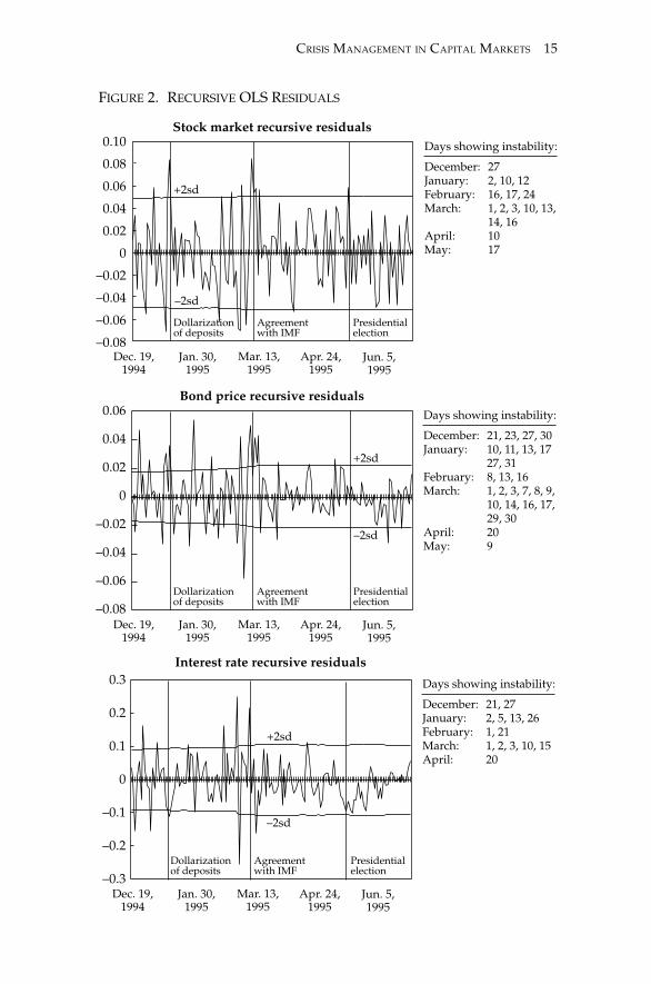
To search for the days of unexpected reaction, we computed recur-sive least squares. This methodology estimates an initial model and re-estimates the model repeatedly, using larger subsamples in everyrepetition. In each estimate a “one-step ahead” forecast was computed.The residuals were scaled such that the variance was constant.
The residuals of the different models were plotted in figure 2 for theperiod December 19, 1994, to mid-1995. Most of the residuals lie withinthe (±2 standard deviation) confidence interval, except during the peri-ods of announcements. In fact, the residuals fall outside the bands onthe days of major announcements. For instance, the residuals suggestthat the stock and bond markets rose while the interest rate decreasedon the day in which the government announced that deposits weredollarized. When news about the imminent agreement with the IMFbecame public, our estimates yield a positive reaction of the stock andbond markets, and an increase in the interest rate. The results from therecursive least squares are, in general, consistent with table 2, whichdisplays the percent change in each financial variable on the announce-ment days.7
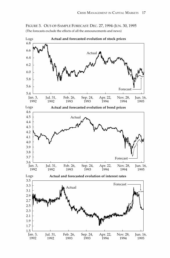
As another way to shed light on how news affected the markets, weperformed out-of-sample forecasts. To compute the forecasts, we esti-mated each of the models up to the day before any announcements weremade (December 27, 1994). Then we calculated out-of-sample forecastsfor the following six-month period. The purpose of these forecasts is toshow how the variables would have behaved if the markets had notreceived any announcements or news (namely, if the government hadremained inactive after the crisis).
The out-of-sample forecasts are plotted in figure 3. The graphs dis-play the actual and forecasted values of the stock market index, Bradybonds, and interest rate. The plots show that the actual values outper-form the forecasted ones. In other words, once the crisis had started, thecapital markets would have performed much worse if the governmenthad not taken an active role. The stock market and the bond markets
7. During March 1 and 2 the residuals for the stock and bond models fallbelow the lower band, whereas the residuals for the interest rate models lieabove the upper band. On March 3, the reverse happens. This last exampleshows that not all changes in the residuals can be clearly identified with par-ticular announcements. During those days, the debate about the future of theconvertibility plan intensified in the media, but no particular news was released.
Feb. 3, 1995: Rediscounts were limited. 1.49 –0.80 –0.34Feb. 27, 1995: The central bank charter was
modified. –0.47 –5.24 6.69Feb. 28, 1995: Reserve requirements were
increased. –0.47 –1.26 –0.61Mar. 10, 1995: An agreement with the IMF was
announced. 9.30 12.83 32.82Mar. 28, 1995: A fiduciary fund was created. 0.48 1.53 –3.63Apr. 12, 1995: A deposit insurance scheme was
established. 0.23 0.77 0.52May 15, 1995: President Menem was reelected. 2.43 1.81 –3.39
Average Dec. 20, 1994 to May 12, 1995 2.44 3.21 7.29Jul. 26, 1996: Finance minister was replaced. –0.57 –4.10 –1.63
Average Apr. 25, 1996 to Jul. 25, 1996 0.62 1.07 2.11
would not have recovered as they did, and the interest rate would haveremained higher.
To sum up, figure 2 and table 2 suggest that the dollarization of de-posits and the agreement with the IMF, among other announcements,had a positive impact on capital markets. Figure 3 suggests that theannouncements jointly had a very positive effect on the capital mar-kets. The rest of the article measures the short-run and long-run effectsof each policy announcement and news event.
Measuring the Impact of Each Announcement and News Report
To measure the short-run and long-run effects on capital markets, weconstructed two dummy variables for each announcement and newsevent. We read all major Argentine newspapers to determine the daysin which the markets received new information. The dummy variablestake the values 0 or 1. The short-run dummy variable is defined as fol-lows: Dsr
k, a= 1 and Dsrk, a +1 = 1, where a is the day the announcement was
released, while k defines the announcement. The short run includes both
CRISIS MANAGEMENT IN CAPITAL MARKETS 17
FIGURE 3. OUT-OF-SAMPLE FORECAST: DEC. 27, 1994–JUN. 30, 1995(The forecasts exclude the effects of all the announcements and news)
Logs6.8
6.6
6.4
6.2
6.0
5.8
5.6
5.4Jan. 3,1992
Actual and forecasted evolution of stock prices
Jul. 31,1992
Feb. 26,1993
Sep. 24,1993
Apr. 22,1994
Nov. 28,1994
Jun. 16,1995
Logs4.64.54.44.34.24.14.03.93.83.73.6
Actual and forecasted evolution of bond prices
3.53.33.12.92.72.52.32.11.91.71.5
Actual and forecasted evolution of interest ratesLogs
Actual
Forecast
Actual
Forecast
ActualForecast
Jan. 3,1992
Jul. 31,1992
Feb. 26,1993
Sep. 24,1993
Apr. 22,1994
Nov. 28,1994
Jun. 16,1995
Jan. 3,1992
Jul. 31,1992
Feb. 26,1993
Sep. 24,1993
Apr. 22,1994
Nov. 28,1994
Jun. 16,1995
18 Eduardo J. J. Ganapolsky and Sergio L. Schmukler
the day of, and the day after, the announcement, to account for the mo-ment the news appeared in the printed press and because some an-nouncements were made after the markets closed. The long-run dummyvariable is defined as Dlr
k, t = 1 for all t ≥ a.8
Some exceptions were made in the definition of the dummy vari-ables. The variable deposit guarantee was equal to 1 during the periodMarch 19 to April 13. At that time, the press was reporting on both thecreation of a fiduciary fund and the establishment of a deposit insur-ance scheme. It would have been difficult to disentangle the two ef-fects, so we included both of them in the deposit guarantee variable. Inthe case of reserve requirements, we used the actual requirement levelinstead of a dummy variable. We included two quantitative (rather thanqualitative) variables—reserve requirements and cash in banks—tomeasure changes in the reserve requirement policy.
The models we estimated are the following:
∆Yt = α + Φ'Dt+ Argentina Σ
L1
l = 1γ1l ∆Yt – 1
Argentina+ΣF1
f = 1γ2j ∆Zf, t – jΣ
L2
j = 0+ Σ
F2
f = 1κfj ∆Xf, t – jΣ
L3
j = 1+ εt.
As mentioned before, YtArgentina
stands for the three Argentine financialvariables we study.
In all the regressions, our interest focuses on the estimates of Φ. Theseestimates are the coefficient of Dsr
kt and Dlrkt, which stand for the short-
run and long-run effect of announcements and news, and for the im-pact of different reserve requirement levels. When φk is statistically differentfrom 0, we interpret the corresponding announcement and news to havea significant impact in explaining the dependent variable.
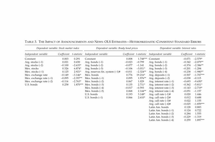
Table 3 displays the estimation results, with heteroskedastic consis-tent standard errors. The lags that repeatedly appeared to be statisti-cally insignificant across specifications have been excluded. The reportedresults are robust to many specifications, except when noted. The re-sults for each model can be summarized as follows.
(1) Stock market index: Three dummy variables were always signifi-cant and positive. The agreement with the IMF was statistically signifi-cant both in the short run and in the long run. The size of the coefficientswas also large relative to the other variables. The short-run effect of the
8. Since our specifications calculated the impact on the returns of the vari-ables, a short-term effect implies a long-term shift on the level of the variables.
CRISIS MANAGEMENT IN CAPITAL MARKETS 19
agreement had an estimated impact of around 7 percent. The dollar-ization of deposits was the third variable that always appeared signifi-cant in the short-run behavior of the stock market index. On the otherhand, the rediscount policy and the reform of the central bank charterhad negative effects on stock market prices. These last two policy mea-sures, which implied more discretionary power to the central bank (re-laxing the rules imposed by the currency board), were followed by anegative market reaction.
Among the other exogenous variables, we found that the Mexicanstock market index was highly correlated with the Argentine stock mar-ket index. The Mexican exchange rate also affected the Argentine stockmarket index. A devaluation in Mexico had a negative effect on Argen-tine stocks. U.S. bond prices were significant and positively correlatedwith the stock market index.
(2) Brady bond prices: The three dummy variables that were statisti-cally significant and positive in the stock market equation had the sameeffect on bond prices. In other words, the agreement with the IMF had apositive short-run and long-run impact on bond prices, and thedollarization of deposits had a positive short-run effect.
Other announcements and news also turned out to be significant inthe equation for bond prices. Lower reserve requirements positivelyaffected bond prices. The finance ministry had predicted that lower re-serves would have a stimulating effect on the economy—the bond mar-ket appears to have immediately reacted to that prediction. The depositguarantee and the fiduciary fund for bank capitalization had a nega-tive effect on bond prices, although this effect disappeared under somespecifications. This announcement implied a new contingent debt forthe government. The rediscount policy positively affected bond pricesin the short run. Lastly, the presidential election had a mild positiveshort-run effect on bond prices under a number of specifications. Thechange of finance minister had a negative short-term effect on bondprices.
Among the exogenous variables, Mexican Brady bond prices werepositively correlated with the Argentine ones. U.S. bond prices and liq-uid reserves of the financial system were also significantly related tochanges in Argentine bond prices.
(3) Interest rate: Some announcements and news were consistentlysignificant across the interest rate regressions. Among them, reserverequirements were statistically significant. The estimations showed thatthe greater the cash that banks are able to use, the lower the interestrate. The dollarization of deposits also lowered the peso interest rate in
TABLE 3. THE IMPACT OF ANNOUNCEMENTS AND NEWS: OLS ESTIMATES—HETEROSKEDASTIC-CONSISTENT STANDARD ERRORS
Dependent variable: Stock market index Dependent variable: Brady bond prices Dependent variable: Interest rates
Reserve requirements –0.000 –0.377 Reserve requirements –0.000 –1.759*** Reserve requirements 0.001 0.775Cash in banks 0.000 0.041 Cash in banks 0.000 0.593 Cash in banks –0.001 –2.094**Dollarization 0.003 0.657 Dollarization –0.003 –0.543 Dollarization 0.008 0.494Dollarization SR 0.045 7.758* Dollarization SR 0.023 3.384* Dollarization SR –0.118 –6.791*Rediscounts –0.013 –1.399 Rediscounts –0.003 –0.505 Rediscounts –0.011 –0.557Rediscounts SR –0.015 –1.932*** Rediscounts SR 0.011 2.522** Rediscounts SR 0.029 1.675****Central bank charter –0.004 –0.345 Central bank charter –0.003 –0.414 Central bank charter 0.038 1.267Central bank charter SR –0.030 –3.589* Central bank charter SR –0.010 –1.429 Central bank charter SR 0.039 1.254Agreement IMF 0.030 2.824* Agreement IMF 0.022 2.252** Agreement IMF –0.039 –0.981Agreement IMF SR 0.067 7.541* Agreement IMF SR 0.020 2.159** Agreement IMF SR 0.115 2.302**Deposits guarantee –0.011 –1.359 Deposits guarantee –0.018 –2.298** Deposits guarantee 0.032 1.865****Deposits guarantee SR –0.008 –1.293 Deposits guarantee SR –0.003 –0.717 Deposits guarantee SR 0.006 0.568President re-election –0.006 –1.006 President re-election –0.002 –0.602 President reelection –0.014 –1.065President re-election SR –0.011 –1.547 President re-election SR 0.010 2.625* President reelection SR –0.053 –4.212*Finance minister change 0.001 0.458 Finance minister change 0.001 1.130 Finance minister change –0.002 –0.768Finance minister change SR –0.011 –1.066 Finance minister change SR –0.004 –3.050* Finance minister change SR –0.016 –2.495**
Adjusted R-squared 0.149 Adjusted R-squared 0.566 Adjusted R-squared 0.351SE of regression 0.022 SE of regression 0.009 SE of regression 0.039Log likelihood 3482 Log likelihood 4058 Log likelihood 1904F-statistic 11.50 F-statistic 58.45 F-statistic 17.01
SR: short run, *, (**), [***]: Significant at the 1, (5), [10] percent confidence level.Note: All variables are first differences, except the ones marked with (#) and the announcement variables.
22 Eduardo J. J. Ganapolsky and Sergio L. Schmukler
the short run. On the other hand, the agreement with the IMF raised theinterest rate in the short run—as if the markets perceived that the agree-ment implied a tighter monetary policy.9 However, the long-run effectwas negative (although it is only significant in some specifications). Twoother variables were sometimes significant. The reform of the centralbank charter and the deposit insurance variable seemed to raise theinterest rate, while the presidential election was negatively correlatedwith the interest rate in the short run.
We also controlled for the overnight interest rate, total deposits, andbond prices, which have the correct sign and are statistically signifi-cant. As a foreign variable, we controlled for the index of Latin Ameri-can bonds.
As mentioned before, the reported results were robust to variousspecifications. We estimated the above models using different lag struc-tures. We also estimated the contemporaneous relationship among theArgentine financial variables using two-stage least squares. Moreover,we estimated the models using seemingly unrelated regressions, sincethere was potential cross-correlation among the equations.
The Impact of Announcements and News on Volatility
In the previous sections we analyzed the impact of news on the firstmoments of the variables. However, the residuals from the previousmodels showed some clustering in volatility. There were periods inwhich volatility was low and periods where volatility was high (par-ticularly in the aftermath of the Mexican devaluation). These residualssuggest that the variance was not constant over time. Therefore, weestimated the behavior of the variance using generalized autoregressiveconditional heteroskedasticity (GARCH) models.
The models we estimated have the following specifications:
∆Yt = α + Φ'Dt + Argentina Σ
L1
l = 1γ1l ∆Yt – 1
Argentina + ΣF1
f = 1γ2j ∆Zf, t – jΣ
L2
j = 0
+ ΣF2
f = 1κfj ∆Xf, t – jΣ
L3
j = 1+ εt ,
9. Even though a strict currency board implies the inability to set monetarypolicy, the Argentine arrangement lets the central bank use bonds as part of itsreserves. Therefore, some degree exists in which to pursue monetary policy.Also, the central bank can affect reserve requirements.
CRISIS MANAGEMENT IN CAPITAL MARKETS 23
where εt is i.i.d. N(0, σ2t) and σt = ω + Ψ'Dt + Σ
L4
p = 1τ1p εt – p + τ2j σt – j .Σ
L5
j = 1
2 2 2
In each model the variance at t depends on four elements: a constantterm ω, exogenous factors given by the news variables Dt, past vari-ances σ2
t –j , and past shocks to volatility given by ε2t –p.
GARCH models had one main advantage over the models used pre-viously. These models enabled us to test whether the announcementsand news had an impact on volatility. In other words, we were able toestimate whether financial variables became more or less stable afterthe markets receive new information. By explicitly specifying the vari-ance of εt, GARCH models also yielded efficient estimates of the pa-rameters α, Φ, γ, and κ.
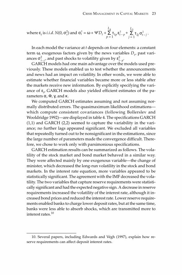
We computed GARCH estimates assuming and not assuming nor-mally distributed errors. The quasimaximum likelihood estimations—which compute consistent covariances (following Bollerslev andWooldridge 1992)—are displayed in table 4. The specifications GARCH(1,1) and GARCH (2,2) seemed to capture the variability in the vari-ance; no further lags appeared significant. We excluded all variablesthat repeatedly turned out to be nonsignificant in the estimations, sincethe large number of parameters made the convergence difficult. There-fore, we chose to work only with parsimonious specifications.
GARCH estimation results can be summarized as follows. The vola-tility of the stock market and bond market behaved in a similar way.They were affected mainly by one exogenous variable—the change ofminister, which decreased the long-run volatility in the stock and bondmarkets. In the interest rate equation, more variables appeared to bestatistically significant. The agreement with the IMF decreased the vola-tility. The two variables that capture reserve requirements were statisti-cally significant and had the expected negative sign. A decrease in reserverequirements increased the volatility of the interest rate, although it in-creased bond prices and reduced the interest rate. Lower reserve require-ments enabled banks to charge lower deposit rates, but at the same time,banks were less able to absorb shocks, which are transmitted more tointerest rates.10
10. Several papers, including Edwards and Végh (1997), explain how re-serve requirements can affect deposit interest rates.
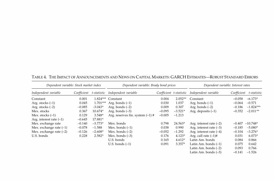
TABLE 4. THE IMPACT OF ANNOUNCEMENTS AND NEWS ON CAPITAL MARKETS: GARCH ESTIMATES—ROBUST STANDARD ERRORS
Dependent variable: Stock market index Dependent variable: Brady bond prices Dependent variable: Interest rates
Dollarization SR 0.043 3.868* Reserve requirements –0.000 –1.909** Cash in banks –0.000 –2.708*Rediscounts SR –0.033 –5.453* Dollarization SR 0.004 0.287 Dollarization SR –0.107 –4.280*Central bank charter SR –0.052 –3.404* Agreement IMF SR 0.038 2.152** President reelection SR –0.058 –2.407**Agreement IMF SR 0.077 8.486* Deposits guarantee –0.002 –1.733***
Adjusted R-squared 0.142 Adjusted R-squared 0.538 Adjusted R-squared 0.306SE of regression 0.022 SE of regression 0.009 SE of regression 0.041Log likelihood 3736 Log likelihood 4231 Log likelihood 2119F-statistic 14.18 F-statistic 73.05 F-statistic 22.80
SR: short run, *, (**), [***]: Significant at the 1, (5), [10] percent confidence level.Note: All variables are first differences, except the ones marked with (#) and the announcement variables.
26 Eduardo J. J. Ganapolsky and Sergio L. Schmukler
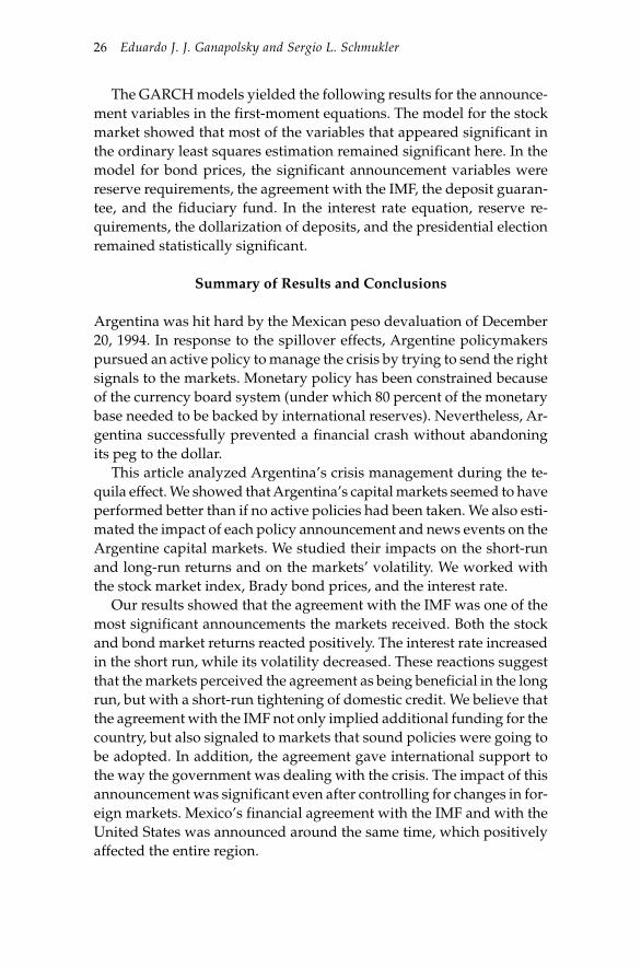
The GARCH models yielded the following results for the announce-ment variables in the first-moment equations. The model for the stockmarket showed that most of the variables that appeared significant inthe ordinary least squares estimation remained significant here. In themodel for bond prices, the significant announcement variables werereserve requirements, the agreement with the IMF, the deposit guaran-tee, and the fiduciary fund. In the interest rate equation, reserve re-quirements, the dollarization of deposits, and the presidential electionremained statistically significant.
Summary of Results and Conclusions
Argentina was hit hard by the Mexican peso devaluation of December20, 1994. In response to the spillover effects, Argentine policymakerspursued an active policy to manage the crisis by trying to send the rightsignals to the markets. Monetary policy has been constrained becauseof the currency board system (under which 80 percent of the monetarybase needed to be backed by international reserves). Nevertheless, Ar-gentina successfully prevented a financial crash without abandoningits peg to the dollar.
This article analyzed Argentina’s crisis management during the te-quila effect. We showed that Argentina’s capital markets seemed to haveperformed better than if no active policies had been taken. We also esti-mated the impact of each policy announcement and news events on theArgentine capital markets. We studied their impacts on the short-runand long-run returns and on the markets’ volatility. We worked withthe stock market index, Brady bond prices, and the interest rate.
Our results showed that the agreement with the IMF was one of themost significant announcements the markets received. Both the stockand bond market returns reacted positively. The interest rate increasedin the short run, while its volatility decreased. These reactions suggestthat the markets perceived the agreement as being beneficial in the longrun, but with a short-run tightening of domestic credit. We believe thatthe agreement with the IMF not only implied additional funding for thecountry, but also signaled to markets that sound policies were going tobe adopted. In addition, the agreement gave international support tothe way the government was dealing with the crisis. The impact of thisannouncement was significant even after controlling for changes in for-eign markets. Mexico’s financial agreement with the IMF and with theUnited States was announced around the same time, which positivelyaffected the entire region.
CRISIS MANAGEMENT IN CAPITAL MARKETS 27
Among the other announcements, the dollarization of deposits alsohad a positive effect on stock market and bond market returns. At thesame time, the dollarization decreased the interest rate. Lower reserverequirements increased bond prices (perhaps because they provided astimulus to the economy) and reduced the interest rate. However, theyseem to have increased the volatility of the interest rate.11 The fiduciaryfund for bank capitalization and the deposit insurance scheme seem tohave pushed bond prices downward and to have increased the interestrate. This increase in interest rates was partly expected, since the bank-ing sector finances the deposit insurance. The presidential election de-creased the interest rate and increased the value of Brady bonds. Whensignificant, the reform of the central bank charter had a negative effecton capital markets, increasing the interest rate and reducing the valueof stocks and bonds. The effect of the rediscount policy is ambiguous.This variable negatively affects stock prices and interest rates, while itpositively affects bond prices.
The change of minister calmed down the stock and bond markets, asestimated in the GARCH models. The markets’ nervousness about whatwas going to occur the day after Mr. Cavallo left the finance ministryappear now to have been unjustified. The stock and bond markets calmeddown when the new minister was appointed, but the short-run effecton bond prices was negative. Higher reserve requirements and the agree-ment with the IMF seemed to decrease the volatility of interest rates.
To conclude, the capital markets recovered when they received sig-nals that Argentina’s conditions had room to improve and that Argen-tina was consolidating its currency board. There was a differentiationin returns between Argentina and Mexico. The markets welcomed thesignals that demonstrated a strong commitment to the existing exchangerate peg and economic program. In this sense, the agreement with theIMF, the dollarization of deposits, and the reelection of President Menemwere welcomed by the markets. On the other hand, measures like thereform of the central bank charter—which gave more discretionarypower to the central bank—appear to have had a negative effect. It islikely that the previous government’s proposal, after the Brazilian de-valuation in 1999, to fully dollarize the economy was based on the type
11. During early 1995, there was a public discussion about the potentialcosts and benefits of lowering reserve requirements. Our estimates clearly re-flect this tradeoff.
28 Eduardo J. J. Ganapolsky and Sergio L. Schmukler
of market reactions we found in this article. The markets welcomed anymove toward dollarization.
The reaction of the Argentine capital markets stand in sharp contrastto what happened in Asia. For instance, a tightening of the monetarypolicy sent good signals to the markets in Argentina, while the reactionin Asia was mixed (as shown in Kaminsky and Schmukler 1999). More-over, Indonesia, Korea, the Philippines, Russia, and Thailand signedagreements with the IMF (for much larger amounts than $7 billion).However, the markets in these countries did not recover immediatelyafter those agreements were signed. Future research might shed lighton the circumstances in which certain policies work. For example, doesthe situation of the banking sector condition the success of a tight mon-etary policy (as discussed in Goldfajn and Gupta 1998)? Do the agree-ments with the international financial community need to be signedsimultaneously, as was the case with Argentina and Mexico? Do coun-tries need to show some commitment to confront the crisis besides call-ing on the IMF, as Argentina did? Do policymakers need to signal tomarkets that they really support the agreements?
Appendix A: Data Description
This appendix describes the series used in the paper. The data sourceswere the central bank of Argentina and Bloomberg. The listed series coverthe period January 2, 1992, to July 10, 1997, except as indicated.
We worked with the following series:
1. Stock MarketsArgentina: Merval indexBrazil: Bovespa indexChile: IPSA indexMexico: IPC indexUnited States: Dow Jones indexLatin America: We have constructed a stock market index, including
Brazil, Chile, and Mexico. The index is weighted by the relative GDP ofeach country.
2. Bond MarketsArgentina: Discount bond price indexBrazil: Discount bond price indexMexico: Discount bond price indexUnited States: U.S. Treasury price index (maturity November 2021)
CRISIS MANAGEMENT IN CAPITAL MARKETS 29
Latin America: We have constructed a bond market index, includingBrazil and Mexico. The index is weighted by the relative GDP of eachcountry.
Argentina’s bond index started on September 24, 1992; Brazil’s onJune 28, 1993; and Mexico’s and the United States’ on January 2, 1992.
3. Money MarketsArgentina: Time deposits interest rate in pesos, 30 to 59 daysMexico: Time deposits rate in pesos, 60 daysUnited States: T-bill rate in U.S. dollars, 1 monthThe Mexican data started on September 29, 1992, Argentine inter-
bank (call) interest rate on January 28, 1992, and the others on January2, 1992.
4. Argentine Financial SystemFulfillment of reserve requirements (stock) and stock of international
reserves held by the central bank. Both series ended in June 25, 1997.
5. Mexican exchange rate (pesos per U.S. dollar)
References
Baig, Taimur, and Ilan Goldfajn. 1998. “Financial Market Contagion in the AsianCrisis.” International Monetary Fund Working Paper 98/155.
Berry, Thomas, and Kith Howe. 1994. “Public Information Arrival.” The Journalof Finance XLIX (4): 1331–46.
Bollerslev, Tim, and Jeffrey M. Wooldridge. 1992. “Quasi-Maximum LikelihoodEstimation and Inference in Dynamic Models with Time Varying Covari-ances.” Econometric Reviews 11: 143–72.
Calvo, Sara, and Carmen Reinhart. 1996. “Capital Flows to Latin America: IsThere Evidence of Contagion Effects?” In Guillermo Calvo, Morris Goldstein,and Edward Hochreiter, eds., Private Capital Flows to Emerging Markets. Wash-ington, D.C.: Institute for International Economics.
Campbell, John, Andrew Lo, and A. Craig MacKinlay. 1997. The Econometrics ofFinancial Markets. Princeton, N.J.: Princeton University Press.
Ederington, Lois, and Jae Ha Lee. 1993. “How Markets Process Information:News Releases and Volatility.” The Journal of Finance XLVIII (4): 1161–91.
Edison, J. Hali. 1996. “The Reaction of Exchange Rates and Interest Rates toNews Releases.” International Finance Discussion Paper 570, Federal Re-serve Board.
Edwards, Sebastian, and Carlos Végh. 1997. “Banks and Macroeconomic Dis-turbances under Predetermined Exchange Rates.” Journal of Monetary Eco-nomics 40 (2): 239–78.
30 Eduardo J. J. Ganapolsky and Sergio L. Schmukler
Eichengreen, B., A. Rose, and C. Wyplosz. 1996. “Contagious Currency Crises.”NBER Working Paper 5681, National Bureau of Economic Research, Cam-bridge, Mass..
Elmendorf, Douglas, Mary Hirschfeld, and David Weil. 1992. “The Effect ofNews on Bond Prices: Evidence from the United Kingdom, 1900–1920.”Working Paper 4234, National Bureau of Economic Research, Cambridge,Mass.
Engel, Charles, and Jeffrey Frankel. 1984. “Why Interest Rates React to MoneyAnnouncements: An Explanation from the Foreign Exchange Market.” Jour-nal of Monetary Economics 13: 31–9.
Frankel, Jeffrey A., and Sergio L. Schmukler. 1998. “Crisis, Contagion, and Coun-try Funds: Effects on East Asia and Latin America.” In Reuven Glick, ed.,Managing Capital Flows and Exchange Rates: Lessons from the Pacific Basin. Cam-bridge, U.K.: Cambridge University Press.
Ganapolsky, Eduardo, and Sergio Schmukler. 1998. “Crisis Management in Ar-gentina during the 1994–95 Mexican Crisis.” Policy Research Working Paper1951, World Bank, Washington, D.C.
Goldfajn, Ilan, and Poonam Gupta. 1998. “Does Monetary Policy Stabilize theExchange Rate.” Working Paper, International Monetary Fund, Washing-ton, D.C.
Hardouvelis, Gikas. 1988. “Economic News, Exchange Rates and Interest Rates.”Journal of International Money and Finance 7: 23–5.
Harvey, Campbell, and Roger Huang. 1991. “Volatility in the Foreign CurrencyFutures Market.” The Review of Financial Studies 4 (3): 543–69.
Johansen, Søren. 1991. “Estimation and Hypothesis Testing of Cointegration Vec-tors in Gaussian Vector Autoregressive Models.” Econometrica 59:1551–80.
Jones, Charles, Owen Lamont, and Robin Lumsdaine. 1996. “Public Informa-tion and the Persistence of Bond Market Volatility.” Working Paper 5446,National Bureau of Economic Research, Cambridge, Mass.
Kaminsky, Graciela, and Carmen Reinhart. 2000. “On Crises, Contagion, andConfusion.” Journal of International Economics 51 (1): 145–68.
Kaminsky, Graciela, and Sergio Schmukler. 1999. “What Triggers Market Jitters?A Chronicle of the Asian Crisis.” Journal of International Money and Finance 18:537–60.
Melvin, Michael, and Xixi Yin. 1998. “Public Information Arrival, Exchange RateVolatility, and Quote Frequency.” Working Paper, Arizona State University.
Mitchell, Mark, and J. Harold Mulherin. 1994. “The Impact of Public Informa-tion on the Stock Market.” The Journal of Finance XLIX 3: 923–50.
Valdés, Rodrigo. 1996. “Emerging Markets Contagion: Evidence and Theory.”Unpublished manuscript, Massachusetts Institute of Technology.